Society of Japan
Vol. 39, No. 1, March 1996
THE MEAN-VARIANCE APPROACH TO PORTFOLIO OPTIMIZATION
SUBJECT TO TRANSACTION COSTS
Atsushi Yoshimoto
Miyazaki University
(Received April 4, 1994; Revised July 5, 1995)
Abstract Tra,nsact>ion costss are a. source of concern for port,folio managers. Due t o nonlinearity of the cost
function, the ordinary quadratic programming solution technique cannot be applied. This paper addresses the portfolio optinlization problem subject t o transaction costs. The transaction cost is assumed t o be a V-sha,ped function of difference between an existing and new portfolio. A nonlinear programming solution technique is used to solve t,he proposed problem. T h e port,folio optimiza,t,ion syst,em ca,lled POSTRAC (Portfolio Optirniza,tion System with TRAnsaction Costs) is proposed. T h e experimental analysis indicates that ignoring the transa,ction costss results in inefficient portfolios. It is also shown tlmt there does not exist statistica,lly significant difference in portfolio performance with different methods t o estimate the expected return of se~urit~ies, when considering the tra,nsact,ion costs int,o the p ~ r t ~ f o l i o return.
1. Introduction
Transaction costs are a source of concern for portfolio managers. Due to the change in expectation of a future return of securities, most a,pplications of portfolio optimization involve the revision of an existing portfolio. This revision entails both purchases and sales of securities along with transaction costs.
There are ob~erva~tions as to the ma,gnitude of the transaction costs a t the
U.
S.
stock market in literature. Schreiner and Smith [l l] estimated percentage brokerage commissions over the period from 1968 to 1978. T h e small investor had been charged more than the large investor. It was also shown that the more per share, the less commissions were. Loeb[5]
reported findings concerning the total costs, which included a ma,rket ma,ker7s spread, price concessions and commissions. The total costs of trading a given size of stock decreased with increa,se in the size of the ma,rket capitaliza,tion. For a given size of t h e ma,rket capitalization, the larger the size of trading, the more the costs were. The largest costs were associated with a large size of trading in the small market capitalization. The smallest costs were associated with small trading in the large market ~apita~lization.
In contrast, the transaction costs at the Ja,pa.nese stock market are rather fixed.
It
is a piecewise disjunctive linear function of an amount of stock to be traded. When a n amount of stock to be traded is less than1
million Japanese yen, the costs are 1.15% of its amount. Within a range of1
million to 5 million Japanese yen for trading, the costs are the sum of 2500 Japa.nese yen a,nd 0.9% of its a,mount,. From 5 million to 10 million Ja,pa,nese yen, the costs are set to 0.7% of its amount plus, 12500 Japanese yen. As can be seen, t h e costs consist of a fixed charge and a proportional charge to a,n amount of stock to be traded.A
fixed part of the costs increases up to 78500 Japanese yen as a n amount of the traded stock increases. The other part of the costs decreases down to 0.075% with increase in a n amount of the tra,ded stock.lio constructing models. It has gained widespread acceptance as a practical tool for portfolio construction. T h e problems are usually formulated with a quadratic nonlinear objective function subject to linear constraints a,nd solved by the quadratic programming solution technique. The technique simultaneously allocates securities within the portfolio construct- ing decision framework. Within the quadratic programming framework, t o avoid undesirable movement (or transaction costs) from an existing portfolio to a new portfolio, one can ap- ply turnover c ~ n s t r a ~ i n t s (Perold
[10]).
Since ~ o n s t r a ~ i n t s a,re to be formulated as a linear equation, the problem can be still solved by the quadratic programming solution technique. Introducing the turnover constraints, undesirability of having a large amount of the trans- action costs is reduced to the point a t which portfolio managers can endure. It should be noted, however, t h a t the derived portfolio from such a problem may not be t h e one that achieves an optimal tra,deoff between costs a,nd benefits. Because of a direct impact of t h e transaction costs on investment performance, a real net return of securities should b e evalu- ated by considering the costs into a,n expected return of securities. As mentioned by Arnott and Wagner [I], ignoring the transaction costs would lead to very ineffective portfolio im- plementation. Due t o the complexity of the proposed problem of searching for an optimal portfolio subject t o tra,nsaction costs, the quadratic programming solution technique cannot be utilized. This is because the transaction cost may be a separable, nonlinear, nonconvex function of a difference in holdings of new a,nd existing portfolio.The transaction costs are often incorporated into such models t h a t deal with the multi- period portfolio selection. Recent studies on the costs in portfolio optimization include Mul- vey and Vla,dimirou
[8],
Da.ntzig a,nd Infa,nger [3], a,nd Gennotte and Jung [4]. Mulvey and Vladimirou [g] modeled multiperiod financial planning problems by the stochastic network programming. Within the framework of multiscenario generalized networks, they account for the linear transaction costs by means of arc multipliers. Using multi-stage stochastic linear programs, Dantzig and Infanger [3] incorporated the transaction costs into the multi-period asset allocation problems. They solved the problem by approximating the objective func- tion by a piecewise linea,r function. Due to this linear transformation, nonlinearity of cost functions dissolved. Gennotte and Jung [4] examined the effect of proportional transaction costs on dynamic portfolio strategies for the two asset case (risky and riskless). They used a V-shaped function of a,dditional investments as proportional transaction costs, and solved the problem by mea,ns of dynamic programming.Although the transaction costs are taken into consideration by these researchers none of them has used the mean-variance approach directly using a V-shaped cost function. The objective of the paper is to address the optimal portfolio problem subject to transaction costs, and to examine the effect of the transaction costs upon portfolio performance. The proposed problem directly takes the transaction costs as a part of a portfolio return. T h e costs are assumed to be a V-sha.pe function of a new a,nd existing portfolio. Considering the tra,nsa,ction costs, the portfolio selection problem can be multiperiod. In this pa,per, however only the one-period portfolio revision is considered.
The remainder of the paper presents the portfolio problem subject to transaction costs in the next section, develops the portfolio optimization system to solve the proposed prob- lem in the third section, and provides results of comparison of portfolios with and without transaction costs in the fourth section, followed by conclusions in the last section.
2.
Portfolio Optimization Problem
A
portfolio optimization problem is often formulated with the following quadratic ex- pected utility function,E
Ut
,
where
a
is a portfolio and r_t is a security return vector and V_t is a variance-covariance matrix of security returns a t time t.A
is a given parameter.Et
[a] is a conditional expectation operand at time t. 'denotes transpose. Maximizing the expected utility is the objective of the problem,The following constraints are usually embedded,
where
1
is a unit vector. The first constraint implies that a fund is fully invested among risky and riskless securities. T h e other constraint is to prohibit short sales and borrowings. Dealing with transaction costs, the predominant strategy is to use the turnover con- straints. Letting X $ be the amount by which a proportion in the i-th security is increased,and X $ be the amount by which a proportion in the i-th security is decreased a t time t, we
ha,ve the following,
D D D D 1 I I I
where
xf
= ( z ~ ~ ~ , . T ~ z ~ , ~ ~ , , ~ z , ~ ~ ),
and 2; = (3,
x 2 1 t 1 x 3 , t 1 1 , ~ , ) ' . n is the number of securi- ties. Notice that gn is a given existing Restricting the sum of purchases or sales, the turnover constraint is formulated by,where
U
is an upper bound. Perold [10] further introduced constraints called minimum trading size constraints to reduce undesirable small trades or holdings. T h e constraint for the i-th security is disjunctive,where {li,t,l!,t} and { U ~ ~ ~ U ~ , ~ } are the admissible lower and upper region of the i-th security, X i t , at time
t .
With the turnover constraints and minimum trading size constraints, portfolio managers could avoid undesirable trading intentionally. The upper or lower limit of trades must be specified in advance by experiences. In no consideration of an effect of transaction costs on the portfolio return, however a non-optimal solution could result.In the proposed problem, the transaction cost a t time t , is assumed t o be a
V-
shaped function of a, difference between a. given existing portfolio, and a new portfolio, ~f and formulated explicitly into the portfolio return.
1 0 2 A. Yoshimoto
where c i f is a transaction cost of the i-th security a,t time
t
andki
is a constant cost per change in a proportion of the i-th security. To have the problem solved by the nonlinear programming solution technique, the absolute term on the right hand side of Equation (2.8) is further tra,nsformed into the following,(2.9) where (2.10)
(2.12)
If the difference, xit
d[t,d;t 2 0
,
Vixt,i-l, is positive (negative), d 2 ( d s ) becomes zero and d$ (d;,) becomes the difference. Due to Equation (2.1 1 ) both of d's cannot be positive at the same time. Accounting for the above transaction costs, our problem (Problem NLP) is,
Problem NLP
I I I
J ( 6 )
= m a x { a-
Et
[Q] - - \- ~t.
Vt
.
~ t } subject towhere % = ( c l t , c^,,, CS,<,
, ,
c~,,;,,)'. No additional constraints, such as turnover constraintsand minimum tra~cling size constraints, are considered. Since the transaction costs are in- corporated into the optimization framework, an optimal tradeoff between costs and benefits can be searched. It is noticeable that although the problem involves the dynamic change
in portfolio, it is only applied to two sequential periods with a given
{ x ~ , ~ - ~ } ,
not over the whole time horizon.3. Portfolio Optimization System
In
the proposed s y s t e n ~ , an expected return of each security was calculated in two ways. The first was to regard a,n arithmetical mean of the past d a t a on a security return as the expected return, while the second was to estimate the expected return by using the simple regression model with a yield spread as a n exogenous variable. Since the mean-variance asset allocation models can be highly sensitive to small perturbations in the expected return of securities and covariance, even a small cha,nge in the expected return and covariance struc- ture may lead to large variations in allocations. Using a significantly correlated exogenous variable in the simple regression model ma,y result in a far different expected return than an arithmetical mean. It is of interest to see how the transaction costs affect these variations. In what follows, each method to calculate the expected return is presented, then the proposed system is elaborated.i) Arithmetical Mean Method
Using an arithmetical mean, a return of the i-th security a t period
T,
r i ~ , is calculated from its past data,where
E&lT-l
is an arithmetical mean and calculated by,( T
- l>
to)
& i l ~ is a disturbance term,
t o
is the starting period andT
is the current period for the problem, at which a new portfolio will b e constructed. An arithmetical mean is regarded as the expected return.A va,ria,nce, vART[*], is estimated by,
A covariance for the i-th a,nd 7-th securities is given by,
( 3 . 5 )
COVT [ r i , ~,
r j , ~ ] = COVT [&i1T, c j , ~ ]and
a,n element of a varia,nce-c~varia~nce matrix,IT,
becomes:ii) Simple Regression Model
T h e second method is to use a simple regression model t o calculate t h e expected return of a security. It was assumed that a return of each security responds t o an exogenous variable with a lapse of time so tha,t the expected return of a security a t time
t
is calculated a t timet
- 1. Letting RijT-\ be an exogenous variable for the i-th security a t timeT,
the simple regression model used here is built a,s follows,104 A. Yoshimoto
where a,nd a,re unknown coefficients, and e ; , ~ is a disturbance term. T h e length of lags was set to be one period. Unknown coefficients are estimated by means of the method of least squares (see Maddala [G]).
Provided that coefficients were estima,ted, the expected return of a security is calculated by,
while a variance is estimated by Equation (3.4). An element of the resultant variance- covariance matrix is ca,lculat,ed by Equation (3.6).
iii) System Structure
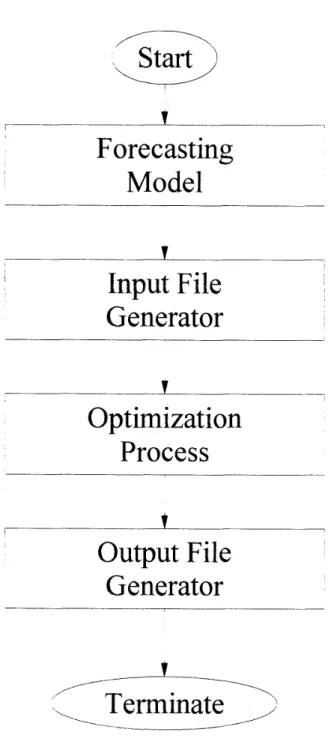
Using the above two methods to estimate the expected return of a security, the portfolio optimization system called POSTRAC (Portfolio Optimization System with TRAnsaction Costs) was proposed. The structure of POSTRAC is depicted in Figure 1. POSTRAC consists of four marin parts. The first is to calculate the expected return of each security, while the second part is the input file generator for the optimizer. T h e third part is for optimization process. Due to nonlinearity of the constraints of the problem, the quadratic programming technique was unable to be utilized. Thus, the nonlinear optimizer called GAMS/MINOS was incorporated in POSTRAC. It uses MINOS (Murtagh and Saunders 9 ) as an optimizer and GAMS (Brooke et al. [2]) as a user interface. This interface reads the input file generated in the second pa,rt. An optimal solution and other outputs from the optimizer are transformed into the output file. This is performed by the output file generator. Given the four parts, POSTRAC is built in the batch mode. It connects all four parts together in the order as in Figure 1.
4.
Model Experimentation
i )
Data DescriptionIn this section, an effect of the transaction costs on a n optimal portfolio was examined using the two methods. T h e analysis was achieved for the global asset allocation problem. Counties for investment were Japan, the U. K., the U.
S.,
Germmy, Canada, and France. In ea,ch country, two security indices, i. e., the stock ma,rket index and the Salornon Brothers bond performance index, were used. T h e data for both indices were from the database serviced by Dat astream International. The Japanese one-month CD (certificate deposit) was used as a riskless security. Its d a t a were obtained from the CAPITAL database. Foreign securities were hedged by one-month forward exchange rate, for which the Barclays Bank US dollar exchange rate quotes were used from the databaseby
Datastream International. No foreign exchange exposure was considered.A
return of each security was defined as a relative growth rate of its index value. Since the data were discrete, the following approximation was used to estimate a return,where rit is a return and
I i t
is an index value for the i-th security a t timet .
For hedged securities, a return was c a l c ~ l a ~ t e d by,where
Fit
and Silt are the forward rate and spot rate of foreign exchange for the i-th security at timet
on the basis of the Japanese currency.Forecasting
Model
,Input File
Generator
Optimization
Process
Output File
Generator
' \ \-Terminate
,
Figure
1.Structure of the proposed system POSTRAC
(Portfolio Optimization System with TRAnsaction Costs)
As for exogenous variables for security returns, a yield spread was used for the stock indices. A yield spread is defined by difference between long-term (10 years) yield-to-maturity for the bond and a reciprocal of a price-earnings ratio for the stock, so that it can b e interpreted a,s profitability of the stock relative to the bond. Since a yield spread has been said to be highly correlated to a security return a,mong portfolio managers, it is of interest to incorporate a yield spread into the model to estimate a security return, and to see its effect
1 0 6 A. Yoshimoto
on portfolio performa,nce discussed later.
A
yield sprea,d was ~ a ~ l c u l a t e d by,A
spread between long-term (10 years) and short-term( 3 months) yield-to- maturity
was used for the bond indices, since this spread can give a convenient proxy for long-term profitability of the bond. It was calculated by,Each variable is defined as follows;
YSilt : a yield spread for the i-th stock index a t time t , Spilt : a spread for the 1-th bond index a t time t ,
P E R i l t : a price-earnings ratio for t h e i-th stock index at time
t ,
L N G i t : long-term yield-to-maturity for the i-th bond index a t time t ,
SHTilt
: short-term yield-to-maturity for the i-th bond index a t timet .
A
return of each security a t timet
was regressed on the corresponding exogenous variable with the one-period la,pse of time. Monthly cla,ta from January 1985 to July 1991 were used, so that the expected return was calculated on the monthly basis. The regression period was set to24
months, resulting in the analysis period form January 1987 to June 1991.ii) Comparison of Efficient Frontiers
In
using thirteen securities, an optimal portfolio was searched.A
constant transaction cost coefficient,ki,
was a,ssumed to be 1% per cha,nge in proportion of a security. It was applied to all securities. In order to investigateif
there is a n improvement in the portfolio construction, three efficient frontiers were compared. The first one was derived by solving the following Problem NLP' in a, sequential fashion.Problem NLP' subject to I 1
E&]
-c.(
= R0 tilt =+
d 2 ),
Vi xil( - ~ i t - 1 = d^ ~ , t - dr t1t,
v i d {.
d ; = 0,
Vi d:,,~T,^Q ,
Viwhere R. is a given target return. T h e second was constructed by solving the same problem with the zero transaction costs, i. e.,
ki
=0
for a,lli.
T h e last frontier was built from the second frontier after subtracting the transaction costs from the derived portfolio return.Each frontier except the third one, was built in the following way. Firstly the upper and lower bounds of a portfolio return along the efficient frontier were searched by using the nonlinear programming technique for the first frontier and the linear programming technique for the second frontier.
A
target return, R", was increased by one-twentieth of the difference between the upper arnd lower bounds to the lower bound sequentially up to the upper bound. The number of target returns used, thus was twenty-one.A
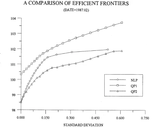
set of points specified by a return- risk (stmdard deviation) combination of an optimal solution constitutes an efficient frontier. The simple regression model wa,s used for the expected return ca,lcula,tion in this analysis. The a,nalysis period was February 1987, for which the historical data from February 1985 to January 1987 were utilized for the regression. The proportion of each security in a n existing portfolio was assigned to 7.7% (one-thirteenth). At this period, the riskless security had the least return among others.A
COMPARISON OF EFFICIENT FRONTIERS
(DATE=1987.02)98 I I I I I
l
0.000 0.150 0.300 0.450 0.600 0.750
STANDARD DEVIATION
108 A. Yashimoto
Figure 2 depicts three frontiers searched. The first frontier was labeled by NLP, the second by QP1, and the last frontier was labeled by QP2. As can be observed in Figure 2, the third frontier (QP2) wa,s inferior to the first frontier (NLP) and to the second (QP1). Since the QP2 frontier was derived after charging the transaction costs to the QP1 frontier, QP2 had less return than QP1. If an investor selects any portfolio on the Q P 1 frontier, its a,ctual position on the return-risk (standard deviation) diagram results in the QP2 frontier. Because of an effect of the transaction costs, the NLP frontier was inferior to the QP1 frontier, while it was superior to the QP2 frontier. This implies that ignoring the transaction costs results in inefficient portfolio, QP2.
Given the same level of portfolio risk (standard deviation), a difference in portfolio returns from NLP and QP2 had the largest, 0.85% per month (10.69% per year) when the risk was 0.16. In other words, incorporating the transaction costs into the optimization framework could make 0.85% more profit than would be if they were ignored. This value might vary dependent upon an existing portfolio, however inferiority of t h e QP2 frontier may remain.
iii) Comparison of Total Transaction Cost
Comparison of the efficient frontiers showed that the portfolio was improved by taking the tran~a~ction costs into account within the optimization fra,mework. In the following, a change in the tot a1 transaction costs imposed over the time horizon, was presented so that a cumulative effect of the transaction costs on portfolio performance can be revealed. For the comparison purpose, two portfolios were constructed. One was an optimal solution of the problem subject to transaction costs. This was searched by solving Problem NLP with a given lambda,
A ,
and labeled by NLP-COST in figures. T h e other was an optimal solution of the problem with the zero transaction costs. This was searched by solving the following Problem QP. The problem was set up in such a way that the objective was to maximize an expected return of a portfolio, given the same level of the risk as obtained from an optimal solution of the first problem (Problem NLP). This was labeled by QP-COST in figures. Problem Q P has a target risk constraint as well as two other constraints, Equation (4.1 1)and (4.12))
Problem
QP
subject to
where
VQ
is a given level of the risk equal to tha,t of an optimal solution from Problem NLP. Since the constraints were nonlinear, Problem Q P wa,s also solved by the same solution tech- nique, GAMSIMINOS. Comparison conducted here was to see if there exists any portfoliothat is more efficient than the derived portfolio from Problem NLP. That is, given the same level of the risk, if any portfolio has a higher return than the derived portfolio from Problem NLP, tha,t portfolio is more efficient tha,n the other. The tra,nsa,ction costs of the portfolio revision for the above Problem Q P were calculated at each period after a new portfolio was derived. Three different values for lambda,
A ,
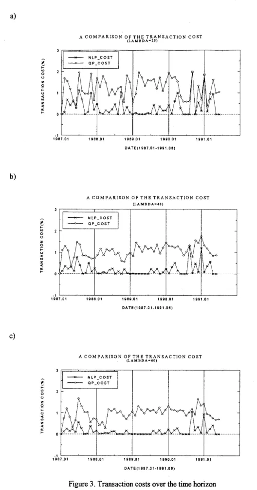
were used, 20, 40 and 60. Note that an initial portfolio a t January 1987 was derived by setting all transaction costs equal t o zero for both problems.In using the simple regression model, a change in the total transaction costs over the time horizon is depicted in Figure 3. It was observed that the less lambda,
A ,
the more the total transaction costs were for solutions from Problem QP. It is true that the less the lambda,A,
the more an investor prefers risky assets. Thus, choosing a small value for
A,
such securities that have a higher return and higher risk tend to be included into an optimal portfolio. Results in Figure 3 imply that such securities cannot keep a high level of return, resulting in the frequent revision of the portfolio. Since the transaction costs were not considered in the optimiza,tion fra,mework for Problem QP, the total transaction costs varied within a high range from 1% to 2% across all lambda's a t most periods.In
contrast, solutions from Problem NLP did not have such a tendency. T h e total transaction costs were constantly low across three values of lambda,A ,
ra,nging from 0% to 0.5%. Relatively high value above 0.5%) however, was observed during the 1987's the last 6 months of the 1990's and the first3
months of the 1991's. T h e total transaction costs of 2% mean that a new portfolio is revised completely different of the existing one.The cumulative effect of the transaction costs was as follows. T h e cumulative cost of a solution from Problem NLP became 17%
(=
1
- 0.87) forA
= 20, 10%(=
1 - 0.90) forA
= 40, 7%(=
1 - 0.93) forA
= 60 on June 1991, respectively. By contrast, for Problem QP, it was 48%(=
1 - 0.52) forA
= 20, 44%(=
1 - 0.56) forA
= 40, and 41%(=
1 - 59) forA
= 60, respectively. Comparing the two cumulative costs, a difference on June 1991 was 31% forA
= 20, it was 34% forA
= 40 and 60, which could be interpreted as a cost of ignoring the transaction costs over the time horizon.When applying the a,rithmetical mean method, one may realize that the expected return of each security did not change la,rgely over the time horizon a,s opposed to t h a t estimated by the simple regression model. Figure 4 depicts the total tra,nsaction costs in the use of the a,rithmetic,al mea,n method.
A
solution for Problem Q P resulted in a low cost ranging from 0.5% to 1.5% in most cases. This implies the less revision of the portfolio over the time horizon in comparison to the one derived by using the simple regression model. The more the value forA ,
the less the total transaction costs for solutions from Problem Q P became. A high cost was observed during the period from 1987 to 1989. For Problem NLP, the total transaction costs were almost zero over the time horizon.A
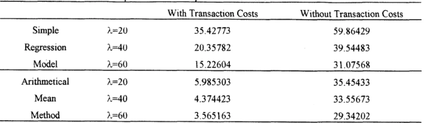
little increase in the costs was observed on November 1987, April 1990 and September 1991.The total transaction costs are directly associated with the degree of fluctuation in proportion of each security period by period. Table 1 shows the degree of fluctuation of an optimal portfolio over the time horizon. The degree of fluctuation is defined by,
where
X 2 . t : proportion of the i-th security in the portfolio a t time t
A. Yoshimoto A C O M P A R I S O N O F T H E T R A N S A C T I O N C O S T ( L A M B D A - 2 0 ) A C O M P A R I S O N O F T H E T R A N S A C T I O N C O S T ( L A M B D A - 4 0 ) 3 2 1 0 1 A C O M P A R I S O N O F T H E T R A N S A C T I O N C O S T ( L A M B D A - 6 0 )
-
N L P - C O S TFigure 3. Transaction costs over the time horizon
-
Simple regression model-
A C O M P A R I S O N O F T H E T R A N S A C T I O N C O S T ( L A M B D A - 2 0 ) A C O M P A R I S O N O F T H E T R A N S A C T I O N C O S T ( L A M B D A - 4 0 ) A C O M P A R I S O N O F T H E T R A N S A C T I O N C O S T ( L A M B D A - 6 0 )
Figure 4. Transaction costs over the time horizon
-
Arithmetical mean method-
a) X=20, b) A=40, c) A=60 3
-
a<-
N L P C O S T ÑÑ- Q P - C O S T S 2 - -A C O M P A R I S O N O F T H E P E R F O R M A N C E ( L A M B D A
-
2 0 ) 1 8 8 7 . 0 1 1 8 8 8 . 0 1 1 0 8 9 . 0 1 1 9 8 0 . 0 1 1 8 9 1 . 0 1 D A T E ( 1 8 8 7 . 0 1 - 1 9 8 1 . 0 6 ) A C O M P A R I S O N O F T H E P E R F O R M A N C E ( L A M B D A-
4 0 ) A C O M P A R I S O N O F T H E P E R F O R M A N C E ( L A M B D A-
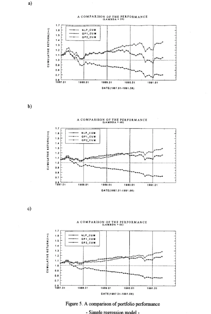
6 0 )Figure 5. A comparison of portfolio performance
-
Simple regression model-
Table 1. The fluctuation of the optimal rebalanced portfolio over the time horizon
With Transaction Costs Without Transaction Costs
Simple ?.=2U 35.42773 59.86429 Regression A=40 20.35782 39.54483 Model X=60 15.22604 3 1.07568 Arithmetical A=20 5.985303 35.45433 Mean A=40 4.374423 33.55673 Method X=60 3.565163 29.34202
This is an average Euclidian distance between the new and existing portfolio over the time horizon.
Fluctuation in solutions for Problem Q P was almost twice as much as that in solutions for Problem NLP when using the simple regression model. In contrast, using the arithmetical mean method, fluctuation in solutions for Problem Q P was about 6 to 8 times larger than that for the other. Solutions for Problem NLP yielded the smallest fluctuation. Small fluctuation was also associated with the large value of
A.
These results imply that the transaction costs play an important role in stabilizing the portfolio over the time horizon for both methods to calculate the expected return of securities.iv) Comparison of Portfolio Performance
Thus far, it was shown that the total transaction costs imposed were largely reduced once the transaction costs were taken into consideration within the optimization framework. In what follows, comparison of portfolio performance was conducted in terms of an actual return of the derived portfolio. This is because solutions from Problem NLP and Problem QP were derived under the same level of risk, so that a difference in portfolio performance is reflected in an a,ctua.l return. Under this situation, using the Sharpe measure would lead to the same results. An actual return plays a main role in judging portfolio performance. While a,n a,vera,ge return of the portfolio over the time horizon is utilized in the Sharpe measure, we used the cumulative return of the portfolio so as to investigate the effect of the transaction costs over the time horizon.
Using the simple regression model, the cumulative return of the portfolio is depicted in Figure 5. NLP-CUM represents solutions for Problem NLP, QPl-CUM is for Problem QP with the zero transaction costs, and QP2-CUM is for Problem Q P after subtracting the transaction costs. The cumula,tive return,
C&,
wa,s calculated by,where is an actua,l return vector of securities a t period
i,
so that-ii
represents an actual return of the portfolio.At the end of the a.nalysis ~ e r i o d , June 1991, NLP-CUM yielded 5%
(=
1.05 - l ) , while QP2-CUM yielded -29%(=
0.71 - 1) whenA
= 20. OnceA
was set to 40, NLP-CUM had 16%(=
1.16 - 1 ) a,nd QP2-CUM had-27%
(=
0.73 -1).
ForA
=60,
they were19%
(=
1.19 - 1) for NLP-CUM and -24%(=
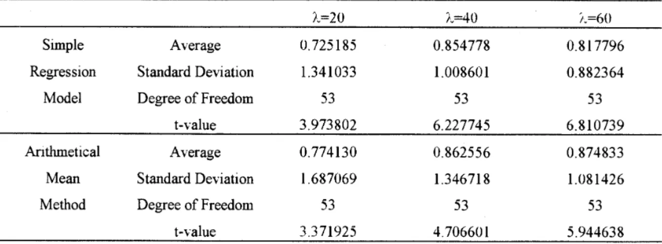
0.76 - 1) for QP2-CUM, respectively. Most likely due to the effect of the Bla,ck Monday in 1987, a downward peak was observed a t theTable 2. Results of the paired-t test: Comparison of portfolios with and without transaction costs
Simple Average 0.725 185 0.854778 0.8 1 7796
Regression Standard Deviation 1.341033 1.008601 0.882364
Model Degree of Freedom 5 3 5 3 53
t-value 3.973802 6.227745 6.810739
Arithmetical Average 0.774130 0.862556 0.874833
Mean Standard Deviation 1.687069 1.34671 8 1 .O8 1426
Method Degree of Freedom 5 3 5 3 53
t-value 3.371925 4.70660 1 5.944638
end of 1987. Large decrease in the cumulative return on August 1990 might be caused by
the eruption of the Persian Gulf War. A difference in the cumulative return of NLP-CUM
and QP2-CUM wa,s 34% for A
=20, 43% for
A
=40, and 45% for
A
=60. That is, ignoring
the transaction costs would result in about 34% to 45% reduction in the cumulative return
over 65 months, which is a,pproximately equiva,lent to 7.4% to 10.4% annual reduction.
Ignoring the transaction costs, Q P
1_CUM yielded the highest cumulative return when
A
=20, followed by A
=40 and A
=60. Once the transaction costs were subtracted from the
same portfolio, this order became opposite. QP2-CUh4 resulted in the highest value a t
A
=60, the second highest a t A
=40, and the lowest at A
=20. NLP-CUM had the same order for
the cumulative return on June 1991 as QP2-CUM. These results imply t h a t to seek the higher
expected return of the portfolio, the frequent revision of the portfolio would be necessary,
resulting in the higher transaction costs. Comparison of QP1-CUM and QP2-CUM indicated
that there exists
alarge difference in the actual cumulative return between QP1-CUM and
QP2-CUM. If one does not recognize the transaction costs, "poor" portfolio performance
may result,, a,nd its effect is a,ccumula,ted over the time horizon consta,ntly.
A change in the cumulative return in using the arithmetical mean method is delineated in
Figure 6. T h e same effect of the Black Monday on 1987 and the eruption of the Persian Gulf
War as in Figure 5 wa,s observed. For NLP-CUM, the cumulative return
011June 1991 yielded
the highest 11%
(=
1.11
- 1)a t
A
=60. The second highest 9%
(=
1.09
-1) was observed
at
A
=40, then the lowest 1%
(=
1.01
-1) a t A
=20. On the other hand, QP2-CUM had
the highest -31%
(=
0.69
-1) a,t A
=60, the second highest -32%
(=
0.68
- 1)a t
A
=40,
and the lowest -44%
(=
0.66
- 1)a t A
=20. A difference among the values was almost the
same for both cases as in Figure 5, meaning that the effect of
A
was almost the same for the
arithmetical mean method and the single regression model.
Table 2 shows results of the p i r e d t-test conducted so as t o compare performance of
NLP-CUM and QP2-CUM in terms of an actual return. A11 actual return reflects
acost
of revising t h e portfolio as well as a return from each security
initself. Using the simple
regression model, the t-value was 3.99, 6.22 and 6.81 for
A
=20, 40 and 60, respectively.
This indica,tes statistically significant superiority of NLP-CUM over QP2-CUM. This can be
also said as to the use of the a,rithmetica,l mean method. At
A
=20, the t-value was 3.37,at
A
=40, it was 4.71 and the t - d u e was 5.94 at
A
=60. Ignoring the transaction costs, one
would choose an inefficient portfolio with
ahigh probability.
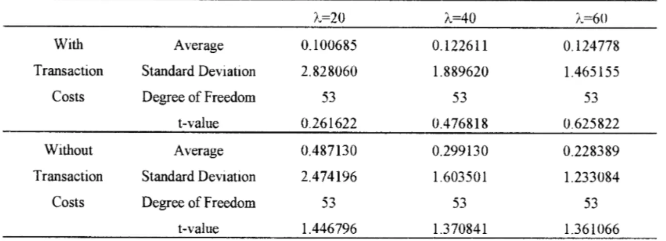
Table 3 presents results of the paired t-test to compare the actua,l return in both ways
to calculake the expected return of securities. Results showed tha,t there did not exist
aA C O M P A R I S O N O F T H E P E R F O R M A N C E ( L A M B D A 2 0 ) A C O M P A R I S O N O F T H E P E R F O R M A N C E ( L A M B D A 4 0 ) A C O M P A R I S O N O F T H E P E R F O R M A N C E ( L A M B D A
-
6 0 )Figure 6. A comparison of portfolio performance
-
Arithmetical mean method-
A. Yoshimoto
Table 3. Results of the paired-t test: Comparison of portfolios derived with different methods to calculate the expected return
With Average 0.100685 0.12261 1 0.124778
Transaction Standard Deviation 2.828060 1.889620 1.465155
Costs Degree of Freedom 5 3 5 3 5 3
t-value 0.261622 0.4768 18 0.625822
Without Average 0.487130 0.299130 0.228389
Transaction Standard Deviation 2.474196 1.603501 1.233084
Costs Degree of Freedom 5 3 5 3 5 3
t-value 1.446796 1.370841 1.36 1066
statistically significant difference among the two methods when the transaction costs were considered. In contra,st,, with the 10% ~ignifica~nce level, a, statistically significant difference was observed when ignoring the transaction costs. Notice, however, it turns out to be insignificant with the
5%
significance level.With the zero transa,ction costs, the derived portfolio was sensitive to a small change in the expected return of securities. However, if the transaction costs were taken into consid- eration, the derived portfolio became insensitive. This is because changing the weight of the selected securities in the optimal portfolio would produce not only an extra return, but also an extra cost, so that the portfolio revision would not be implemented unless its expected return were more than the costs. It is important to notice that a return of a security has uncertain characteristics, while the transaction costs are certain to be charged.
5. Conclusions
The objective of this paper was to address the portfolio optimization problem subject to tra,nsa,ction costs, a,nd to a,na,lyze a,n effect of t h e tra.nsaction costs on the derived portfolio. By f ~ r m u l a ~ t i n g the cost function directly into the portfolio return, more realistic problems are to be set up. The proposed problem had a nonlinea,r V-shaped cost function, so that the nonlinear programming solution technique was applied to solve the problem.
The predominant strategy to deal with the transaction costs has been to use additional constraints, such a.s turnover constraints and minimum trading size constraints. However, ignoring the transaction costs often results in a,n inefficient portfolio, although in some degree inefficiency of such a portfolio could be avoided by using those constraints. Searching for such a solution that a,chieves a,n optima,l tra,deoff between a cost of the portfolio revision and a benefit of security returns, rerna,ined unresolved.
In this paper, the portfolio optimization problem was formulated so as to search for an optimal portfolio subject to transa,ction costs. The problem was solved by using the nonlinear programming solution technique, GAMS/MINOS. An optimal solution from the proposed problem was statistically superior to the one derived without the transaction costs in terms of the actual return of the portfolio. This implies t h a t one has to consider the transaction costs in the portfolio construction. It should be recognized that a cost of the portfolio revision is charged with certainty, while a return of each security is not. This is an important part of the tradeoff between risk a,nd return.
regression model, to calculate the expected return of securities, it was concluded that there is not any statistica,lly significmt difference in portfolio performa,nce if the transaction costs are taken into consideration in the portfolio return. The transaction costs can play as a
penalty factor for the portfolio revision, so that portfolio components may not vary much over the time horizon. When portfolio managers are involved in forecasting a return of a
security, it is also of importance to consider the transaction costs in their performance in order to search for the efficient portfolio revision.
R e f e r e n c e s
[l] Arnott, R. D. and W.
H.
Wagner. 1990. The measurement and control of trading costs. Financial Analysts Journal. Nov/Dec:73-SO.[2] Brooke, A., D. I<endrick9 and A. Meeraus. 1988. GAMS: A user's guide. T h e Scientific Press. California. 289p.
[3] Dantzig? G. B. and G. Infanger. 1993. Multi-sta,ge stochastic linear programs for portfolio optimiza,tion. Annals of Opera,tions Research 4559-76.
[4] Gennotte,
G.
a,nd A. Jung. 1994. Inve~t~ment ~tra~tegies uncler Transaction costs: The finite horizon camsee Managen~ent Science. 40:385-404.[5] Loeb9 T . F. 1983. Trading cost: T h e critical link between investment information and results. Financial Analysts Journal. May/ June:39-44.
[6] Madclala,)
G. S.
1988. Introd~iction to econometrics. Ma,cmillan Publishing Co.) New York. 472p.[7] hfarkowitz,
H.
M. 1952. Portfolio selection. Journal of Finance. 7:77-91.[g]
Mulvey, J . M. andH.
Vladimirou. 1992. Stochastic network programming for financial planning problems. Management Science. 38: 1642-1664.[g] Murtagll)
B.
A. and M. Saunders. 1978. Large-scale linearly constrained optimization. hlathematical Programming. 1414 1-72.[l01 Perold, A. F. 1984. Large-scale portfolio opti~nization. Management Science. 30: 1143- 1160.
[l l] Scllreiner, J . and I<. Smith. 1980. The i ~ n p a ~ c t of Mayda,y on diversification costs. Journal of Portfolio Management. (summer). 6(4):28-36.
Atsushi Yoshimoto
Department of Agricultural $L Forest Economics Miyazaki University
1-1 Gakuen Kibanadai Nishi Miyazalci 889-21