Codebook Graph Coding of Descriptors

全文

(1)Vol.2015-MPS-104 No.2 2015/7/27. IPSJ SIG Technical Report. Codebook Graph Coding of Descriptors Tetsuya Yoshida1,a). Yuu Yamada2,b). Abstract: This paper proposes a method called Codebook Graph Coding to improve the standard orderless Bag of Features (BoF) representation of images for whole-image categorization tasks. Instead of the proximity of descriptors and features in the feature space, the proposed method utilizes the proximity of descriptors in each image when coding images as bag of features. For each image, the proposed method first constructs a graph to represent the locational relationship of descriptors in the image. Then, the connectivity relations encoded as a set of graphs are aggregated into another graph of features. Finally, this graph is used to encode the descriptors in each image as a pooled feature. Preliminary experiments are conducted to investigate the effectiveness of the proposed method and compared with other BoF methods.. 1.. Introduction. The “bag of word” representation in document analysis is recently extended to “bag of features” (BoF) representation for better whole-image categorization tasks [2], [5], [9]. After extracting local keypoints from images and representing them as descriptors (e.g., SIFT descriptors [11], [12]), the descriptors are clustered into so-called “visual words” (features) so that techniques developed in document processing can be used for whole-image categorization tasks. However, as in the bag of words representation in document analysis, the location of visual words in an image and the locational relationship between visual words are discarded in BoF representation. Since the locations of visual words in images seems more important compared with document analysis, use of locational relationship may contribute to improving the performance of whole-image categorization. Toward better whole-image categorization under the framework of BoF, this paper proposes a method called Codebook Graph Coding based on the proximity of descriptors. Instead of the proximity of descriptors and features in the feature space, the proposed method utilizes the proximity of descriptors in each image when encoding images as bag of features. For each image, the proposed method first constructs a graph to represent the locational relationship of descriptors in the image. Then, the connectivity relations in a set of graphs are aggregated into another graph of features. Finally, this graph is used to encode the descriptors in each image as a pooled feature. Experiments over scene15 and Caltech-101 datasets are conducted, and the performance of 1. 2. a) b). Graduate School of Humanities and Science, Nara Women’s University, Nara 630–8506, Japan Graduate School of Information Science and Technology, Hokkaido University, Sapporo, 060–0814, Japan [email protected] [email protected]. c 2015 Information Processing Society of Japan ⃝. our approach is investigated through the comparison with other BoF methods. Results are encouraging, and indicate that utilization of the proximity of descriptors in each image can lead to better performance.. 2.. Related Work. 2.1 Preliminaries A bold normal uppercase letter is used for a matrix, and a bold italic lowercase letter for a vector. For a matrix A, Aij stands for an element in A, and AT stands for its transposition. When a matrix A is not singular, its inverse matrix is denoted as A−1 . A vector with p ones (1, · · · , 1)T is denoted as 1p . 2.2 Bag of Features (BoF) Representation Bag of Features representation is often used in image analysis to represent a 2-dimensional image as a vector based on the frequencies of visual features [2], [5], [9]. SIFT [11], [12] and SURF [1] are often used for extracting local keypoints from images and representing them as vectors (called descriptors). Usually, extracted descriptors from images are clustered, and the centroids in the clusters are treated as “visual words” (features) in the images. The set of visual words is called a codebook. Then, codes of the descriptors are constructed based on the codebook, and each image is represented as a vector based on the frequencies of features in the image. Suppose each descriptor is represented as a p-dimensional vector, and n descriptors are extracted from an image. Let the descriptors be represented as a matrix X = [x1 , · · · , xn ] ∈ Rp×n . Also, suppose the codebook for a set of images is represented as a matrix B = [b1 , · · · , bm ] ∈ Rp×m , where each bj ∈ Rp corresponds to a feature. The standard BoF representation is based on hard vector quantization (VQ) [7] coding with respect to the codebook. 1.

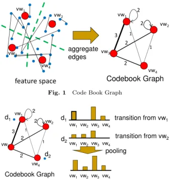
(2) Vol.2015-MPS-104 No.2 2015/7/27. IPSJ SIG Technical Report. B. Codes for the descriptors under VQ coding is determined based on the following constrained least square optimization: n ∑ C∗ = arg min ||xi − Bci ||2 C i=1. vw1. 2. (1). 2. where ci ∈ Rm is the code for descriptor xi , and || · || denotes the standard Euclidean norm. The matrix C∗ = [c1 , · · · , cn ] ∈ Rm×n denotes the corresponding codes for the descriptors X. The constraint ||ci ||ℓ0 = 1 means that there will be only one non-zero element in each code ci , which corresponds to the quantization id of xi . The nonnegative, ℓ1 constraint ||ci ||ℓ1 = 1, ci ≥ 0 means that the coding weight for each descriptor is one. In practice, the single non-zero element (quantization id) for each descriptor is usually found by the nearest neighbor search in the p-dimensional Euclidean space (which is called the feature space). After constructing the matrix C∗ , taking the row sum of C∗ (i.e., C∗ 1n ) results in an m-dimensional vector, which is the sum-pooled representation of the image under the standard BoF representation.. Codebook Graph Coding. 3.1 Descriptor Graph In our approach, the locational relationship of descriptors in an image is represented as a graph (which is called descriptor graph). Nodes in a descriptor graph corresponds to descriptors in the image, and edges are defined based on the proximity of descriptors within the image. Various proximity graphs are defined based on the proximity of nodes in the literature. Among them, Nearest Neighbor Graph (NNG) [6], Relative Neighborhood Graph (RNG) [8], and Gabriel Graph (GG) [14] are used in our approach. Locational relationship of descriptors is also used Spatial Pyramid Matching (SPM) [10] to some extent. However, since absolute locations of descriptors in the given images are used, the constructed BoF representation is not robust with respect to translation, rotation and scaling. On the other hand, since relative relations of descriptors in an image is represented as a descriptor graph, it would be robust to these transformations. Furthermore, SPM represents an approximate global geometric correspondence of descriptors, but local relationship of descriptors is represented based on their proximities in our approach. 3.2 Codebook Graph By aggregating the connectivity relations in the set of descriptor graphs, another graph called codebook graph is defined to represent the relation of features based on the locational relationship of descriptors for a set of images. Suppose descriptors are extracted from the images and clustered into m features. Hard clustering of descriptors (e.g., k-means) corresponds to defining a function f (·) from the given descriptors to the defined features. Also, suppose a set of descriptor graphs G, where each Gl (Vl , El ) ∈ G corresponds to the descriptor graph for the l-th image, is already. c 2015 Information Processing Society of Japan ⃝. aggregate vw 3 edges. vw3. 1. 2. vw4. vw4. Codebook Graph. feature space Fig. 1. d1. vw2. 1. 3. s.t.||ci ||ℓ0 = 1, ||ci ||ℓ1 = 1, ci ≥ 0, ∀i. 3.. 2. vw1. vw2. Code Book Graph. 2. vw1. 2. vw2. d1. transition from vw1 vw1 vw2 vw3 vw4. 1. 3 2. d2. 1. vw3. d2. 2. transition from vw2 vw1 vw2 vw3 vw4. pooling. vw4. Codebook Graph Fig. 2. vw1 vw2 vw3 vw4. Coding using a Code Book Graph. constructed. Here, Vl denotes the nodes, and El denotes the edges in Gl . Construction of codebook graph is illustrated in Fig. 1. In the codebook graph, each feature (visual word) is represented as a node. The edge weight between a pair of nodes vwi and vwj (with feature IDs i and j) in the codebook graph is defined as: ∑ wij = |{(vs , vt ) ∈ El |f (vs ) = i ∧ f (vt ) = j}| Gl ∈G,vs ∈Vl ,vt ∈Vl. (2) where vs and vt are vertices in Gl , and |{·}| denotes the cardinality of the set. Intuitively, weight wij in eq.(2) corresponds to the number of edges between the sub-region dominated by i-th feature vwi and the sub-region dominated by j-th feature vwj in the feature space. 3.3 Codebook Graph Coding Codes of descriptors under the proposed Codebook Graph Coding (CGC) are defined based on the transition probability in the codebook graph as well as the nearest neighbor of each descriptor. As in the standard BoF, the nearest feature for each descriptor is first determined. Then, the transition probability from the feature to all features in the codebook is used when defining the code for the descriptor. Finally, the codes of the descriptors in an image are pooled together to define the pooled feature of the image. These processes are summarized in Fig. 2. For a given image, let C0 denotes the codes of descriptors based on VQ coding in eq.(1). The edge weights defined in eq.(2) can be represented as a square matrix W ∈ Rm×m . Also, by defining the degree vector d = W1m , the degree matrix of the codebook graph is defined as a diagonal matrix D = diag(d) *1 . Then, based on the transition provability *1. Each element in d is placed on the diagonal element in D, and non-diagonal elements in D are set to zeros.. 2.

(3) Vol.2015-MPS-104 No.2 2015/7/27. IPSJ SIG Technical Report. matrix, which is defined as P = D−1 W, the codes for the descriptors by CGC are define as:. Table 1 CR. 1-NNG 0.873. Results of preliminary experiments 3-NNG 0.871. 5-NNG 0.874. RNG 0.870. GG 0.866. grid 0.818. C = PC0 = diag(W1m )−1 WC0. (3). Finally, the defined codes are pooled together to get the corresponding pooled feature of the image. The standard pooled feature in BoF is based on sum pooling [10], which is defined as c = C1n . However, since max pooling [3], which takes the maximum value for each row in C, is reported to contributes to improving the linear separability of the pooled features, max pooling is used in CGC.. 4.. Evaluation. 4.1 Experimental Setting Experiments for whole-image categorization tasks were conducted over scene15 dataset *2 and Caltech-101 dataset *3 . The former dataset contains scenery images, and the latter contains general object images. In the experiments, a specified number of images for each class (category) were selected as training data, and the remaining images were treated as test data. Since the number of images contained in each class drastically differs in these datasets, 100 images for each image were selected as test data in scene15, and 30 images were selected as test data in Caltech-101. As the quality measure of image classification, Classification Rate (CR) was used in the experiments. CR is defined as: CR =. number of correct images Number of test images. (4). SIFT descriptors [11], [12] were extracted from each image, and the extracted descriptors were clustered using kmeans to define the codebook. After encoding the descriptors in each image, the codes were normalized under ℓ2 norm. Finally, a pooled feature of each image was constructed from the codes using max pooling [3]. When classifying images with respect to the constructed pooled features, we used SVM [4], which is known with its high classification performance. Since the standard SVM is originally designed for two-class problem, we used One-vsOne Linear SVM to classify multiple classes in the datasets. One-vs-One SVM realizes multiple-class classification by conducting all the pairwise classification. However, when the number of classes is large (e.g., 101 classes in Caltech101), its takes too much time since the number of combination of classifications increases. Thus, for reducing the running time in classification, we used a simple linear kernel in SVM. As for comparison, experiments were conducted for 1) the standard BoF (as baseline), 2) Spatial Pyramid Matching (SPM) [10], 3) Locality-constrained Linear Coding(LLC) [15], and 4) Codebook Graph Coding (CGC) in Section 3. *2 *3. http://www-cvr.ai.uiuc.edu/ponce grp/data/ http://www.vision.caltech.edu/Image Datasets/Caltech101/. c 2015 Information Processing Society of Japan ⃝. Table 2. characteristics of code book graphs. mean degree average path length. 1-NNG 150.46 1.85. grid 737.19 1.27. 4.2 Preliminary Experiments The performance of our method depends on i) sampling of descriptors from images, and ii) type of proximity graph for the descriptor graphs in Section 3.1. We first report their influences in our method. As for the sampling of descriptors, two kinds of sampling, namely, a) sparse sampling, and b) dense sampling, have been widely used in the literature. Sparse sampling locates keypoints only for distinctive invariant locations in an image (as in the original SIFT algorithm [11], [12]). On the other hand, dense sampling uniformly samples keypoints from an image, irrelevant to the properties of keypoints. Usually keypoints are located over some grid in the image, and arranged in a matrix-like grid in the image. For a) sparse sampling, keypoints were located by SIFT algorithm in each image, and their SIFT descriptors were connected as a descriptor graph. Five types of proximity graphs were evaluated: Nearest Neighbor Graph (NNG) [6] (the number of neighbors were set to 1, 3, 5), Relative Neighborhood Graph (RNG) [8], and Gabriel Graph (GG) [14]. As for b) dense sampling, the width of grid was set to 5 pixels, the scale in SIFT algorithm was set to 16, and the sampled SIFT descriptors were arranged as a gid graph. The codebook size (the number of features) m was set to 1024, and 10 classes from Caltech-101 were used in the experiment. The results are summarized in Table 1. For the standard BoF representation, it is known that dense sampling or random sampling of keypoints contributes to improving the performance of classifiers, albeit the number of descriptors drastically increases [13]. On the other hand, the results in Table 1 indicate that dense sampling degrade the performance of CGC. Our current conjecture for this observation is that, when the number of edges in the codebook graph increases, the graph gets densely connected. Since the transition probabilities from nodes (features) becomes similar to each other as the connectivity of nodes increases, the codes of descriptors become almost the same with respect to a densely connected codebook graph. To verify this, the average degree and the average path length of 1-NNG (with the least number of edges) and of grid graph (with the largest number of edges) are shown in Table 2. The results in Table 2 indicate that almost all nodes are connected in grid graph. Thus, this might be the reason for the observation in Table 1. Based on the above observations, in the following experiments, we used sparse sampling for extracting descriptors, and 1-NNG for descriptor graph. 3.

(4) Vol.2015-MPS-104 No.2 2015/7/27. IPSJ SIG Technical Report. Table m base SPM LLC CGC. 3 Scene15 w.r.t. CR 1024 2048 4096 0.559 0.566 0.561 0.560 0.593 0.613 0.600 0.620 0.626 0.535 0.573 0.597. References [1]. [2] [3]. Table 4. Caltech-101 (w.r.t. CR) m BoF SPM LLC CGC. 1024 0.369 0.435 0.413 0.310. 4.3 Results The results of scene15 are summarized in Table 3. The codebook size m was set to 1024, 2048, and 4096 in the experiments. In general, class separability improves as the number of features increases. The results in Table 3 match this phenomenon. In addition, since the codebook graph gets sparsely connected as m increases, the codebook size will affect more to CGC, compared with other methods. Unfortunately, although CGC showed comparable performance, and outperformed the standard BoF, it could not outperform other methods. Since the number of classes is large in Caltech-101, in order to reduce the running time for classification, the codebook size m was set to 1024 for Caltech-101. The results are summarized in Table 4. Unfortunately, CGC could not outperform even BoF in terms of the overall classification rate. However, for some classes, the proposed method outperform LLC and SPM.. 5.. [4] [5]. [6] [7] [8] [9] [10]. [11]. [12] [13]. Concluding Remarks [14]. This paper proposed a method called Codebook Graph Coding to improve the standard orderless Bag of Features (BoF) representation of images for whole-image categorization tasks. Instead of the proximity of descriptors and features in the feature space, the proximity of descriptors in each image is used when coding images as bag of features. For each image, the proposed method first constructs a graph to represent the locational relationship of descriptors in the image. Then, the relations encoded as the graphs are aggregated into another graph of features. Finally, this graph is used to encode the descriptors in each image in BoF representation. Preliminary experiments are conducted to investigate the effectiveness of the proposed method. By using sparse sampling for extracting descriptors from images and 1-NNG for defining descriptor graphs, our method is compared with the standard BoF, SPM and LLC.. [15]. Bay, H., Tuytelaars, T. and Van Gool, L.: SURF: Speeded Up Robust Features, Proceedings of the 9th European Conference on Computer Vision, ECCV’06, Berlin, Heidelberg, Springer-Verlag, pp. 404–417 (2006). Bosch, A., Mu` noz, X. and Mart´ı, R.: Which is the best way to organize/classify images by content?, Image and Vision Computing, Vol. 25, No. 6, pp. 778–791 (2007). Boureau, Y.-L., Ponce, J. and Lecun, Y.: A Theoretical Analysis of Feature Pooling in Visual Recognition, 27TH International Conference on Machine Learning, HAIFA, ISRAEL, ICML’10 (2010). Cristianini, N. and Shawe-Taylor, J.(eds.): An Introduction to Suport Vector Machines and Other Kernel-based Learning Methods, Cambridge University Press (2000). Csurka, G., Dance, C. R., Fan, L., Willamowski, J. and Bray, C.: Visual categorization with bags of keypoints, Workshop on Statistical Learning in Computer Vision, ECCV’04, pp. 1–22 (2004). Eppstein, D., Paterson, M. and Yao, F.: On NearestNeighbor Graphs, Discrete and Computational Geometry, Vol. 17, No. 3, pp. 263–282 (1997). Gersho, A. and Gray, R. M.: Vector Quantization and Signal Compression, Springer (1991). Jaromczyk, J. and Toussaint, G.: Relative neighborhood graphs and their relatives, Proceedings of the IEEE, Vol. 80, No. 9, pp. 1502–1517 (online), DOI: 10.1109/5.163414 (1992). Jurie, F. and Triggs, B.: Creating Efficient Codebooks for Visual Recognition, Proc. of the 10th IEEE International Conference on Computer Vision, pp. 604–610 (2005). Lazebnik, S., Schmid, C. and Ponce, J.: Beyond Bags of Features: Spatial Pyramid Matching for Recognizing Natural Scene Categories, IEEE Computer Society Conference on Computer Vision and Pattern Recognition, Vol. 2, pp. 2169–2178 (online), DOI: 10.1109/CVPR.2006.68 (2006). Lowe, D. G.: Object Recognition from Local Scale-Invariant Features, Proceedings of the International Conference on Computer Vision, ICCV ’99, Vol. 2, Washington, DC, USA, IEEE Computer Society, pp. 1150–1157 (online), available from ⟨http://dl.acm.org/citation.cfm?id=850924.851523⟩ (1999). Lowe, D. G.: Distinctive image features from scaleinvariant keypoints, International Journal of Computer Vision, Vol. 60, No. 2, pp. 91–110 (2004). Nowak, E., Jurie, F. and Triggs, B.: Sampling Strategies for Bag-of-Features Image Classification, 9th European Conference on Computer Vision, ECCV’06, Springer, pp. 490–503 (2006). Ruben., G. K. and R, S. R.: A new statistical approach to geographic variation analysis, Systematic Zoology, Vol. 18, pp. 259–278 (online), DOI: 10.2307/2412323 (1969). Wang, J., Yang, J., Yu, K., Lv, F., Huang, T. and Gong, Y.: Locality-constrained Linear Coding for image classification, IEEE Computer Society Conference on Computer Vision and Pattern Recognition, CVPR’10, IEEE, pp. 3360– 3367 (online), DOI: 10.1109/CVPR.2010.5540018 (2010).. Acknowledgment This work is partially supported by the grant-in-aid for scientific research (No. 24300049) funded by MEXT in Japan.. c 2015 Information Processing Society of Japan ⃝. 4.

(5)