Title
Zhenyu Gao
A Thesis in the Field of Civil Engineering for the degree of Doctor of Philosophy
Kagawa University September 2018
Analysis on urban development using spatial modelling
technique under data constraints in China
Analysis on urban development using spatial modelling
technique under data constraints in China
Abstract
Today, more than 50% of the global population resides in urban environments and urban population will add another 2.5 billion people by 2050, with the most part of the increase concentrated in developing countries. To meet the needs of this rapid urbanization, demand for urban built-up areas and rail transit systems all around the world have grown. The impacts of such urban developments need to be elaborated for an effective management of urban system, even with the biggest challenge that most of the spatially-resolved statistical data are in unavailable condition.
The purpose of this thesis is to develop models that incorporate remote sensing data and open data with neo-classical urban economic model and graph theory to evaluate two types of urban development under data limitation. One is the evaluation of 3 Chinese cities’ urban sprawl from a region-wide perspective, and the other is the evaluation of Beijing’s rail transit network from a network topology perspective.
They notably account for how urban development affect location choice of city dwellers and economic entities. The proposed monocentric urban economic model adds a building developer to separate land and housing markets in analyzing housing consumption. It models the tradeoffs between accessibility and land rents in housing markets in a monocentric urban formulation. Thus average traffic and residential cost can be figured out according to the interactions among three agents, household, developer, and landowner. The centrality-based model determines the concentration of economic activities, which is an integration of a centrality-based index that identities the importance of a location affected by
urban rail transit network shape, and potential accessibility that represents the ease of reaching to economic activity. The results of two applications are compared with some available statistical data and connection between the two models are discussed for future development.
Overall, two proposed models developed by the means of spatial modelling technique show their applicability, validity and possibility as a quick evaluation tool for urban planning under data constraints. The methods presented here can particularly be useful to urban/rail transit planners on the issues of urban transformation with efficient management. Spatial modelling technique involving open spatial data is confident of widespread use in urban spatial analysis in the future.
Table of Contents
Abstract ... ii
List of Tables ... vi
List of Figures ... vii
Chapter 1. Introduction & contribution ... 1
1.1 Introduction ... 1
1.2 Urbanization and URT network. ... 4
1.3 Contribution ... 5
Chapter 2. Literature review ... 10
2.1 The evolution of urban spatial structures. ... 10
2.2 Urban Development Intensity (UDI) ... 13
2.3 Urban model ... 15
2.4 Centrality ... 18
2.5 Accessibility ... 20
Chapter 3. Application I: a monocentric urban economic model ... 23
3.1 Methodology ... 23
3.1.1Monocentric urban economic model ... 24
3.1.2Definition of “urban area” ... 28
3.2 Data ... 29
3.2.1Data collection and parameter estimation” ... 29
3.2.2 Extracting intra-urban areas... 33
3.3 Results and analysis ... 33
3.3.1Variation in urban area and population ... 33
3.3.2 Variation in traffic and residential conditions ... 34
3.3.3 Discussion of the monocentric urban economic model ... 38
3.4 Summary ... 39
4.1 Methodology ... 43
4.1.1Centrality measures ... 44
4.1.2 Centrality-based index of a Location (CL) ... 45
4.1.3 Potential Accessibility (PA) ... 46
4.2 Data source ... 47
4.2.1Beijing URT condition ... 47
4.2.2Nighttime light VIIRS DNB ... 48
4.2.3Distribution of commercial facilities ... 49
4.3 Results and analysis ... 50
4.4 Summary ... 55
Chapter 5. Exploration of two models for future direction ... 57
5.1 Polycentric city ... 57
5.2 One possibility of future directions by integrating two perspectives. ... 60
Chapter 6. Conclusion and future direction ... 62
References ... 65
Appendix A. Monocentric urban economic model ... 73
1. Households ... 73
2. Developers ... 75
3. Equilibrium state ... 76
List of Tables
Table 1. Collected data. ... 30
Table 2. Estimated parameters (p-values are given within parentheses). ... 30
Table 3. Citywide average population density and growth coefficients... 34
Table 4. Statistical data and estimated results. ... 35
List of Figures
Figure 1. Estimated urban growth per hour through a combination of natural internal
growth and migration in selected world cities. ... 1
Figure 2. The development of BRT, LRT and Metro since 1981. ... 2
Figure 3. The development of urban rail transit in China over the past three decades. ... 2
Figure 4. The relation between population increase and sub-center generation. ... 4
Figure 5. Attentions of urban itself and URT. ... 6
Figure 6. An overall perspective from urban sprawl. ... 6
Figure 7. A perspective from URT network shape. ... 7
Figure 8. Definition of Urban Terms. ... 11
Figure 9. Subdivision of urban areas in Toronto. ... 14
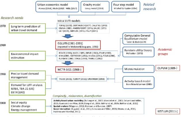
Figure 10. Summary of evolution of LUTI models. ... 17
Figure 11. Applications of network centrality over time... 19
Figure 12. Generic accessibility indicators... 21
Figure 13. Analytical flow. ... 24
Figure 14. The way to fit a real-life city of an irregular shape into the mechanism of monocentric urban model. ... 25
Figure 15. Schematic diagram of the bid-rent-based urban model. ... 26
Figure 16. Definition of urban boundary. ... 27
Figure 17. Beijing intra-urban area in 2003 (left) and in 2013 (right). ... 32
Figure 18. Nanjing intra-urban area in 2003 (left) and in 2013 (right). ... 32
Figure 19. Haikou intra-urban area in 2003 (left) 2013 (right). ... 33
Figure 20. Simulated results of composite goods consumption, floor rent and floor area consumption per capita. ... 36
Figure 21. Simulated results of commuting cost, utility and disposable time per capita. . 36
Figure 22. Urban evolution from monocentric to polycentric URT development. ... 43
Figure 23. Analytical flowchart. ... 44
Figure 24. Illustration of the concept CL (Centrality-based index of a Location). ... 46
Figure 25. Illustration of the concept PA (Potential Accessibility). ... 47
Figure 26. Beijing URT in 2015 ... 48
Figure 27. VIIRS DNB data in study area. ... 49
Figure 28. Kernel density of commercial facilities. ... 50
Figure 30. Result of potential accessibility. ... 51
Figure 32. Correlation between integrated values and kernel density of facilities ... 53
Figure 33. Extraction of urban area with top 1% values of the integrated indicator. ... 53
Figure 34. Extraction of urban area with top 2.25% values of the integrated indicator. ... 54
Figure 35. Extraction of urban area with top 4% values of the integrated indicator. ... 54
Figure 36. No clear-cut definition for identification of polycentric urban structure. ... 58
Figure 37. Relationship between two perspectives of investigating urban development .. 59
Chapter 1.
Introduction & contribution
1.1 Introduction
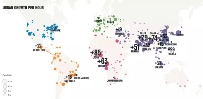
Urban population as a proportion of total population has risen from 47% in 2000 to 54% in 2014. More than 90% of this growth has come from developing countries and this trend is likely to continue over the next few decades. Today, the fraction of the global population residing in urban environments is nearly 50% and is projected to rise to 70% by 2030 (United Nations 2013). In 2030, there will be nearly 5 billion people in Asia alone, more than triple that of North America, Latin America and Europe combined, which can be inferred from the rapid rate of urban growth as shown in Fig. 1.
Source: https://www.theguardian.com/cities/2015/nov/23/cities-in-numbers-how-patterns-of-urban-growth-change-the-world
Figure 1. Estimated urban growth per hour through a combination of natural internal growth and migration in selected world cities.
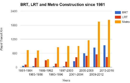
Source: https://www.itdp.org/2017/02/17/rapid-transit-trends/
Figure 2. The development of BRT, LRT and Metro since 1981.
Fig. 2 illustrates that along with rapid urbanization, besides urban built-up area, traffic network systems have grown rapidly all the globe, especially urban rail transit (URT) network. An indicator normalized kilometers built by population, Rapid Transit to Resident Ratio (RTR), which compares the length of rapid transit lines (including rail, metro, and BRT) in kilometers in each country with its urban population, has quickly risen over the past decade. In the eye of city dwellers, the higher the RTR is, the coverage of accessible URT is larger. In China, the rapid rise in RTR is thanks mostly to a boom in Metro and BRT investments (Fig. 3).
The correspondingly impacts brought by the changes in urban spatial morphology (Jiao, L 2015) as well as URT network system (Salvati and Carlucci 2014, Kai, L. et al., 2016, Gonzalez-Navarro & Turner 2016) deserve careful study for an effective management of urban system, as do the key factors affecting location choice of urban residents and economic entities. When it comes to carry out studies on such topics, one of the biggest challenges in developing countries is that most of spatially-resolved statistical data are unavailable in most case. Conventional ways of data acquisition for urban models in urban analysis are manual work, which consumes huge amounts of manpower and time to get direct information. Besides, the reliability of information is heavily influenced by different statistical methods and frequencies. Using automatically collected sensor data may not give direct information, but with the analysis and modeling method, required information can be extracted from it.
Therefore, one reachable strategy is to adopt a spatial modelling technique to develop models that incorporate remote sensing data and open data under data limitation.
1.2 Urbanization and URT network.
This rapid urbanization accelerates the migration of population into urban areas (United Nations 2016) and the development of URT network all around the globe. The emergence of mega-cities brings new challenges for the management of urban land-use and transportation system. More infrastructure is required to provide essential services not only because of the needs of living but also the needs of global competition. Meanwhile, these countries are also experiencing environmental issues, which damages city dwellers’ quality of life.
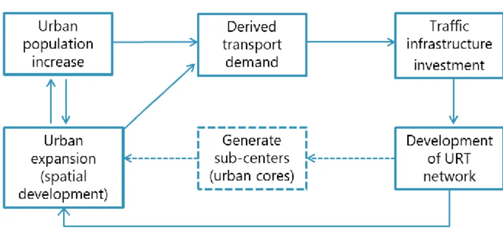
Dash line represents the process that does not necessarily happen
Figure 4. The relation between population increase and sub-center generation.
Therefore, how to effectively manage urban system to let people move smoothly and live comfortably is critical for policy makers. Nonetheless, cities evolve constantly and it is not easy to handle all its aspects that include land-use, traffic, water, energy, finance and many more. It is definitely a positive effect on sustainable development if we have more evidences to see how urban region has changed from the overall perspective, or look deeper into details of locations from intra-urban perspective.
In particular, for this thesis, the overall perspective stands for how the average traffic and residential cost change along with urban expansion. Then, given a specific urban, the importance and convenience of a location is assessed from intra-urban perspective focused on URT network shape. URT system provides sustainable mobility via an interconnected network that significantly influences livability, economic activity, urban transformation and social development. Large-scale constructions of URT stations are underway across populous cities in developing countries, aiming to resolve traffic congestion because of the rapid urbanization and motorization. Urban spatial morphology and the shape of URT network interact closely showed in Fig. 4. Urban spatial morphology determines the shape of URT network at first. Then urban extent is likely to be in accordance with URT network, as URT network provides great benefit for commuters (city dwellers) and economic entities. Locations relative to URT network have played an important role in affecting location choice. Additionally, a location relative to stations is becoming highly valued by developer as one of its core developing strategies. The exploration of integrating two perspectives mentioned above will offer more practicable advices for a sustainable urban development adapt for the future.
1.3 Contribution
Urban planning is a complicated process that balances the considerations from many different fields. Fig. 5 shows that given an urban area, what is the equilibrium state of urban development economically, and then investigating how much economic activities are related to public traffic network. Public traffic network, especially URT network, is expected to improve the condition of mobility and congestion, so acquiring an understanding of the relationship between URT and local economic concentration will be beneficial for
arrangement of urban layout. The main target of this thesis is to develop models to estimate urban development in developing countries in the context of data limitation from two perspectives illustrated in Fig. 6 (an overall perspective from urban sprawl) and Fig. 7 (an intra-urban perspective from URT network shape), and further to integrate these models towards a way of expanding the proposed model with more flexibility even in cased of evaluation of polycentric urban development.
Figure 5. Attentions of urban itself and URT.
Figure 7. A perspective from URT network shape.
More specifically, urban models adapt for current urban system have become more complex, which is challenging for data collection that required by models. Various extensions of the c model have been studied to date; however, most of this research remains qualitative, and gaps remain between theoretical and empirical findings. Furthermore, empirically multi-regional/national quantitative simulations are few but highly expected. This is not only because of the shortage of spatially- disaggregated data, but also the computational efficiency/cost. Spatial modelling technique emphasizes the role of space and models the patterns of city dwellers’ spatial behavior to understand the processes of urban development, showing practicability and validity as a quick evaluation tool for urban planning.
In the view of urban system itself, this thesis seeks first to expand the classical urban model to make it applicable to large-scale simulation by involving in open satellite data in developing countries today, whose features include massive urbanization, population growth, building construction, and urban expansion. Also this thesis introduces a market for residential floor space and developers who provide this space. A dataset is prepared for building an extended bit-rent model that includes socioeconomic and spatial data derived from remote-sensing satellite data. A comparison between observed and simulated results in
three Chinese cities is conducted to examine the applicability of the extended model, and to filter the key indices as well.
In the view of URT network shape, actual spatial distance is incorporated into topological centrality properties of URT network aiming to amplify its impact in real-life space. An index reflected the importance of a location affected by URT network shape was proposed based on centrality. Potential accessibility is defined as the ease to economic activities, and local attractiveness of economic activities is determined by the values of nightlight time data. Integration of centrality-based index and potential accessibility offers a new investigation way to explore the concentration of economic activities from the viewpoint of URT shape if a suitable benchmark is given. A case study is carried out in Beijing, the result of which is validated in comparison with the observed distribution of commercial facility points.
The fundamental issues behind this work is inaccessible spatial-detailed data in developing countries. Can we overcome data constrains with success in large-scale simulation? This thesis provides some practical experience regarding this question. Additionally, it should be mentioned that although large-scale simulation is possible, there are shortcomings in this work, which will be introduced in later chapters.
The remainder of this thesis is organized as follows.
Chapter 2 reviews related literature, with respect to the evolution of urban structure, urban development intensity, urban model, centrality, and accessibility. Chapter 3 develops the classical urban model and applies the developed monocentric urban economic model to three Chinese cities from an overall perspective of urban sprawl. Chapter 4 presents a specific case of Beijing URT network to integrate a centrality-based index with potential accessibility
to test the concentration of economic activities from a perspective of URT network shape. Chapter 5 explores more about two proposed methods for future direction. Finally, chapter 6 offers a brief conclusion.
Chapter 2. Literature review
Over the past decades, a form of strong but heterogeneous sprawl has happened in many urban areas because of global urbanization. This global trend toward urbanization is expected to be particularly prominent in developing countries, where urban infrastructure is typically far from adequate. Our concern are therefore arise regarding the process of urban changes and its impacts, which need to be elaborated for an effective management of urban system, even most of the spatially-resolved statistical data are in unavailable condition. In some cases, as a result of well-developed urban traffic network, polycentric spatial structure has shown up in some contemporary cities as a result of the urban transformation of decentralization. Therefore, besides monocentric urban development, polycentric urban development is also essential for us to understand.
In this section, the emergence of such spatial structure, as well as theories and methods that are closely related to measure such spatial structure under data limitation, are reviewed.
2.1 The evolution of urban spatial structures.
Cities have complex shapes and great complexity in their internal structure which seems hard to obtain consensus for classification. In a certain way every city is unique, and generally, monocentric and polycentric urban spatial structures are two main types that emerges during the process of urban evolution. Fig. 8 below illustrates some definition of urban terms and the relationship between metropolitan areas and their component parts.
Source: Demographia World Urban Areas, http://demographia.com/db-define.pdf Figure 8. Definition of Urban Terms.
The physical city (urban area) means the physical expanse, or area of continuously built-up urbanization, which is simply the extension of urbanization. The functional City (metropolitan area) means the functional expanse, which is also the economic expanse. The metropolitan area includes the built-up urban area and the economically connected territory to the outside. Parts of the urban administration area outside the core are considered as suburbs.
Daniel Arribas-Bel & Fernando Sanz-Gracia (2014) point out that urban economics and urban geography have long been shaped by theoretical and empirical debates over monocentric city and polycentric city, regarding the internal structure of metropolitan regions and the number of centers with high employment density.
The monocentric urban structure portrays a city with a fixed population and within which city dwellers with a given income level living around a central business district (CBD). Each city dweller travels to CBD for work. Since commuting is costly and increases with distance from the CBD, individual differences into consideration determines living locations close or far to the city, so the rent price and density of housing adjust to clear the market. In particular, land for housing/business becomes more expensive closer to the CBD, which prompts developers to economize on the use of land by building more dwellings per unit of land. The city structure is characterized by a higher density with taller buildings close to the CBD and a lower density with lower building heights on the fringe.
As the morphology and function of cities have evolved so fast over the past decades, recent theoretical and empirical researches in urban economics have pay more attentions on polycentric urban structure, which has multiple employment centers (sub-centers). Sub-centers (Josep Roca Cladera et al., 2009) appear varying degrees of influence on urban spatial patterns. Empirical evidences demonstrate that some urban areas are experiencing transformation to polycentric urban structure with the clustering of economic activities in sub-centers.
Polycentric can be found at various hierarchical levels territorially such as urban area, regional area, and macro-regional area. Territorial Agenda of the European Union 2020 provide a strategic political framework for spatial planning in EU member states, by seeing polycentric as networks of interlinked competing and collaborating units. Although a number of studies (Waterhout, B. et al., 2005, Burger & Meijers, 2012) have carried on drawing a normative definition to describe polycentric urban development, the definition of polycentric is still not conclusive as regards the formation of a polycentric city. Studying polycentric
metropolitan areas requires the development of new theories and perspectives. In order to arrive at empirically justified development strategies for polycentric metropolitan areas, attention of researches should not be only devoted to conceptual issues, a more critical examination of performance with inner-city areas is rather critical. (Meijers et al. 2012)
Some new attempts regarding formation of polycentric urban structure in the eye of traffic infrastructure include an analysis of intercity transportation network to measure polycentric development (Liu X. et al. 2016), a connectivity field method to interpret urban cores (Vasanen A. 2013), centrality indicators to assess NBIC network (Nanotechnology, Biotechnology, Information technology and Cognitive science.) (ESPON, 2010).
Our target is to acquire deeper insight into the mechanisms of urban development to make city grow sustainably in developing countries, even where the spatially-resolved statistical data required by many complicated urban models do not exist. Therefore, the best option for us is to adopt the simple monocentric urban economic model because of its flexibility of utilizing limited accessible data. Further, polycentric urban structure emerged in recent years could be also analyzed through the identification of urban-core on the base of monocentric urban model.
2.2 Urban Development Intensity (UDI)
Remote-sensing data, which typically capture urban dynamics, have been widely used for their ease of access and objective quantifiability. These data allow analysis of changes in land coverage over wide geographic areas, including in cases where the definition of the scope of a metropolitan area is inconsistent with that of the actual urban area being studied (Deng et al. 2008, Shahtahmassebi et al. 2016). Fig. 9 is an example to describe subdivision
of urban areas in Toronto (statistics Canada), from which we can see that administration area is usually much bigger than studied urban agglomeration area.
Well-developed geographical regions may be thought of as impervious surfaces and estimated by “Impervious Surface Area” (Yang et al. 2002; Homer et al. 2004; Yuan and Bauer 2007; Xian and Crane 2005), which used to characterize spatial transformation and has been proposed as a key indicator of urban land use. This motivates the introduction of urban development intensity (UDI) as a measure for classifying urban systems; UDI can also serve to indicate trends in population dynamics.
Source: Census Program, http://www12.statcan.gc.ca/census-recensement/index-eng.cfm Figure 9. Subdivision of urban areas in Toronto.
In addition to UDI studies, Gaffin et al. (2004), Grübler et al. (2007), and Asadoorian (2008) estimated intra-urban population distributions by considering future estimates of total national population and subdividing appropriately into geographical grid cells to estimate local population. However, each of these studies assumed a somewhat ad-hoc population-allocation function and largely disregarded the spatial extent of urban areas. Bagan and Yamagata (2012) efficiently combined land-coverage data with census data to investigate the spatial and temporal dynamics of urban growth in Tokyo. Unfortunately, studies like this require well-maintained population datasets, which are typically unavailable in developing countries; in such cases one must find alternative ways to estimate population change and urbanization.
2.3 Urban model
The Alonso–Muth–Mills (AMM) (Alonso 1964; Muth 1969; Mills 1972) framework extended bid-rent model to account for land-use competition between industrial production, commercial and retail activities, and residential areas. This monocentric urban model centered on a single Central Business District (CBD) dominated urban analysis for more than 4 decades and was definitively integrated into a unified economic framework by Fujita (1989) as a dominant paradigm in the development of urban economic theory.
AMM model models the tradeoffs between accessibility and land rents in housing markets in a monocentric urban formulation (Fujita 1989) and provides a simplified framework for describing urban activities and offers insight into urban spatial structures, travel behavior, multiple location patterns, and housing markets, which is appropriate for urban-expansion analysis in this case because of the limited availability of spatially-detailed statistical data in developing countries like China.
The monocentric urban model has been augmented to account for a number of additional factors, including transportation modes, suburban zoning, and environmental amenities. More recently, the AMM model has been extended in a variety of ways, including (a) the introduction by Baum-Snow (2007) of heterogeneous commuting speeds for roads and highways to analyze the impact of highways on urban expansion, and (b) the incorporation by Gubins and Verhoef (2014) of traffic bottlenecks at the entrance of a central business district (CBD) to analyze the impact of road pricing on the housing of city dwellers and their activity-time allocation. These two investigations followed studies of appropriate settings for transportation parameters in the AMM model. Duranton and Puga (2014) extensively reviewed recent progress in applications of the AMM model, including the spatial heterogeneity of traffic costs, heterogeneity of income of household, the durability of housing, and the impact of agglomeration effects in polycentric urban structures. They concluded that these new extensions of the AMM model make it difficult to understand the mechanisms responsible for urban-structure formation, and thus that further research is needed in this direction. Separately, Duranton and Puga (2013) reviewed the dynamics of urbanization and discussed extensions of the AMM model together with the challenges of considering other factors, including existing transportation infrastructure and population growth, housing durability, urban amenities, agglomeration economies, human capital, and the randomness of urban growth.
Most studies in the literature discuss extensions of the AMM model from a theoretical point of view and obtain only qualitative findings. Paulsen (2012) applied the standard AMM model directly to an estimation of the factors determining urban spatial extent in 329 US metropolitan areas, including measurements of the population and income elasticities of
urban areas. Other studies have attempted to quantify the impact of various factors — including population, travel cost, and income— on urban sprawl in the US (DeSalvo and Su 2013) and Europe (Oueslati et al. 2015).
These studies implicitly assumed that the mechanisms of urban formation are described by the AMM model; however, the empirical estimation models used in these studies were log-linear regressions with arbitrary connections among the explanatory variables, such as total number of population, travel cost, and household income, which have no direct connection to the formulation of the AMM model.
Source: Kii et al. (2016)
Because cities are dynamic entities, and also urban areas tend to become more polycentric over time, polycentric models representing actual urban structures have been a focus of increasing attention (Anas 2007). Needless to say, numerous sophisticated urban models have been proposed and applied to developed countries for urban-planning purposes (for reviews, see e.g. Hunt et al. 2005; Iacono et al. 2008; Acheampong and Silva 2015). A survey of existing literature (Kii et al. 2016) finds that research has remained focused on data-collecting and model-updating for large metropolitan regions (or multiple regions), though a significant advance in urban theory has been a reduction in the data requirements of urban models (Wegener 2004). However, the monocentric model is easy to operate at large spatial scales, making it feasible to validate and explain urban sprawl with this model. Its impact on population, income, and traffic costs were demonstrated by studies of America and Europe (Paulsen 2012; Arribas-Bel and Sanz-Gracia 2014; Oueslati et al. 2015), and of China (Deng et al. 2008).
2.4 Centrality
Transportation systems are commonly represented using networks as an analogy for their structure and flows. Transportation networks, like many networks, are generally embodied as a set of locations and a set of links representing connections between those locations. The arrangement and connectivity of a network is known as its topology, with each transport network having a specific topology (Jean-Paul Rodrigue 2017).
In graph theory and network analysis, indicators of centrality identify the most important vertices within a graph. In mathematics, graph theory is the study of graphs, which are mathematical structures used to model pairwise relations between objects.
Figure 11. Applications of network centrality over time.
A graph in this context is made up of vertices, nodes, or points which are connected by edges, arcs, or lines. A graph may be undirected, meaning that there is no distinction between the two vertices associated with each edge, or its edges may be directed from one vertex to another; see Graph for more detailed definitions and for other variations in the types of graph that are commonly considered. Graphs are one of the prime objects of study in discrete mathematics. The use of graph theory concepts to study public transportation networks were popular in the 1980’s and 1990’s. Graph theory is now used by many researchers around the world and is not confined within the realm of mathematics anymore. Network theory is the study of graphs as a representation of either symmetric relations or asymmetric relations between discrete objects. In computer science and network science, network theory is a part of graph theory: a network can be defined as a graph in which nodes and/or edges have attributes. Several studies have explored public transit network systems by adopting a complex network approach (Levinson D 2009, Levinson D 2012), and many relevant properties have been examined, including scale-free (Sienkiewicz and Holyst 2005),
small-world features (Latora & Marchiori 2002), and others (Von Ferber et al. 2009, Von Ferber et al. 2012).
Translating public transit systems as complex networks has many benefits, one of which is to enable a holistic view of the system. There are a variety of networks in public transit geography, such as the airline networks, road networks, and subway networks. When we focus on properties of the nodes, we question that how can we identify and quantify the importance of certain nodes?
Centrality is taken as one of the most widely used and important conceptual tools for analyzing networks. Centrality, identifying the importance of nodes within a network, has become increasingly pervasive and necessary in the field of network analysis. Previous studies on transport network using network centrality give insights into numerous aspects such as: understanding the underlying topological properties of networks, analyzing system performance on connectivity on the occasion of the happening of dysfunctional stations or disconnected links, integrating transport and land use to better understand urban dynamic, and evaluating the impact of network design on travel with travel survey data. Whereas, works directly combining network centrality property with distance to amplify its impact in real-life space is still scarce. Furthermore, due to limited availability of spatially-disaggregated data in developing countries, it is urgently needed to probe into the substitution of open data for socio-economic survey data.
2.5 Accessibility
The goal of urban transport infrastructure is not only to move people/goods from their origins to their destinations (mobility), but also to do it in a way that minimizes travel time
context, the quality of transport infrastructure determines the quality of locations relative to other locations in terms of capacity, connectivity, and travel speeds etc.
The competitive advantage of locations measured as accessibility describes the location of an area with respect to opportunities, activities or assets existing in other areas (zones) and in the area (zone) itself (Wegener et al., 2002).
Source: (K. Spiekermann & J. Neubauer, 2002)
Figure 12. Generic accessibility indicators.
Generally, accessibility is a construct of two functions, one representing the activities or opportunities to be reached and one representing the effort, time, distance or cost needed to reach them (Spiekermann & Neubauer, 2002). These more complex accessibility indictors
can be classified by their specification of the destination and the impedance functions (Schürmann et al., 1997, Wegener et al, 2002)
The concept of potential accessibility was firstly used by Hansen (1959) to describe accessibility to opportunities, defining it as “the potential of opportunities for interaction”. Then it was developed widely for analysis of accessibility to different attractions such as, jobs, facilities (Vickerman, 1974), market, service, and economic (Keeble et al. 1988), etc.
Furthermore, adaptations of potential accessibility are extended such as using an alternative distance decay functions, being normalized (weighted) in terms of the total number of opportunities, for multiple transport modes, for different socio-economic groups, and holding travel impedance constant to improve the interpretability. The biggest advantage of potential accessibility is lied in that the data required for assessing accessibility are easily accessible even in developing countries.
Chapter 3.
Application I: a monocentric urban economic model
Policy effects usually lag in the housing and traffic sectors, and this may be exacerbated by accelerated urbanization, creating a supply-demand gap and severe congestion. These issues have affected many fields of social life and have spurred profound changes in lifestyles. Comparisons between observed data and theoretical predictions often foster improvements in urban planning and policy formation. However, for large-scale applications, a versatile urban model with less dependent on input data is highly expected.
3.1 Methodology
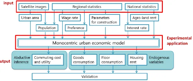
We describe the methodology we use to process remote-sensing data and formulate a monocentric urban economic model. Fig. 13 is a flowchart illustrating the progression of our analysis and the relations between the inputs we use. Satellite images provide objective data from which urban areas can be identified, and numbers for the aggregate populations of large urban zones can be subdivided via grid-based geographical allocation to estimate local populations. Socio-economic data represent the characteristics of urban activities in each city, with the exception of agricultural land rents and interest rates, which are available only on a national level in this study. Given estimates for populations and urban areas, equilibrium values for both endogenous variables (goods consumption, floor consumption, and housing rents) and inferred variables (commuting costs and distances) can be determined. The equilibrium of monocentric urban model is partial, because it abstracts from developments in other markets, like the labor or capital markets. Consequently, the wage rate, the interest
rate and agro-land rent are taken as exogenous. Finally, we validate the applicability of our model by comparing its predictions to observed results.
Figure 13. Analytical flow.
3.1.1 Monocentric urban economic model
As reviewed by Wegener (2004), recent urban models consider highly detailed sets of conditions with many possible variations, thus requiring large amounts of input data. Developing countries are experiencing explosions of urban population, and face the challenges of efficiently managing urban system including conducting socio-economical survey and providing accurate spatially-detailed statistical data. Thus a more primitive model with reduced data requirements for studies in developing countries is highly desirable. The core of the AMM model lies in the bid rent theory, which models tradeoffs between accessibility and land rents in housing market; by simplifying a more complex reality through the assumption of spatial heterogeneity, this model provides insight into the long-term factors influencing urban equilibrium.
Figure 14. The way to fit a real-life city of an irregular shape into the mechanism of monocentric urban model.
Fig. 14 shows the process of how to fit a real-life city of an irregular shape into the mechanism of monocentric urban model. Here we augment the AMM model by adding a building-developer component to separate land and housing markets in analyzing housing consumption. Changes occurring in commuting and lifestyle patterns can be estimated quantitatively by considering shifts in spatial form and economic growth.
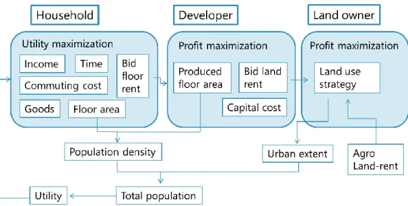
Fig. 15 illustrates the structure of a bid rent-based urban model. The agents in this model consist of households, developers, and absentee landowners, each seeking to maximize utilities or profits. Under given time and budget constraints, with given goods prices and floor rents, households determine their consumption of goods and floors to maximize their utility. A bid floor rent can be calculated when a utility level is given.
Figure 15. Schematic diagram of the bid-rent-based urban model.
Developers use capital and land to produce floors, determining floor areas to maximize profit at a given floor rent. Bid land rent is calculated by assuming zero profits for the developer in a fully competitive market. Landowners determine land-use strategies that maximize profit; for example, they will lend their land to developers if the bid land rent is higher than the land rent for agriculture. Land rent typically decreases as one goes farther from the central business district (CBD), and the decisions of landowners thus determine urban extents (Fig. 16). Population density is calculated by dividing the floor area supplied by the average floor area consumed by a single household.
The total urban population is the product of the population density and the area of the urban region. If the total urban population is provided exogenously, utilities may be adjusted until the population predicted by the model matches the given value.
Figure 16. Definition of urban boundary.
The details of our model formulation and calculation procedures are presented in Appendix A, where we derive several master formulas predicting values of various statistical indices; here we discuss just the key features of these formulas. Our model analyzes past urban features governing the mechanisms of urban formation. We begin by estimating unit commuting cost according to the following equation (the equation number is that given in the Appendix):
1 1 1 4 2 1 1 A A t A A t t A N c x c c x w T w T w T (32) Here N is the total urban population, ct is the generalized unit commuting cost, w isthe wage rate, TA is the total number of hours available for work, commuting, and disposable
(personal) time; xA is the urban radius, and β1, β4 are constants. N, TA, w, β1, and β4 are
obtained from socioeconomic data, while xA is derived from-remote sensing data. We solve
both direct costs for transportation and, travel time and indirect costs associated with factors such as safety and discomfort. In our estimates, unit commuting cost is calculated in each city; in reality, of course, commuting costs vary according to transport mode, time, and location. The estimated cost of commuting may be thought of as an aggregate measure of average travel costs determined by the spatial extent of an urban region. Once ct is obtained,
we can estimate the average commuting distance by equation (33), composite goods consumption by equation (36), average floor consumption by equation (34), floor rent per unit area by equation (35), and disposable time by equation (37).
3.1.2 Definition of “urban area”
We begin by processing Landsat Thematic Mapper (TM) images (U.S. Geological Survey, 2016), which include land-cover information. We use all spectral bands in each dataset to classify land use via the maximum likelihood method with a supervised learning project. The training area of each dataset is selected by visual observation of natural color bands in composite images (bands 1, 2, and 3 for Landsat 7 Enhanced TM and bands 2, 3, and 4 for Landsat 8). Each land-cover unit is then classified into one of three categories: “urban,” “water,” and “cropland and others.” The accuracy of this classification process is verified after its completion.
The UDI developed from ISA was examined to classify urban structures in the proportion of built-up areas in each 1 km × 1 km grid on the basis of 30 m × 30 m urban land cover maps. The urban spatial area was divided into 900 m × 900 m grid units (unit area 0.81 km2). Intra-urban (0.25 < UDI ≤ 1) and ex-urban areas (UDI ≥ 0.25) were distinguished, and
threshold UDI value of 25% has been used in previous studies as a reasonable criterion for identifying boundaries of urban spatial structures and urban–rural divisions (Lu and Weng 2006; Imhoff et al. 2010; Zhou et al. 2014). Within each captured region by Landsat, we identify the largest agglomeration as the primary urban agglomeration for that region. Of course, population boundaries do not coincide with the boundaries of intra-urban areas were different. Therefore, we estimated the population of an intra-urban area on the basis of two assumptions: (1) the population density of ex-urban areas does not change between the two time periods we consider, while (2) the average population density of intra-urban areas does vary from one period to the next. In total, three population densities were estimated using jurisdictional population statistics and intra-urban grids to allocate statistical populations onto grid-based urban spaces. The details of our procedure are discussed in Appendix B.
3.2 Data
3.2.1 Data collection and parameter estimation”
In this study, the mega-city Beijing, the inland metropolis Nanjing, and the medium-sized coastal city Haikou were taken as representative cities to assess the performance of our proposed model in two time periods: 2003 and 2013. The criteria for selecting objectives are urban spatial extent, population size and geography location. The Socioeconomic statistical data (per capita) for each city in each period were obtained from government statistical reports (Beijing Statistical Information Net 2016; Statistics Bureau of Nanjing 2016; Haikou Municipal Government 2016). As input data for determining model parameter values, we considered income, composite goods consumption, usable residential floor area, rent per unit floor area, total housing sales by area, total housing sales by purchase amount, and land-development investments involving residential construction. The average floor area produced
per year was calculated by dividing the total amount paid for all home sales by the average selling price per unit floor area that year. Table 1 shows details on collected statistical data and estimated urban area/ population data. Table 2 presents details estimated parameters.
Table 1. Collected data.
2003 2013
Beijing Nanjing Haikou Beijing Nanjing Haikou Total available hours
(hours/year) 4732 4732 4732 4732 4732 4732
Wage rate
(yuan/hour) 6.7 4.9 4.1 19.3 19.1 11.7
Capital cost (%) 5.3 5.3 5.3 6 6 6
Rent for agricultural use
(yuan/m2) 2.0 2.0 2.0 3.6 3.6 3.6
Estimated urban area
(km2) 3774.6 1073.3 281.8 5641.6 1797.4 455.2 Estimated population
(million) 8.071 2.664 0.723 17.326 5.581 1.697
Table 2. Estimated parameters (p-values are given within parentheses).
2003 2013
Beijing Nanjing Haikou Beijing Nanjing Haikou
z 0.3831 (0.0001) 0.3649 (0.0003) 0.3869 (1e-05) 0.3295 (4.9e-05) 0.3211 (0.0002) 0.3403 (0.0002) s 0.5513 (2.4e-05) 0.5568 (0.0001) 0.5433 (2.7e-06) 0.5845 (7.4e-06) 0.5937 (1.5e-05) 0.5746 (2.6e-05) l 0.0656 0.0783 0.0698 0.086 0.0852 0.0851 0.5015 (7e-04) 0.4568 (0.0072) 0.2641 (0.0006) 0.4870 (0.0028) 0.4165 (0.0014) 0.2701 (0.0007) 0 0.6208 (0.0007) 0.6637 (0.0016) 1.701 (0.0091) 0.2838 (0.0002) 0.7655 (0.0009) 1.8137 (0.0069)
The land-cover images used for each city were obtained from remote-sensing data archives with 30 m × 30 m spatial resolution. The selection criteria for the two datasets were that the datasets must be for the same region with less than 20% cloud cover for the three cities in the two periods. As discussed above, the intra-urban area was defined to be the target urban area. We assumed work times of 8 hours a day, 5 days a week, and 52 weeks a year (Legislative Affairs Office of the State Council P. R. China 1995). The population was estimated using areas extracted for different UDI values together with census data. The wage rate is taken to be an individual’s income divided by that individual’s total work time. There is no authoritative survey on total available time; however, by using empirical methods and deducting the time necessary for basic human functions, total available time was estimated to be 13 hours a day (China National Tourism Administration 2016). Capital costs are estimated based on lending rent figures in the World Development Indicators (World Bank 2013). Land rents at urban boundaries depend on the estimates of the Global Trade Analysis Project and vary with annual lending interest rates given by the World Bank.
Household and developer parameters were estimated using nonlinear regressions from related formulas (for details, see Appendix A) with statistical data from 2002 to 2004 and 2012 to 2014. Work times were fixed to calculate wage rates, and locations were fixed to calculate potential income, although in fact these quantities vary with location in the model. For developer parameters, the produced floor area was calculated by dividing the total money invested by the average selling price per unit floor area. The total money invested includes investments in land and housing development. We assumed that investments were capitalized into building stock and defined the cost flow as the product of the capital stock and the
interest rate. Population densities in intra-urban and ex-urban areas were estimated assuming a constant population density for the ex-urban areas.
Figure 17. Beijing intra-urban area in 2003 (left) and in 2013 (right).
Figure 19. Haikou intra-urban area in 2003 (left) 2013 (right).
3.2.2 Extracting intra-urban areas
Our procedure for extracting intra-urban area was discussed before. Figs. 17 to 19 illustrate the intra-urban areas for each metropolitan zone as extracted from remote-sensing images. The results of our extraction procedure for urban areas, and urban population estimates based on these results, are shown in Table 3.
3.3 Results and analysis
3.3.1 Variation in urban area and population
Both urban population and area have experienced tremendous growth in all three Chinese cities. A comparison of the 2013 and 2003 data shows that in Beijing, Nanjing, and Haikou, the intra-urban area increased by 1.51, 1.67, and 1.61 times, respectively, while the population increased by 2.15, 2.09, and 2.34 times respectively. The population density of the intra-urban area in each city has risen by approximately 900 per km2. The population-density growth coefficient (Table 3) can be interpreted as a measure of the urbanization rate.
Table 3. Citywide average population density and growth coefficients.
Beijing Nanjing Haikou
Ex-urban population density
(1,000 per km2) 0.89 0.63 0.61
Intra-urban population density in 2003
(1,000 per km2) 2.13 2.48 2.57
Intra-urban population density in 2013
(1,000 per km2) 3.07 3.10 3.72
Population density growth coefficient 1.436 1.250 1.452
Population increase and urban expansion are closely interlinked and mutually reinforcing. The total volume of urbanization is greater in Beijing than in Nanjing or Haikou; however, the population density of Beijing appears to be lower than that of the other two cities (Table 3).
The development of new infrastructure and housing construction occupies more territory and leads to a more rapid population sprawl. Conversely, new urban development alleviates exorbitant regional populations and spurs redesign of regional traffic distributions —assuming traffic and housing construction are managed properly—, which is an important consideration for strategic urban planning.
3.3.2 Variation in traffic and residential conditions
As discussed above, average commuting costs and utilities are determined by abductive reasoning from given data on equilibrium population and urban area. Endogenous variables such as goods consumption, floor consumption, and house rents were also calculated.
Simulation results (Table 4) showed that, on average, commuting costs grew considerably compared to the commuting distance. Favorable conditions for infrastructure development in Beijing and Nanjing are ranked among the factors contributing to lower commuting costs; this helps accelerate urban expansion by providing more location options. Our estimated commuting costs include monetary valuations of time loss corresponding to travel distance, which reminds that time spent commuting cannot be neglected in view of its significant effect on residential location choices.
Bar graphs in Fig. 20 and Fig. 21 also display our simulation results.
Table 4. Statistical data and estimated results.
2003 2013
Statistical data Beijing Nanjing Haikou Beijing Nanjing Haikou
Composite goods
consumption (yuan/year) 11123 7725 6607 26275 25647 16856 Average floor consumption
(m2) 18.7 21.1 20.0 31.3 30.2 29.9
Floor rent per unit area
(yuan/m2/year) 51 44 40 67 54 53
Estimated data Beijing Nanjing Haikou Beijing Nanjing Haikou
Average commuting cost
(yuan/km) 0.08 0.12 0.14 0.67 1.41 1.99
Average commuting distance
(km/year) 10977 6138 3146 11121 6153 3175
Composite goods
consumption (yuan/year) 11861 8352 7299 28499 27179 17422 Average floor consumption
(m2) 30.5 27.2 26.7 21.3 36.4 28.5
Floor rent per unit area
(yuan/m2/year) 67 66 49 348 198 153
Disposable time (hours/year) 2557 2600 2528 2607 2621 2538
Figure 20. Simulated results of composite goods consumption, floor rent and floor area consumption per capita.
Figure 21. Simulated results of commuting cost, utility and disposable time per capita.
The deviation from statistical data of the results regarding floor space that emerge from our simulations seems to indicate a poor fit with reality, likely attributable to the effects of policy lag on housing, which creates a supply-demand gap. In this study, the markets for
Composite goods Consumption
(yuan/year)
Floor rent
(yuan/m2/year) Floor area(m2)
0 5,000 10,000 15,000 20,000 25,000 30,000 Be iji ng Be iji ng N an jin g N an jin g Ha ik ou H ai ko u 20032013 20032013 20032013 0 5 10 15 20 25 30 35 40 Be iji ng Be iji ng N an jin g N an jin g H ai ko u H ai ko u 2003 2013 2003 2013 2003 2013 0 50 100 150 200 250 300 350 400 Be iji ng Be iji ng N an jin g N an jin g Ha ik ou Ha ik ou 2003 2013 2003 2013 2003 2013
Utility Disposable time
(hours/year) 2500 2530 2560 2590 2620 2650 Be iji ng Be iji ng N an jin g N an jin g H ai ko u H ai ko u 2003 2013 2003 2013 2003 2013 0 0.5 1 1.5 2 2.5 Be iji ng Be iji ng N an jin g N an jin g H ai ko u H ai ko u 20032013 20032013 20032013 Commuting cost (km/year) 0 1000 2000 3000 4000 5000 6000 7000 Be iji ng Be iji ng N an jin g N an jin g H ai ko u H ai ko u 20032013 20032013 20032013
land and residential housing floor space were cleared in each period (i.e., all assumed variables were optimized immediately), and the estimation errors may be caused by excessive floor rents or land rents. In our estimations, floor rents are affected through housing markets by investments, by the selling price of unit floor area, and by capital costs; however, these quantities may experience time lags. In reality, land-use changes are quite slow compared to changes in interest rates or economic cycles; some urban redevelopment projects take years or decades, and changing residential locations can also take a long time. Housing policies also affect this discrepancy. Local governments provide their own housing policies, including social housing and public housing as well as rent subsidies. These policies obviously restrain the inflation of housing rent. However, our analysis assumes that housing markets operate without policy interference. The impact of such policies will be considered in further studies. At the city level, the increased share of income spent on living expenses implies that city dwellers prefer to live close to their workplace. Effective combinations of traffic and housing policies may lead to more efficient urban management in the population-growth stage.
The increased utility derived from the interaction of goods consumption, usable floor area, and disposable time demonstrates that living standards have improved overall. The total available time (sum of work time, commuting time, and disposable time) was assumed to remain unchanged. Population increase requires urban expansion, which induces changes in travel, work, and disposable time.
The results of this study showed that disposable time increased slightly, implying a decrease in work time. This may indicate individuals’ perceptions of their changing lifestyles amid urban growth and economic development, creating motivation to shorten work times in response to increased wages to maximize overall utility.
For fixed amounts of time devoted to work, individuals would seek to reduce commuting time to increase disposable time. For those who settle in cities, living near workplaces is the preferred means of reducing commuting times. This is consistent with an increased share of income spent on living expenses, demonstrating the need for strategic policy orientations that integrate transportation and housing considerations.
3.3.3 Discussion of the monocentric urban economic model
The monocentric urban model used in this study relies on several important assumptions, whose validity must be addressed. For simplicity, we assumed that urban areas are monocentric structures with homogeneous households and uniform space. With this assumption, urban spaces are symmetric about the CBD and assume an abstract circular shape; this approximation allows us to neglect the effects due to the actual shapes of urban areas. In reality, most cities have complex structures, and the distribution of developed areas always forms noncircular configurations, resulting in eccentric city shapes that extend in specific directions. This is problematic for many existing due to the difficulty of describing distances from the urban core. Random selection of locations in a uniformly homogeneous space leads to a similar, concentric circle structure, which is an urban form described by Alonso (1964).
Associated with the growing its scale, a city appear to be multi-centered. Therefore, it is necessary to discuss the distortions entailed by approximating polycentric cities by monocentric city. If excessive commuting does not occur in a polycentric city, then commuting distances will be shorter and traffic cost estimates higher than in a monocentric model (otherwise, the estimated urban area will be larger than is actually observed). Some
studies have shown that, even if excessive commuting is present, observed commuting distances will be still shorter than values estimated on the basis of the monocentric assumption. Therefore, if traffic costs are set in accordance with current conditions, it is impossible to predict in advance the magnitude of the errors incurred by approximating polycentric cities by monocentric structures when predicting urban radii. In reality, analyses based on polycentric urban models analysis are more trustworthy, and simulations of urban activities in the framework of polycentric urban economic models can always be used to supplement estimates of relevant statistical quantities. This strategy can greatly enhance algebraic calculations in simulations, but also poses the challenge of collecting data in developing countries.
If the distortions produced by monocentric city models are tolerable, then such models offer the potential to provide estimates over a wide range of conditions and scenarios, in view of their reduced data requirements and relatively minimal computational cost. Being equilibrium models, these models are likely to underestimate the scale of urban areas during periods of population decrease, and are thus not useful for examining declining statistical measures for urban areas with falling populations. Nonetheless, in view of the limitations of survey data, the model proposed here is attractive for the straightforward implementation it offers at strategic levels.
3.4 Summary
This chapter considered a classic urban model emphasizing the long-term effects of traffic and residential conditions in an urban landscape. The model is static and simulates the equilibrium structure for a city given certain assumptions. It does not account for the long-term prediction of the housing stock, nor the process of urban change and phenomena such
as gentrification. The model's simplicity helps focus on fundamental factors, which is well suited for the purposes of this paper: as policy support, providing insights into the longer-run determinants of the urban equilibrium, especially for cities that confront the challenge of collecting data.
Population flow into cities requires the development of new infrastructure and housing construction. The proposed model of urban development adapts to changes in spatial layout, for which traffic and housing policies must be managed appropriately. A comparison between observed data and the results of our simulations suggests approaches to solving urban problems through appropriate policy measures. In particular, the advantage of good transport infrastructure is that it accelerates the increase in the number of location choices available to city dwellers, spurring lifestyle changes while restraining the negative impact of urban sprawl. Commuting time must not be neglected because of its significant effect on city dwellers’ location choices.
The deviation from statistical data of the estimates of floor consumption and floor rent produced by our simulation may be attributed to the effects of lag times in housing policy, which create supply-demand gaps. The analysis of this study assumed a pure housing market unaffected by public housing policies. However, local governments in target cities in fact provide various public housing policies which do affect urban formation in practice. Theoretically, living near one’s workplace is the preferred location option, and this is indicated by the increased share of expenditures on housing, implying a tradeoff between commuting time and floor rent. The combination of effective traffic and housing policy may lead to more efficient urban management in the population-growth stage.
Finally, we validated the applicability of our monocentric urban economic model across multiple regions and derived several policy implications concerning urban sprawl. Incorporating remote-sensing data into monocentric urban models is a useful option for applications to developing countries, where spatially-disaggregated data are scarce; further studies of both urban modeling and spatial data acquisition are needed to pursue this possibility.
Chapter 4.
Application II: the model of centrality-based index of a location
In reality, a co-evolution of land use and transportation system can be observed in many cities. When a transit line is implemented on a specific corridor, the presence of this transit line then attracts new residents/businesses and intensifies the land-use, which may then create a need for a higher order transit service on this corridor. This phenomenon is often more acute around transfer stations. It can be speculated that transit network properties may have an effect on the concentration of urban activities in a city. Nevertheless, it is particularly challenging to quantify the relationship between them.
As the study of transportation / land-use interactions is becoming increasingly important in the literature, adopting a network approach could reveal useful properties and effects. As mentioned in literature review, works directly combining network centrality property with distance to amplify its impact in real-life space is still scarce. In this chapter, we develop centrality measures to incorporate actual spatial distance to reflect the importance of a location affected by URT network shape. To meet the demand of mobility, URT system has been developed in most metropolitans, in some case, urban space structure experiences decentralization during the process of its development (Fig. 22). The planning of transportation systems is a multifaceted process that is proved to be extremely complicated because a physical network is hard to upgrade along with the development of new theory and new technology. In this regard, proposing research methods in view point of emerging network science could be particularly valuable to help transportation planners.
Figure 22. Urban evolution from monocentric to polycentric URT development.
4.1 Methodology
Fig. 23 is a flowchart illustrating how we conduct our analysis. Nighttime light images provide objective data used for reflecting economical attraction of a location, and then potential accessibility can be calculated to explain the ease of reaching to economic activity. A centrality-based index of a location is created to understand the importance of a location affected by URT network shape, i.e., amplifying URT network properties to the whole urban area beyond network itself. By integrating this two grid-based properties of a location, the decision to locate in somewhere can be inferred, which is validated by comparison with the distribution of commercial facilities from observed data.
URT in this thesis represents various types of urban rail systems that operates along exclusive right-of-way, whether underground, at grade, or elevated.
Figure 23. Analytical flowchart.
4.1.1 Centrality measures
In graph theory and network analysis, the concept of centrality identifies the most important nodes within a graph, which means the importance of stations when it comes to an URT network. There are many categories of centrality indicators, but the present paper only applies betweenness and closeness to URT network.
a) Betweenness
Betweenness quantifies the number of times a node acts as a bridge along the shortest pathway between two other nodes. Betweenness centrality emphasizes the importance of a node lied on paths as a transfer point between any pairs of nodes, which considers that geographic location has strong influence on flows passing among nodes. Betweenness centrality is also convenience to examine network reliability on the occasion of the happening of dysfunctional nodes or disconnected links and is formulated as follows.
( ) ( ) jk b i j k jk d i C i d
(4-1)Where djk is the number of shortest paths from node j to node k, and djk(i) is the
number of those paths that go through node i.
b) Closeness
Closeness depends on the length of the pathways from a node to all other nodes in the network, and is defined as the inverse total length. Closeness is an indicator that identities how close a station is to all the other stations in terms of a sum of the shortest distances and is formulated as follows. 1 ( ) 1 n c ij j C i d
(4-2) dij= min(xih+ ⋯ + xhj) (4-3)Where dij is the shortest path and h are intermediary nodes on paths between node i
and node j.
4.1.2 Centrality-based index of a Location (CL)
At level of grid cell, we integrate actual distance with centrality by considering the distance decay effect as an exponential function. In terms of betweenness and closeness, the centrality-based accessibility can be described as follow.
𝐶𝐿𝑏(𝑖) = ∑𝑛 𝐶𝑏(𝑖) × 𝑒𝑥𝑝‐𝑚𝑑𝑖𝑗
𝑗=1 (4-4)
𝐶𝐿𝑐(𝑖) = ∑𝑛 𝐶𝑐(𝑖) × 𝑒𝑥𝑝‐𝑚𝑑𝑖𝑗
𝑗=1 (4-5)
Where n represents the number of stations, mdij represents the direct distance (km)
from grid cell i to grid cell j where station is located in.
Figure 24. Illustration of the concept CL (Centrality-based index of a Location).
4.1.3 Potential Accessibility (PA)
Potential accessibility is based on the assumption that the attraction of a destination increases with size, and declines with distance, travel time or cost. Destination size is usually represented by population or economic indicators such as GDP or income.
𝑃𝐴(𝑖) = ∑ { 𝐴𝑇𝑗
∑𝐽𝑗=1𝐴𝑇𝑗
∙ 𝑒𝑥𝑝−𝛼∙𝑐𝑖𝑗}
𝐽