The vaccination program against avian influenza : A mathematical approach (Modeling and Complex analysis for functional equations)

The vaccination

program

against

avian

influenza:

A mathematical

approach

Shingo

Iwami

,

Yasuhiro Takeuchi

Graduate School

_of

Science and Technology, Shizuoka University, Japan

Abstract

It was reported that a vaccination program against avian influenza executed in

China eradicated adominant avian flu virus but led toaprevalenoeofpredominant

avian flu virus. Interestingly, the change of the prevalence could

occur

in other

countries where thevaccination program wasnot executed. The mechanism for the

emergence and prevalenceofpredominant virus isstill unknown. In this study, we

construct and analyze a mathematical model to investigate the mechanism.

1

_Introduction

In China, despite acompukory _{program for the vaccination of all} poultry commencing,

$H5N1$ influenza virus has caused outbreaks in _{poultry in 12 provinces. Epidemiological}

analysisshowed that $H5N1$ influenza viruses

were

_{continued to be perpetuatedinpoultry} in eachoftheprovinces taeted, mainly in domestic duck and

geese.

Interestingly, genetic

analysis revealed that $\bm{t}H6N1$

influenza

variant (Fujit-like) had emerged $\bm{t}d$ become

prevalent variant ineachof the provinces, replacingthose previouslyestablished multiple

sublineages indifferent regionsof southern China. Somedataidicatethat seroconversion

rates

are

still low and that poultry

are

poorly immunized against $FJ$-like viruses, which

suggests that the poultry vaccine currently used in China may only generate very low

neutralizing antibodies to $FJ$-like viruses in comparison to otherpreviously cocirculating

$H5N1$ sublineages _{([9]). This situation can help to select for the FJ-like sublineage in}

poultry. To investigate the change of prevalent strain we propose the following simple

mathematicalmodel: $X_{1}’=(1-p)c-(b+e)X_{1}-(\omega_{1}Y_{1}+\phi_{1}Z_{1})X_{1}$, $V_{1}’=pc-(b+e)V_{1}-\sigma\phi_{1}Z_{1}V_{1}$, (1) $Y_{1}’=\omega_{1}Y_{1}X_{1}-(b+m_{y})Y_{1}$, $Z_{1}’=\phi_{1}Z_{1}(X_{1}+\sigma V_{1})-(b+m_{z})Z_{1}$

.

’This author $i\epsilon$ supportedby ResearchRUowships of the Japan Society for thePromotion ofScience

In the model, $X_{1},$ $V_{1},$ $Y_{1}$ and $Z_{1}$ denote susceptible birds, vaccinated birds against

domi-nant strain, infected birds with dominant avian flu

strain

and infected bird with predom-inant avian flu strain, respectively. The parameter $c$ is the rates at which new birds

are

born. At the beginning of vaccination program, $X_{1}$ directly

moves

to $V_{1}$ by the

vaccina-tion to susceptible birds. However, after

some

vaccinated period, the direct movement may vanish because almost all birds

are

vaccinated. Thereafter, the vaccination is only

administered to the

new

born birds. In order to simplify the vaccination program

we

consider only the vaccination to the

new

born birds because the direct movement by the

vaccination program canbe expressed by

some

cholce ofinitial value. The

new

bom bIrds

are

vaccinated at the rate $0\leq p\leq 1$ and the vaccinated individuals

can

completely pro-$tecthom$ the dominant strain$\bm{t}d$partial protect from the predominant strain at therate

$0\leq 1-\sigma\leq 1$ (for example, $\sigma=0$ represents complete

cross

immunity against dominant

andpredominrt strains). The parameter$b$isthe natural death rate and $e$ isthe dispersal

or

export rate. We consider that only susceptible $\bm{t}d$ vaccinated birds

can

be dispersed

or

exported bmause the avlan flu viruses

can

cause

severe

illness and high mortality in

poultry. Further $m_{y}$ and $m_{z}$

are

the additional death rate mediated by avian flu. The

parameters $\omega_{1}\bm{t}d\phi_{1}$

are

the transmission rate of dominant $\bm{t}d$ predominant avian flu

straio, respectively. For $in8tance$, we can consider that the dominrt avit flu strain

represents current vaccine strain in poultry and the predominant avit flu strain repre-sents FJ-like $virus\infty$ which has emerged and

are

selected when the vaccination program

is executed ([9]).

Rrther the

FJ-like

viruses have already trtsmitted to Hong Kong, Laos, Malaysia

and Thailand, resulting in

anew

trtsmission $\bm{t}d$ outbreak

wave

in Southeast Asia. It

is strangethat the FJ-like viruses become prevalent strain in $n\not\in vaccinated$

area

because

the dominant strain prevailed before the initiation of the vaccination program executed in other

areas.

The mechanism for the

emergenoe

and prevalence oftheFJ-likevirus

over

alarge geographical region within ashort period is still unknown. It is sald that

one

possibility is $\bm{t}$ effect of carrier wild birds: Origins could be traced by $u$sing probes of

various regiooof the

new

isolates andthis analysisindicated many contained regionsthat

traced back to wild bird isolates in Hong Kong in 2003, or isolates from northern China

in

2003.

Thesedataindicate wild bir&are responsiblefor the transport andtransmission of the evolving $H5N1$

.

However, in this paper,

we

investigate the another possibility of

the emergence andprevalence by

amathematical

model. Based

on

concerns

about highly

pathogenic avianinfluenza $H5N1$ virus and its potential to

cause

illness in humans, CDC

and the U.S. Department ofAgriculturehave taken steps toprevent importation ofbirds

and unprocessed bird products Bom countries with the virus in domestic poultry ([4]). However it is impossible for government to control the importation completely because

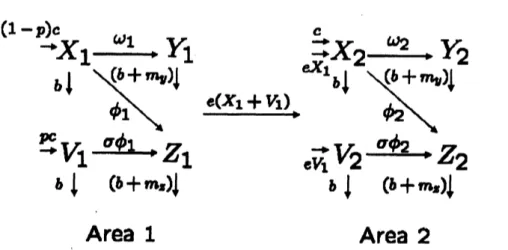
Area1

Area

2

Figure 1: Model schematic showing the vaccination program and the illegal trade or dispersal

in poultryBom Area 1 to Area2

of

some

smuggler. For example, in

some

outbreaks, the tendency to hide

or

smuggle

especially valuable birds, such

as

fighting cocks,

can

also help maintain the virus in the

environment

or

contribute to its further geographical spread ([10]). Therefore,

we

have

to consider the

effect

of the export

or

dispersal of domesticpoultry. Remember that only

susceptible and vaccinatedbirds

can

bedispersedorexportedbecausethe avian fluviruses

can

cause

severe

illness and high mortality in poultry. We

assume

that the vaccination

program is executed in Area 1 (such as China) but the program is not executed in Area

2 (such

as

Malaysia, Vietnam and Thailand) and both susceptible _{and vaccinated birds}

export or disperse from

Area

1 to Area 2 (see Fig. 1). These assumptions lead to the

following mathematical model:

$X_{1}’=(1-p)c-(b+e)X_{1}-(\omega_{1}Y_{1}+\phi_{1}Z_{1})X_{1}$, $V_{1}’=pc-(b+e)V_{1}-\sigma\phi_{1}Z_{1}V_{1}$, $Y_{1}’=\omega_{1}Y_{1}X_{1}-(b+m_{y})Y_{1}$, $Z_{1}’=\phi_{1}Z_{1}(X_{1}+\sigma V_{1})-(b+m_{z})Z_{1}$, (2) $X_{2}’=c+eX_{1}-bX_{2}-(\omega_{2}Y_{2}+\phi_{2}Z_{2})X_{2}$, $V_{2}=eV_{1}-bV_{2}-\sigma\phi_{2}Z_{2}V_{2}$, $Y_{2}^{j}=\omega_{2}Y_{2}X_{2}-(b+m_{y})Y_{2}$, $Z_{2}’=\phi_{2}Z_{2}(X_{2}+\sigma V_{2})-(b+m_{z})Z_{2}$

.

Inthemodel,$X_{1},$ $V_{i},$$Y_{1}$and $Z_{i}$denote susceptiblebirds, vaccinated birdsagainstdominant

strain, infected birds with dominant avian flu strain and infected bird with predominant

avian flu strain in Area $i(i=1,2))$ respectively. The parameters $w_{i}$ and $\phi_{i}$

are

the

transmission rate of

dominant

and predominant avian flu strains in Area $i$, respectively.

discussion of this model,

see

[8].

2

Mathematical properties

In order to investigate thechange ofprevalencestrain in Area 1 and

2

by thevaccination

program

we

have to demonstrate the mathematical properties of model (2). We remark that thedynamics in Area 1

are

independent of those in

Area

2. Therefore

we can

obtain

the dynamical properties in

Area

1 from only model (1).

Once we

obtain the properties

in Area 1,

we can

easilyunderstand those inArea 2 by a similar method in $Theo7em$ A.$l$

of [5].

2.1

The disease

transmission in Area

1

To understandthedynamicsofthedisease transmission inArea 1

we

firstly analyzemodel

(1) and divide the analysis into three situations concerned with the vaccination rate

as

follows;

$(a)$ No vaccination program; $p=0$ in

Area

1

If the vaccination rate $p=0$ (No vaccination program), then model (1) is $X_{1}’=c-(b+e)X_{1}-(\omega_{1}Y_{1}+\phi_{1}Z_{1})X_{1}$,

$V_{1}’=-(b+e)V_{1}-\sigma\phi_{1}Z_{1}V_{1}$,

(3)

$Y_{1}’=\omega_{1}Y_{1}X_{1}-(b+m_{y})Y_{1}$,

$Z_{1}’=\phi_{1}Z_{1}(X_{1}+\sigma V_{1})-(b+m_{z})Z_{1}$

.

It is clear that $\lim_{tarrow\infty}V_{1}(t)=0$and this syst$em$hasthefollowingthree possible equilibria:

$E_{1}^{n0}=(X_{1}^{n0},0,0,0)$, where $X_{1}^{n0}= \frac{c}{b+e}$;

$E_{1}^{nd}=,$ $(X_{1}^{nd}, 0, Y_{1}^{nd}, 0)$, where $X_{1}^{nd}= \frac{b+m_{y}}{\omega_{1}},$ $Y_{1}^{nd}= \frac{c-(b+e)X_{1}^{nd}}{w_{1}X_{1}^{nd}}$; $E_{1}^{\mathfrak{n}p}=(X_{1}^{np}, 0,0, Z_{1}^{np})$, where $X_{1}^{np}= \frac{b+m_{z}}{\phi_{1}},$ $Z_{1}^{np}= \frac{c-(b+e)X_{1}^{np}}{\phi_{1}X_{1}^{np}}$

.

Note that model (3) is typical competitive system for multiple infectious strains which leads tocompetitiveexclusion $([1]-[3], [7])$

.

Thedynamicsof(3) arecompletelydetermined

by the so-called basic reproductive number of the dominant and predominant strains,

respectively ([7]):

Clearly $E_{1}^{n0}$ always exists, $E_{1}^{nd}$ exists iff _{$R_{1}^{nd}>1$} and $E_{1}^{np}$ exists iff$R_{1}^{np}>1$

.

Further, to

simply understand

a

concept ofcompetitionbetween the strainswe introduce theanother

basic reproductive numbers ([6]):

$\overline{R}_{1}^{nd}=\frac{\omega_{1}}{b+m_{\nu}}X_{1}^{np}$, $\overline{R}_{1}^{np}=\frac{\phi_{1}}{b+m_{z}}X_{1}^{nd}$

.

We remark that $R_{1}^{\mathfrak{n}d}(R_{1}^{\mathfrak{n}p})$ represents

an

average

number of the infected birds with the

dominant (predominant) avian flu by

a

single infected bird with the dominant

(predomi-nant) strainunder the conditionthat all birds

are

susceptible, but $\overline{R}_{1}^{nd}(\overline{R}_{1}^{np})$ is the basic

reproduction number after

a

spread of predominant (dominant) strain in the bird world.

Note that $\overline{R}_{1}^{nd}\overline{R}_{1}^{\mathfrak{n}p}=1$

.

Further these basic reproductive numbers have the following

relations:

Remark

2.1.

$ffi_{1}>R_{1}^{np}(R_{1}^{np}>R_{1}^{nd})$ is equivalent

to

$\overline{R}_{1}^{np}<1(\overline{R}_{1}^{nd}<1)$ and $\overline{R}_{1}^{nd}<1$

$(\overline{R}_{1}^{np}<1)$ is equivalent to $\overline{R}_{1}^{np}>1(\overline{R}_{1}^{nd}>1)$

.

Thedynamical properties ofmodel (3)

are

given by the following theorem:

Theorem 2.1. (i)

_If

$R_{1}^{nd}\leq 1$ and $R_{1}^{np}\leq 1$, then $E_{1}^{\mathfrak{n}0}$ is globally asymptotically

sta-ble (GAS) which means that the orbit converges to the equilibrium as $tarrow\infty$

for

arbitrary initial point.

(ii)

_If

$R_{1}^{nd}>1$ and$\overline{R}_{1}^{np}<1$, then $E_{1}^{nd}$ is GAS.

(iii)

_If

$R_{1}^{np}>1$ and $\overline{R}_{1}^{\mathfrak{n}d}<1$, then $E_{1}^{np}$ ,is GAS.

The proofs ofthis Theorem

are

given in [7] (see its Theorem 3.1.).

$(b)$ Complete vaccination program: _$p=1$ in Area 1

Ifthe vaccination rate $p=1$ (Completevaccination program), then model (1) is

$X_{1}’=-(b+e)X_{1}-(\omega_{1}Y_{1}+\phi_{1}Z_{1})X_{1}$, $V_{1}’=c-(b+e)V_{1}-\sigma\phi_{1}Z_{1}V_{1}$,

(4)

$Y_{1}’=\omega_{1}Y_{1}X_{1}-(b+m_{y})Y_{1}$,

$Z_{1}’=\phi_{1}Z_{1}(X_{1}+\sigma V_{1})-(b+m_{z})Z_{1}$

.

It is clear that $\lim_{tarrow\infty}X_{1}(t)=0$and $\lim_{tarrow\infty}Y_{1}(t)=0$ and this system has the following

two equilibria:

$E_{1}^{\omega}=(0, V_{1}^{\infty},0,0)$, where $V_{1}^{c0}= \frac{c}{b+e}$;

This system (4) is essentially 2-dimensional and the dynamics is clear ([5]). The basic reproductive number of predominant strain is given by

$R_{1}^{\varphi}= \frac{\sigma\phi_{1}}{b+m_{l}}V_{1}^{c0}$

.

Clearly $E_{1}^{c0}$ always exists and $E_{1}^{q}$ exists iff $R_{1}^{\varphi}>1$

.

The dynamical properties of model

(4)

are

given by the following theorem:

Theorem 2.2. (i)

_If

$R_{1}^{\varphi}\leq 1$, then $E_{1}^{\text{\’{a}})}$ is GAS.

$(i,i)$

If

ROP

$>1$, then $E_{1}^{\varphi}$ is GAS.

The proofs of this Theorem

are

givenin [5] (see its Theorems 3.1.).

$(c)$ Incomplete vaccination $pr^{\backslash }ogmm;0<p<1$ in

Area

1

If the vaccination rate

$0<p<1$

(Incomplete vaccination program), then

we

have to

consider system (1) directly. This system has the following four possible equilibria:

$E_{1}^{i0}=(X_{1}^{i0}, V_{1}^{i0},0,0)$, where $X_{1}^{i0}= \frac{(1-p)c}{b+e},$ $V i^{0}=\frac{pc}{b+e}$;

$E_{1}^{u}=(X_{1}^{u}, V_{1}^{id}, Y_{1}^{id}, 0)$, where $X_{1}^{id}= \frac{b+m_{y}}{\omega_{1}},$ $V_{1}^{id}= \frac{pc}{b+e},$ $Y\dot{i}^{d}=\frac{(1-p)c-(b+e)X_{1}^{id}}{w_{1}X\dot{i}^{d}}$;

$E_{1}^{ip}=(X_{1}^{ip}, V_{1}^{ip}, 0,\dot{Z}_{1}^{p})$, where _{$X_{1}^{1p}= \frac{(1-p)c}{b+e+\phi_{1}Z_{1}^{ip}},$}

$V_{1}^{1p}= \frac{pc}{b+e+\sigma\phi_{1}Z\dot{i}^{p}}$

and $Z_{1}^{ip}$ is the unique root of the following equation:

$\frac{\phi_{1}(1-p)c}{b+e+\phi_{1}Z_{1}}+\frac{\sigma\phi_{1}pc}{b+e+\sigma\phi_{1}Z_{1}}=b+m_{z}$ ; (5)

$Ei^{+}=(X_{1}^{i+}, V_{1}^{i+}, Y_{1}^{i+}, Z_{1}^{i+})$, where $X_{1}^{i+}= \frac{b+m_{y}}{\omega_{1}}$, $V_{1}^{1+}= \frac{1}{\sigma}(\frac{b+m_{z}}{\phi_{1}}-\frac{b+m_{y}}{w_{1}})$ ,

$Y_{1}^{i+}= \frac{1}{w_{1}}\{\frac{(1-p)c-(b+e)X_{1}^{i+}}{X_{1}^{i+}}-\phi_{1}z_{1}^{i+}\},$ $Z_{1}^{i+}= \frac{pc-(b+e)V\dot{i}^{+}}{\sigma\phi_{1}V_{1}^{i+}}$

.

We also introduce the two basic reproductive numbers of dominant and predominant strains;

$R_{1}^{1d}= \frac{w_{1}}{b+m_{\nu}}X_{1}^{i0}$, $R_{1}^{ip}= \frac{\phi_{1}}{b+m_{z}}X_{1}^{i0}+\frac{\sigma\phi_{1}}{b+m_{z}}V_{1}^{i0}$,

The meaningofthesenumbersisthe

same

as

$R_{1}^{nd},$ $R_{1}^{np},\overline{R}_{1}^{nd}$ and$\overline{R}_{1}^{np}$ in $(a)$

.

It isclear that

$E_{1}^{i0}$ always exists and $E_{1}^{id}$ exists iff _{$R_{1}^{id}>1$}

.

From equation (5), the existence condition

of $E_{1}^{ip}$ is given by

$b+m_{z}< \frac{\phi_{1}(1-p)c+\sigma\phi_{1}pc}{b+e}\Leftrightarrow 1<R_{1}^{ip}$

.

Further, let $F$ be the following function of$X_{1}$:

$F(X_{1})=(b+e) \phi_{1}(1-\frac{1}{\sigma})X_{1}^{2}-\{(b+e)(b+m_{z})(1-\frac{1}{\sigma})+\phi_{1}c\}X_{1}+(1-p)c(b+m_{z})$

.

Then

we

obtain the following existence condition of$E_{1}^{i+}$;

$\frac{b+m_{z}}{\phi_{1}}-\frac{pc\sigma}{b+e}<X_{1}^{i+}<\frac{b+m_{z}}{\phi_{1}},$ $0<F(X_{1}^{i+})$

.

Since $0<F(O),$ $0>F( \frac{b+m}{\phi_{1}})$ and $F”(X_{1})<0$we

can

obtain the following relation;

$\frac{b+m_{z}pc\sigma}{\phi_{1}b+e}<X_{1}^{i+}<\frac{b+m_{z}}{\phi_{1}},$ $0<F(X_{1}^{i+}) \Leftrightarrow\max\{0,$ $\frac{b+m_{z}}{\phi_{1}}-\frac{pc\sigma}{b+e}\}<x\dot{i}^{+}<X_{1}^{*}$

where $xi$ is the larger root of$F(X_{1})=0$

.

Fhrom straightforward but tedious calculations,

we can

evaluate $X_{1}^{*}=x\dot{i}^{p}$

.

This implies that

$\max\{0,$ $\frac{b+m_{z}}{\phi_{1}}-\frac{pc\sigma}{b+e}\}<x\dot{i}^{+}<X_{1}^{*}\Leftrightarrow 1<\overline{R}_{1}^{u},1<\overline{R}_{1}^{1p}$

.

In this way,

we

can

conclude the existence conditions of these equilibria in the following lemma.

Lemma 2.1. (i) $E_{1}^{i0}$ always enists in$\mathbb{R}_{+}^{4}$

.

(ii) $E_{1}^{u}$ exists in $\mathbb{R}_{+}^{4}$

iff

$1<R_{1}^{u}$

.

(iii) $E_{1}^{ip}$ exists in$\mathbb{R}_{+}^{4}$

iff

$1<R_{1}^{ip}$

.

(iv) $E_{1}^{i+}$ exists in $\mathbb{R}_{+}^{4}$

iff

$1<\overline{R}_{1}^{u}$ and $1<\overline{R}_{1}^{1p}$.

Here

we

have to note the relation between the basic reproductive numbers in the following Lemma 2.2.

Lemma 2.2. $\overline{\dot{H}}_{1}^{d}<1<R_{1}^{u}$ and$\overline{R}_{1}^{ip}<1<R_{1}^{ip}$

can

not hold simultaneously.

Remark 2.2. Lemma 2.2

can

be proved directly by tedious and complex analysis but it

will be clear in Theorem 2.$S$

.

Theorem 2.3. (i)

_If

$R_{1}^{id}\leq 1$ and$R_{1}^{ip}\leq 1$, then $E_{1}^{i0}$ is GAS.

(ii)

_If

$R_{1}^{id}>1$ and$\overline{R}_{1}^{ip}\leq 1$, then $E_{1}^{u}$ is GAS.

(iii)

_If

$R_{1}^{ip}>1$ and$\overline{R}_{1}^{id}\leq 1$, then $E_{1}^{1p}$ is GAS.

(iv)

_If

$\overline{R}_{1}^{u}>1$ and $\overline{R}_{1}^{ip}>1$, then $\dot{p}_{1}+$ is GAS.

Proof.

(i) Let

us

consider the Lyapunov function

$V_{0}=X_{1}-X\dot{i}^{0}\log X_{1}+V_{1}-V_{1}^{10}$log$V_{1}+Y_{1}+Z_{1}$

.

.We have

$\dot{V}_{0}=(X_{1}-X_{1}^{i0})t\frac{(1-p)c}{X_{1}}-(b+e)-\omega_{1}Y_{1}-\phi_{1}z_{1}\}+(V_{1}-V_{1}^{10})t\frac{pc}{V_{1}}-(b+e)-\sigma\phi_{1}z_{1}\}$

$+Y_{1}\{w_{1}X_{1}-(b+m_{y})\}+Z_{1}\{\phi_{1}(X_{1}+\sigma V_{1})-(b+m_{z})\}$

$=(1-p)c(2- \frac{X_{1}^{10}}{X_{1}}-\frac{X_{1}}{X_{1}^{10}})+pc(2-\frac{V_{1}^{i0}}{V_{1}}-\frac{V_{1}}{V_{1}^{i0}})+w_{1}Y_{1}(X_{1}|0-\frac{b+m_{y}}{\omega_{1}})$

$+ \phi_{1}Z_{1}(X_{1}^{i0}+\sigma V\dot{i}^{0}-\frac{b+m_{z}}{\phi_{1}})$

.

We remark that $X_{1}^{i0}-(b+m_{y})/\omega_{1}\leq 0$iff$\dot{R}_{1}^{d}\leq 1$ and $x\dot{i}^{0}+\sigma V\dot{i}^{0}-(b+m_{z})/\phi_{1}\leq 0$ iff $R_{1}^{ip}\leq 1$

.

Further it is clear that

$2- \frac{X_{1}^{l0}}{X_{1}}-\frac{X_{1}}{X_{1}^{i0}}\leq 0$, $2- \frac{V_{1}^{\dot{|}0}}{V_{1}}-\frac{V_{1}}{V_{1}^{i0}}\leq 0$

because the arithmetic

mean

is larger than,

or

equals to the geometric

mean.

Therefore

$\dot{V}_{0}\leq 0$because $R_{1}^{id}\leq 1$ and$R\dot{i}^{p}\leq 1$, and

we

can

conclude that by theLyapunov-LaSalle’s

invariance principle, all the trajectories of(1) converges to $E_{1}^{i0}$

.

(ii) Let

us

consider the Lyapunov function

$V_{d}=X_{1}-X_{1}^{u}$log$X_{1}+V_{1}-V_{1}^{id}\log V_{1}+Y_{1}-Y_{1}^{u}$log$Y_{1}+Z_{1}$

.

Then

$\dot{V}_{d}=(X_{1}-X_{1}^{1d})\{\frac{(1-p)c}{X_{1}}-(b+e)-w_{1}Y_{1}-\phi_{1}z_{1}\}+(V_{1}-V_{1}^{id})t^{\frac{pc}{V_{1}}-(b+e)-\sigma\phi_{1}Z_{1}}\}$

$+(Y_{1}-Y_{1}^{u})\{w_{1}X_{1}-(b+m_{y})\}+Z_{1}\{\phi_{1}(X_{1}+\sigma V_{1})-(b+m_{z})\}$

.

Since $b+e=(1-p)c/X_{1}^{u}-w_{1}Y_{1}^{u}=pc/V_{1}^{u}$ and $b+m_{y}=w_{1}X_{1}^{u}$,

we

can

evaluate

$\dot{V}_{d}=(1-p)c(2-\frac{X_{1}^{id}}{X_{1}}-\frac{X_{1}}{X_{1}^{id}})+pc(2-\frac{V_{1}^{u}}{V_{1}}$ 一 $\frac{V_{1}}{V_{1}^{id}})$

We remark that $\phi_{1}(X_{1}^{id}+\sigma V_{1}^{id})-(b+m_{z})\leq 0$iff$\overline{R}_{1}^{ip}\leq 1$

.

In the similar manner,

we

can

show that $\dot{V}_{d}\leq 0$ because $\overline{R}_{1}^{ip}\leq 1$

.

This completesthe proof.

(iii) Let

us

consider the Lyapunov function

$V_{p}=X_{1}-X_{1}^{1p}$log$X_{1}+V_{1}-V_{1}^{ip}$log$V_{1}+Y_{1}+Z_{1}-Z_{1}^{ip}$log$Z_{1}$.

We have

$\dot{V}_{p}=(X_{1}-X_{1^{p}}^{j})t\frac{(1-p)c}{X_{1}}-(b+e)-\omega_{1}Y_{1}-\phi_{1}z_{1}\}+(V_{1}-V_{1}^{1p})t\frac{pc}{V_{1}}-(b+e)-\sigma\phi_{1}z_{1}\}$

$+Y_{1}\{\omega_{1}X_{1}-(b+m_{y})\}+(Z_{1}-Z_{1}^{ip})\{\phi_{1}(X_{1}+\sigma V_{1})-(b+m_{z})\}$

.

Since $b+e=(1-p)c/X_{1}^{ip}-\phi_{1}Z\dot{i}^{p}=pc/Vi^{p}-\sigma\phi_{1}^{f\dot{f}_{1}^{p}}$ and $b+m_{z}=\phi_{1}(X\dot{i}^{p}+\sigma Vi^{p})$,

we

can

evaluate

$\dot{V}_{p}=(1-p)c(2-\frac{X_{1}^{ip}}{X_{1}}-\frac{X_{1}}{x\dot{i}^{p}})+pc(2-\frac{V_{1}^{ip}}{V_{1}}-\frac{V_{1}}{V_{1}^{ip}})+w_{1}Y_{1}(X_{1}^{ip}-\frac{b+m_{\nu}}{w_{1}})$

.

We remark that $\omega_{1}X_{1}^{ip}-(b+m_{y})\leq 0$ iff$\overline{R}_{1}^{u}\leq 1$

.

In the similar manner,

we

can

show

that $\dot{V}_{p}\leq 0$ because $\overline{R}_{1}^{u}\leq 1$

.

This completes the proof.

(iv) Let

us

consider the Lyapunov function

$V_{+}=X_{1}-X_{1}^{1+}\log X_{1}+V_{1}-V_{1}^{i+}\log V_{1}+Y_{1}-Yi^{+}$ log$Y_{1}+Z_{1}-Z\dot{i}^{+}\log Z_{1}$

.

Then

$\dot{V}_{+}=(X_{1}-X_{1}^{1+})\{\frac{(1-p)c}{X_{1}}-(b+e)-\omega_{1}Y_{1}-\phi_{1}z_{1}\}+(V_{1}-V_{1}^{i+})\{\frac{pc}{V_{1}}-(b+e)-\sigma\phi_{1}z_{1}\}$

$+(Y_{1}-Y_{1}^{i+})\{w_{1}X_{1}-(b+m_{\nu})\}+(Z_{1}-Z_{1}^{1+})\{\phi_{1}(X_{1}+\sigma V_{1})-(b+m_{z})\}$

.

Since $b+e=(1-p)c/X_{1}^{i+}-w_{q}Y_{1}^{i+}-\phi_{1}Z_{1}^{i+}=pc/V\dot{i}^{+}-\sigma\phi_{1}\dot{Z}_{1}^{+},$$b+m_{y}=\omega_{1}X\dot{i}^{+}$ and $b+m_{z}=\phi_{1}(X\dot{i}^{+}+\sigma V_{1}^{1+})$,

we

can

evaluate

$\dot{V}_{+}=(1-p)c(2-\frac{X_{1}^{1+}}{X_{1}}-\frac{X_{1}}{x\dot{i}^{+}})+pc(2-\frac{V\dot{i}^{+}}{V_{1}}$一 $\frac{V_{1}}{V\dot{i}^{+}})\leq 0$

.

This completes the proof. $\square$

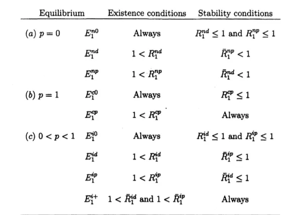
We

can

completely classifythe dynamics of model (1) by the basic reproductive

num-bers. Table 1 summarizes theexistence and stability conditions of the equilibria in

model

Equilibrium Existence conditions Stability conditions

$(a)p=0$ $E_{1}^{n0}$ Always $R_{1}^{nd}\leq 1$ and $R_{1}^{np}\leq 1$

$E_{1}^{nd}$ $1<R_{1}^{nd}$ $R_{1}^{np}<1$

$E_{1}^{np}$ $1<R_{1}^{np}$ $\overline{R}_{1}^{nd}<1$

$(b)p=1$ $E_{1}^{c0}$ Always

ROP

$\leq 1$

$E_{1}^{\varphi}$ $1<R_{1}^{\varphi}$ Always

$(c)0<p<1$ $E_{1}^{i0}$ Always $\dot{H}_{1}^{d}\leq 1$ and $R_{1}^{ip}\leq 1$

$E_{1}^{u}$ $1<R_{1}^{d}$ $\overline{R}_{1}^{ip}\leq 1$

$f\dot{f}_{1}^{p}$ $1<R_{1}^{ip}$ $\overline{R}_{1}^{u}\leq 1$

$E_{1}^{\dot{2}+}$ $1<\overline{R}_{1}^{u}$ and $1<\overline{R}_{1}^{ip}$ Always

Table 1: The existence and stability condition of the equilibria in model (1)

2.2

The

disease

transmission in Area

2

From theclassification ofthedynamics of model (1) in Table 1,

we

can easily understand those in Area2 byanalyzingmodel (2). Fromthe

convergence

theorem (see Theorem A.l of [5]), the global behavior of model (2) is determined by the reduced system;

$X_{2}’=c+eX_{1}^{l}-bX_{2}-(w_{2}Y_{2}+\phi_{2}Z_{2})X_{2}$, $V_{2}’=eV_{1}^{*}-bV_{2}-\sigma\phi_{2}Z_{2}V_{2}$,

(6)

$Y_{2}’=\omega_{2}Y_{2}X_{2}-(b+m_{y})Y_{2}$,

$Z_{2}’=\phi_{2}Z_{2}(X_{2}+\sigma V_{2})-(b+m_{z})Z_{2}$,

where $X_{1}^{*}$ and $V_{1}^{*}$ represent

a

corresponding equilibrium in model (1). Let $a_{1}=c+eX_{1}^{l}$

and $a_{2}=eV_{1}^{*}$, and consider $a_{1},$ $a_{2}$

as

any nonnegative constants. Then model (6)

can

be

considered

as a

special

case

ofmodel (1) with $c=a_{1}+a_{2},$ $p=a_{2}/(a_{1}+a_{2})$ and $e=0$

.

We also divide the analysis into three situations concerned with the vaccination rate

as

$(a)$ No vaccination program: _$p=0$ in Area 1

If the vaccination rate$p=0$ (No vaccination program) in Area 1, then model (6) is

$X_{2}’=c+eX_{1}^{*}-bX_{2}-(\omega_{2}Y_{2}+\phi_{2}Z_{2})X_{2}$,

$V_{2}’=-bV_{2}-\sigma\phi_{2}Z_{2}V_{2}$,

(7)

$Y_{2}’=\omega_{2}Y_{2}X_{2}-(b+m_{y})Y_{2}$,

$Z_{2}’=\phi_{2}Z_{2}(X_{2}+\sigma V_{2})-(b+m_{z})Z_{2}$

.

It is clear that $\lim_{tarrow\infty}V_{2}(t)=0$andthis system has thefoUowingthree possible$e$quilibria: $E_{2}^{n0}=(X_{2}^{n0},0,0,0)$, where $X_{2}^{n0}= \frac{c+eX_{1}^{*}}{b};$

$E_{2}^{nd}=(X_{2}^{nd}, 0, Y_{2}^{nd},0)$, where $X_{2}^{nd}= \frac{b+m_{y}}{\omega_{2}},$ $Y_{2}^{nd}= \frac{c+eX_{1}^{*}-bX_{2}^{nd}}{\omega_{2}X_{2}^{nd}}$;

$E_{2}^{np}=(X_{2}^{np},0,0, Z_{2}^{np})$, where $X_{2}^{np}= \frac{b+m_{z}}{\phi_{2}}$, $Z_{2}^{np}= \frac{c+eX_{1}^{*}-bX_{2}^{np}}{\phi_{2}X_{2}^{np}}$

.

Here $X_{1}^{*}$ represents a corresponding one of $X_{1}^{n0},$ $X_{1}^{nd}$

or

$X_{1}^{np}$

.

IFMrther this model is

essentially

same

asmodel (3) andthedynamicscanbecompletelydecidedbythe following

basic reproductive numbers:

$R_{2}^{nd}= \frac{w_{2}}{b+m_{y}}X_{2}^{n0}$, $R_{2}^{np}= \frac{\phi_{2}}{b+m_{z}}X_{2}^{n0}$, $\overline{R}_{2}^{nd}=\frac{w_{2}}{b+m_{y}}X_{2}^{np}$, $\overline{R}_{2}^{np}=\frac{\phi_{2}}{b+m_{z}}X_{2}^{nd}$

.

Clearly $E_{2}^{n0}$ always exists, $E_{2}^{nd}$ exists iff$R_{2}^{nd}>1$ and $E_{2}^{np}$ exists iff$R_{2}^{np}>1$

.

The dynamical properties of model (7)

are

given by the following theorem: Theorem 2.4. (i)

_If

$R_{2}^{nd}\leq 1$ and $R_{2}^{np}\leq 1$, then $E_{2}^{n0}$ is GAS.

(ii)

_If

$R_{2}^{nd}>1$ and $\overline{R}_{2}^{np}<1$, then $E_{2}^{nd}$ is GAS.

(iii)

_If

$R_{2}^{np}>1$ and $\overline{R}_{2}^{nd}<1$, then $E_{2}^{np}$ is GAS.

The proofs ofthis $Th\infty rem$ are given in [7] (see its Theorem 3.1.). $(b)$ Complete vaccination program: _$p=1$ in Area 1

If the vaccination rate $p=1$ _{(Complete vaccination} program) in Area 1, then model (6)

is $X_{2}’=c-bX_{2}-(w_{2}Y_{2}+\phi_{2}Z_{2})X_{2}$, $V_{2}’=eV_{1}^{*}-bV_{2}-\sigma\phi_{2}Z_{2}V_{2}$, (8) $Y_{2}’=w_{2}Y_{2}X_{2}-(b+m_{y})Y_{2}$, $Z_{2}’=\phi_{2}Z_{2}(X_{2}+\sigma V_{2})-(b+m_{z})Z_{2}$

.

This system has the following four possible equilibria:

$E_{2}^{c0}=(X_{2}^{c0}, V_{2}^{c0},0,0)$, where $X_{2}^{\theta}= \frac{c}{b},$ $V_{2}^{\theta}= \frac{eV_{1}^{*}}{b};$

$E_{2}^{cd}=(X_{2}^{d}, V_{2}^{cd},Y_{2}^{cd}, 0)$, where $X_{2}^{cd}= \frac{b+m_{\nu}}{\omega_{2}},$ $V_{2}^{cd}= \frac{eV_{1}^{*}}{b},$ $Y_{2}^{cd}= \frac{c-bX_{2}^{cd}}{w_{2}X_{2}^{cd}}$; $E_{2}^{\varphi}=(X_{2}^{\varphi}, V_{2}^{\varphi},0, Z_{2}^{\varphi})$, where $X_{2}^{q}= \frac{c}{b+\phi_{2}Z_{2}^{\varphi}},$ $V_{2}^{\varphi}= \frac{eV_{1}^{*}}{b+\sigma\phi_{2}Z_{2}^{\varphi}}$

and $Z_{2}^{\varphi}$ is theunique root of the following equation:

$\frac{\phi_{2}c}{b+\phi_{2}Z_{2}}+\frac{\sigma\phi_{2}eV_{1}^{*}}{b+\sigma\phi_{2}Z_{2}}=b+m_{z}$;

$E_{2}^{c+}=(X_{2}^{c+}, V_{2}^{c+},Y_{2}^{c+}, Z_{2}^{c+})$, where $X_{2}^{c+}= \frac{b+m_{y}}{\omega_{2}},$ $V_{2}^{c+}= \frac{1}{\sigma}(\frac{b+m_{z}}{\phi_{2}}-\frac{b+m_{\nu}}{\omega_{2}})$ ,

$Y_{2}^{c+}=\frac{1}{\omega_{2}}(\frac{c-bX_{2}^{c+}}{X_{2}^{c+}}-\phi_{2}z_{2}^{c+}),$ $Z_{2}^{c+}= \frac{eV_{1}^{l}-bV_{2}^{c+}}{\sigma\phi_{2}V_{2}^{c+}}$

.

Here $V_{1}^{*}$ represents

a

corresponding

one

of $V_{1}^{\infty}$

or

$V_{1}^{q}$

.

This model is also essentially

same

as

model (1) and the dynamics can be completely decided by the following basic reproductive numbers:

$R_{2}^{d}= \frac{\omega_{2}}{b+m_{\nu}}X_{2}^{\theta}$

,

$R_{2}^{q}= \frac{\phi_{2}}{b+m_{z}}X_{2}^{\omega}+\frac{\sigma\phi_{2}}{b+m_{z}}V_{2}^{\theta}$

,

$\overline{R}_{2}^{d}=\frac{w_{2}}{b+m_{\nu}}X_{2}^{\varphi}$, $\overline{R}_{2}^{\wp}=\frac{\phi_{2}}{b+m_{z}}X_{2}^{cd}+\frac{\sigma\phi_{2}}{b+m_{l}}V_{2}^{d}$

.

We

can

also conclude the existence conditions of these equilibria

as same

as

model (1) in the following lemma.

Lemma 2.3. (i) $E_{2}^{d1}$ always exists in $\mathbb{R}_{+}^{4}$

.

(ii) $E_{2}^{d}$ exists in $\mathbb{R}_{+}^{4}$

iff

$1<R_{2}^{d}$

.

(iii) $E_{2}^{\varphi}em\dot{s}ts$ in $\mathbb{R}_{+}^{4}$

iff

$1<R_{2}^{\varphi}$

.

(iv) $E_{2}^{c+}e$vists in$\mathbb{R}_{+}^{4}$

iff

$1<\overline{R}_{2}^{d}$ and $1<\overline{R}_{2}^{\varphi}$

.

Further

we

also remark that $\overline{R}_{2}^{d}<1<R_{2}^{d}$ and $\overline{R}_{2}^{\varphi}<1<\ovalbox{\tt\small REJECT}$

can

not hold

simulta-neously and the dynamical properties ofmodel (8)

are

given by the following theorem: Theorem 2.5. (i)

_If

$oe\leq 1$ and $R_{2}^{\varphi}\leq 1$, then$E_{2}^{\infty}$ is GAS.

(ii)

_If

$oe>1$ and $\overline{R}_{2}^{\varphi}\leq 1$, then $E_{2}^{d}$ is GAS.

(iv)

_If

$\overline{R}_{2}^{d}>1$ and $\overline{R}_{2}^{\varphi}>1$, then $E_{2}^{c+}$ is GAS.

The proofs ofthis Theorem areessentially the

same as

Theorems 2.3..

$(c)$ Incomplete vaccination progmm: $0<p<1$ in Area 1

If the

vaccination

rate

$0<p<1$

(Incomplete vaccination program), then

we

have to

consider system (6) directly. This syst$em$ has the following four possible equilibria:

$\dot{F}_{2}^{0}=(X_{2}^{10}, V_{2}^{i0},0,0)$, where $X_{2}^{10}= \frac{c+eX_{1}^{l}}{b},$ $V_{2}^{O}= \frac{eV_{1^{l}}}{b}$;

$f\dot{f}_{2}^{d}=(X_{2}^{u}, V_{2}^{u}, Y_{2}^{u},0)$, where $X_{2}^{id}= \frac{b+m_{y}}{\omega_{2}},$ $V_{2}^{id}= \frac{eV_{1}^{*}}{b},$ $Y_{2}^{u}=\frac{c+eXi-bX_{2}^{u}}{w_{2}X_{2}^{u}}$; $E_{2}^{jp}=(X_{2}^{1p}, V_{2}^{ip}, 0, Z_{2}^{1p})$, where

$X_{2}^{1p}= \frac{c+eX_{1}^{l}}{b+\phi_{2}Z_{2}^{ip}},$ $V_{2}^{ip}= \frac{eVi}{b+\sigma\phi_{2}Z_{2}^{1p}}$

and $Z_{2}^{ip}$ is the unique root of the following equation:

$\frac{\phi_{2}(c+eX_{1}^{*})}{b+\phi_{2}Z_{2}}+\frac{\sigma\phi_{2}eV_{1}^{*}}{b+\sigma\phi_{2}Z_{2}}=b+m_{z}$;

$\dot{p}_{2}+=(X_{2}^{1+}, V_{2}^{i+}, Y_{2}^{i+}, Z_{2}^{1+})$, where $X_{2}^{i+}= \frac{b+m_{y}}{w_{2}},$ $V_{2}^{i+}= \frac{1}{\sigma}(\frac{b+m_{z}}{\phi_{2}}-\frac{b+m_{y}}{\omega_{2}})$ , $Y_{2}^{1+}=\frac{1}{w_{2}}(\frac{c+eX_{1}^{*}.-bX_{2}^{1+}}{X_{2}^{1+}}-\phi_{2}z_{2}^{1+}),$ $Z_{2}^{i+}= \frac{eV_{1}^{*}-bV_{2}^{i+}}{\sigma\phi_{2}V_{2}^{1+}}$

.

Here $X_{1}^{*}$ and $V_{1}^{*}$ represents a corresponding pair of$X_{1}^{i0}$ and $V_{1}^{i0},$ $X_{1}^{id}$ and $V_{1}^{id},$ $X_{1}^{ip}$ and

$V_{1}^{ip}$ or $X_{1}^{i+}$ and $V\dot{i}^{+}$

.

This model is also essentially same as model (1) and the dynamics

can

be completelydecided by the following basic reproductive numbers:

$R_{2}^{u}= \frac{\omega_{2}}{b+m_{y}}X_{2}^{i0}$, $R_{2}^{ip}= \frac{\phi_{2}}{b+m_{l}}X_{2}^{10}+\frac{\sigma\phi_{2}}{b+m_{l}}V_{2}^{i0}$, $\overline{R}_{2}^{u}=\frac{w_{2}}{b+m_{y}}X_{2}^{1p}$, $\overline{R}_{2}^{1p}=\frac{\phi_{2}}{b+m_{z}}X_{2}^{u}+\frac{\sigma\phi_{2}}{b+m_{z}}V_{2}^{id}$

.

We

can

also conclude the existence conditions oftheseequilibria

as same

as model (1) in

the following lemma.

Lemma 2.4. (i) $E_{2}^{:0}$ always exists in $\mathbb{R}_{+}^{4}$

.

(ii) $E_{2}^{u}$ exists in $\mathbb{R}_{+}^{4}$

iff

$1<R_{2}^{u}$

.

(iii) $f\dot{f}_{2}^{p}$ nists in $\mathbb{R}_{+}^{4}$

iff

$1<R_{2}^{1p}$

.

Further

we

also remark that $\overline{R}_{2}^{id}<1<R_{2}^{u}$ and $\overline{R}_{2}^{ip}<1<R_{2}^{ip}$ can not hold

simulta-neously and the dynamical properties of model (6)

are

given by the following theorem: Theorem 2.6. (i)

_If

$R_{2}^{id}\leq 1$ and $R_{2}^{ip}\leq 1$, then $E_{2}^{i0}$ is GAS.

(ii)

_If

$R_{2}^{id}>1$ and $\overline{R}_{2}^{1p}\leq 1$, then $E_{2}^{u}$ is GAS.

(iii)

_If

$R_{2}^{ip}>1$ and $\overline{\mathfrak{B}}^{d}\leq 1$, then $E_{2}^{ip}$ is

GAS.

(iv)

_If

$\overline{R}_{2}^{u}>1$ and $\overline{R}_{2}^{ip}>1$, then $\dot{g}_{2}+is$

GAS.

The proofs ofthis Theorem

ar

$e$ essentially the

sam

$e$

as

Theorems

2.

S..

We

can

completely classify the dynamics of model (6) by thebasic reproductive

num-bers. Table2 summarizes the existence and stability conditions of the equilibria in model

(6). Therefore, from Table 1 and Table 2, we can obtain the completely classification of

the dynamics of model (2).

Equilibrium Existence conditions Stability conditions

$(a)p=0$ $E_{2}^{n0}$ Always _{$1\psi\leq 1$} and $R_{2}^{np}\leq 1$

$E_{2}^{nd}$ $1<\mathfrak{B}^{d}$ $\overline{R}_{2}^{np}<1$

$E_{2}^{np}$ $1<R_{2}^{np}$ $\overline{R}_{2}^{nd}<1$

$(b)p=1$ $E_{2}^{\theta}$ Always $R_{2}^{d}\leq 1$ and $R_{2}^{\varphi}\leq 1$

$E_{2}^{d}$ $1<R_{2}^{i}$ $\overline{R}_{2}^{\varphi}\leq 1$

$E_{2}^{\varphi}$ $1<R_{2}^{\varphi}$ $\overline{R}_{2}^{cd}\leq 1$

$E_{2}^{c+}$ $1<o\overline{e}$

and

$1<\overline{R}_{2}^{\varphi}$ Always

$(c)0<p<1$

$E_{2}^{i0}$ Always $R_{2}^{u}\leq 1$ and $R_{2}^{ip}\leq 1$ $E_{2}^{:d}$ $1<\dot{\mathfrak{B}}^{d}$ $\overline{R}_{2}^{ip}\leq 1$

$E_{2}^{1p}$ $1<R_{2}^{ip}$ $\overline{R}_{2}^{u}\leq 1$

$E_{2}^{1+}$ $1<\overline{R}_{2}^{u}$ and $1<\overline{R}_{2}^{ip}$ Always

References

[1] A. S. Ackleh and L. J. S. Allen (2003) Competitive exclusion and coexistence for

pathogens in

an

epidemic model with variable population size, J. Math. Biol., 147,

153-168.

[2] A. S. Ackleh and L. J.

S.

Allen (2005) Competitive exclusioninSIS and SIRepidemic models withtotal

cross

immunityand density-dependenthost mortality, $Dis$

.

Contin. $Dyn$

.

Syst. Ser. $B,$ $5,175- 188$.

[3] H. J. Bremermann and H. R. Thieme (1989) A competitive exclusion principle for

pathogen virulence, J. Math. Biol., 27,

179-190.

[4]

Centers

for Disease Control and Prevention (2007) Embargo of Birds from Specified Countries, http:$//www.cdc.gov/flu/avi\bm{t}/outbreaks/embargo.htm$, March 02.

[5] S. Iwami, Y. Takeuchi and X. Liu (2007) Avian-human influenza epidemic model,

Math. Bios., 207, 1-25.

[6] S. Iwami, Y. Takeuchi, A. Korobeinikov and X. Liu, Prevention of avian influenza

epidemic: What policy should

we

choose?, In Review.

[7] S. Iwamiand T. Hara, Globalproperty ofaninvasive diseasewithn-strain, In Review. [8] S. Iwami, Y. Takeuchi and X. Liu, The vaccination program against avianinfluenza:

A mathematical approach, In Review.

[9] G. J. D. Smith, X. H. Fan, J. Wang, K. S. Li, K. Qin, J. X. Zhang, D. Vijaykrishna,

C. L. Cheung, K. Huang, J. M. Rayner, J. S. M. Peiris, H. Chen, R. G. Webster,

and Y.

Guan

(2006) Emergence and predominanoe of

an

H5N1 influenza variant in China, it Proc. Nant. Acad. Sci. U.S.A., 103,

16936-16941.

[10] World Health Organization (2004) Avian influenza A(H5N1)-update

26:Sit-uation (human) in Thailand and Viet Nam, Situation (poultry) in Asia, http:$//www.who.int/csr/don/20040218/en/,$ $18$ February.