A Viral Infection Model with Saturating Expansion and Immune Impairment(Functional Equations Based upon Phenomena)

A Viral

Infection

Model with Saturating

Expansion and Immune

Impairment*

Zhiping

Wang

a,

Xianning

Liu

a,b,\dagger

a _School

_of

_{Mathematics andStatlstics, Southwest University, Chongqing 400715, China}

b _Department

of

SystemsEngineering, Shizuoka University, Hamamatsu, 432-856l, Japan

Abstract

The paperconsiders aviral infection model withsaturatingexpansionandimmune

impairment. The model may exhibit a bistable behavior in some parameter regions,

which

means

that infection will result in diseaseorimmune controloutcome, depending

on the initial conditions. It is shown that the disease could change from a diseaee

progression and tend toan immune $CO1^{-}itro1$outcome ifsomephase ofdrugtherapy is

introduced, despitethat thetherapy is not necessarily lifelong.

Keywords: Virusdynamics; Immuneimpairment; Immune control;Stability;

Perma-nence.

1

Introduction

Many models have been proposed to describe virus dynamics in different situations. In

virus dynamics

we

usually examine which conditions

are

necessary for virus increasing

or

decreasing. This is important for studying the evolutionary process of disease and

can

be

described

well with models of differentialequations.

Taking immune response into consideration, Nowak and May [1] presented several basic

models, which differ mainly in terms of describing the expansion of the immmune response.

It is true that virus infections typically evoke immune responses composed of antibodies

and $CD8+cytotoxicT$ cels, but several human pathgens have the ability to suppress

im-mune

responses, allowingthemselves to establish

a

persistent and productive infection that

eventually results in pathology. A potent strategy is to impair virus-specific CD4 $T$ helper

cell responses (directly

or

indirectly), because they

are

the centralcomponent orchestrating

$Suppo$rted by the National NaturalScience Foundation ofChina _(10571143).

antiviral effector mechanisms. According to clinical data, the most prominent examples of

this

are

HIV, hepatitis $C$ virus (HCV), and hepatitis $B$ virus (HBV) infections ([2, 3]).

In this paper, based

on

the previous models and considering both antigenic stimulation

and immune impairment,

we

introduce

a

vIralinfectionmodel, and then study its dynamics,

especially the effect of immune impairment.

Let $x,$ $y,$$v$ and $z$ represent the concentration of susceptible cells, productively

infected

cells,

&ee

virus particles and virus-specific CTL cells, respectively. The following equations

represent the rate ofchangeofthese populations:

$\frac{dx}{dt}=\lambda-dx-\beta xv$,

$\frac{dy}{dt}=\beta xv-\delta y-pyz$,

$\frac{dv}{dt}=n\delta y-rv$,

(1.1)

$\frac{dz}{dt}=f(y, z)-bz$,

The constant $\lambda$ represents

a

source

of susceptible cells,

and $d$ is their death rate. $\beta$ is

the infection rate constant, and infection is assumed to

occur

at

a

rate proportional to the

product of the concentration of virus and target cells,

an

assumption which is valid for

a

well-mixed system _{with relatively high concentrations of each} product. $\delta$ is the death rate

ofinfected cells, $p$ is the efficacy of the immune response in killing

infected

cells, _$n$ is the

number of free viral particles produced during the average infected cell life span, and $r$ is

the death rate of the ffee virus. The function $f(y, z)$ represents the increasing of immune

activity, and $b$ is the decay rate ofCTL cells.

Since the mechanism how immune cells

are

induced is largely unknown, there

are

many

forms

of$f(y, z)$ ([1]), such

as

$f(y, z)=c,$$f(y, z)=w$

_and

$f(y, z)=wz$ ,

_{which describe}

self-regulating CTL-reaction, _{linear immune response and bilinear CTL-reaction, respectively.}

However, interactIons between two populations

are

not always

as

simple

as

these, and the

form ofsuch expressions maychange, among other ways,

as

the relative and absolute

popu-lation sizes varying. Here,

we

take both antigenic stimulation and lmmune impairment into

consideration, andconsider the followingform of$f(y, z)$:

$f(y,z)= \frac{cyz}{1+\epsilon y}-qyz$,

which ls

an

example in [7] for describing the dynamics of the populations of virus and

is a saturating function of the amount of infected cells. The infected cells population also

inhibits the immune respomse at a rate $qyz$

.

Furthermore,

we

assume

that the turnover of freevirus ismuch faster than thatofinfected

cells (see [4]), and study

a

simplified system by assuming that $v$ ls at

a

steady state given

by$\dot{v}=0$, whlch implies $v=n\delta y/r$

.

Let $k=\beta\delta n/r$, and these

as

sumptionslead to

$\frac{dx}{dt}=\lambda-dx-kxy$

,

$\frac{dy}{dt}=kxy-\delta y-pyz$, (1.2)

$\frac{dz}{dt}=\frac{cyz}{1+\epsilon y}-qyz-bz$

.

Our purpose isto investigatethe effect of immune impairment via mathematical analysis of

(1.2). The equihbria and their stability

are

discussed in Section 2, and the pemanence of

the system is given inSection 3. In the final section,

we

willdiscuss

our

results.

2

Equilibria

and

their

stability

Firstly, from the epidemiological point ofview,

we

point out that there should be

some

posItive

ranges

of$y$ such that $z’>0,$

.

Therefore, from

$\frac{w}{1+\epsilon y}-qy-b=\frac{-\epsilon qy^{2}+(c-\epsilon b-q)y-b}{1+\epsilon y}$,

we obtain that $c-\epsilon b-q>0$ and $(c-\epsilon b-q)^{2}-4b\epsilon q>0$ should always hold. Under this

assumption, there

are

two roots ofequation $cy/(1+\epsilon y)-qy-b=0$:

$y_{1,2}^{*}= \frac{c-\epsilon b-q\mp\sqrt{(c-\epsilon b-q)^{2}-4b\epsilon q}}{2\epsilon q}$,

where $0<y_{1}^{l}<y_{2}^{*}$

.

Define

$h(y) \Delta=(\frac{w}{1+\epsilon y}-qy-b)’=\frac{c}{(1+\epsilon y)^{2}}-q$,

then it is easyto check that $h(y_{1}^{*})>0$ and $h(y_{2}^{*})>0$

.

Furthemore, the basic reproductive ratio of the virus is given by $R_{0}=\lambda k/\delta d$, which

describes the average numberofnewly infected cells generated ffom

one

infected cel at the

System (1.2) has four equilibria. The first

one

is $E_{0}=(x_{0},0,0)=(\lambda/d, 0,0)$, and it

represents the state in which there is no infection and

no

immune response. The second is

$E_{1}=(x_{1}, y_{1},0)=( \frac{\delta}{k}, \frac{\lambda}{\delta}-\frac{d}{k}, 0)=(\frac{\delta}{k}, \frac{d}{k}(R_{0}-1),$ $0$),

which has epidemiological meaning if $R_{0}>1$

.

$E_{1}$ represents the state that the virus

can

establlsh an

infection in the absence ofImmune response. We will refer to it

as

the virus

equilibrium. The third is

$E:=(x_{1}^{*}, y_{1}^{l},z_{1}^{l})=( \frac{\lambda}{d+ky_{1}^{r}},y_{1}^{*}, \frac{kx_{1}^{*}-\delta}{p})$,

which lies in the Interior ofthe first quadrant if $R_{0}>1+ky_{1}^{*}/d$

.

$E_{1}^{*}$ is the state that the

virus

can

establish

an

infection that is controlled by

an

immune response,

we

refer to this

outcome

as

the Immunecontrol equilibrium. The last is

$E_{2}^{*}=(x_{2}^{*}, y_{2}^{*}, z_{2}^{l})=( \frac{\lambda}{d+ky_{2}^{*}},y_{2}^{l}, \frac{kx_{2}^{*}-\delta}{p})$,

which lies in the interior of the first quadrant if $R_{0}>1+ky_{2}^{l}/d$

.

$E_{2}^{l}$ is always unstable

(Theorem 2.4) and therefore it is epidemiologically irrelevant.

Now

we

will study the local and global stability of these equilibria, via the method of

Lyapunov function and Routh-Hurwitz criterion.

Theorem 2.1. $E_{0}$ is globally asymptotically stable when _{$R_{0}<1$}

.

Proof.

Define

a

Lyapunov function,

$V_{0}=x-x_{0}-x_{0} \ln\frac{x}{x_{0}}+y+\frac{pz}{c}$,

Along the trajectories ofsystem (1.2),

we

have

$V_{0}’$ $=x’-\mathfrak{B}_{X’+y’+}xcz’$

$=$ $- \frac{1}{dx}(\lambda-dx)^{2}-\delta(1-R_{0})y-e_{\frac{z}{\epsilon}(\frac{2}{y}+qy+b)}1\mp\epsilon\propto\mu$

.

Thus $V_{0}’\leq 0$ when _{$R_{0}<1$}, and

the

result follows from LaSalle’s invariance principle. $\square$

Theorem 2.2. $E_{1}$ is globally asymptotically stable

if

$1<R_{0}<1+ky_{1}^{l}/d$, and is locally

Proof.

Define a function,

$V_{1}=(x-x_{1}-x_{1} \ln\frac{x}{x_{1}})+(y-y_{1}-y_{1}\bm{i}\frac{y}{y_{1}})+\frac{p}{h(y_{1}^{*})}z$

.

Along the trajectoriesof system (1.2),

we

have

$V_{1}’$ _{$=\text{儒_{}xy\overline{h}(yi\overline{)}^{Z’}}’-\lrcorner x+y’y’+$}

.

$=$ $- \frac{\lambda}{k\delta x}(\delta-kx)^{2}-\frac{1}{h(yi)}pz[h(y_{1}^{*})(y-y_{1})-(R-qy-b)]$

.

Let $g(y)=cy/(1+\epsilon y)-qy-b$_{, then} $h(y)=g’(y)=c/(1+\epsilon y)^{2}-q$, and $g”(y)=-2c\epsilon/(1+$

$\epsilon y)^{3}<0$

.

Then by intemediate vdue $th\infty rem$, there is $\xi_{1}$ between _$y$ and $y_{1}^{s}$ such that

$g(y)=g(y)-g(y_{1}^{*})=h(y_{1}^{l})(y-y_{1}^{*})+ \frac{1}{2}g’’(\xi_{1})(y-y_{1}^{l})^{2}$. (2.1)

(a) If $1<R_{0}<1+ky_{1}^{*}/d$, whichis equivalent to $0<y_{1}<y_{1}^{*}$, from (2.1),

we

have

$g(y)\leq h(y_{1}^{l})(y-y_{1}^{*})<h(y_{1}^{*})(y-y_{1})$,

for all $y>0$

.

Thus, $V_{1}’\leq 0$

,

and therefore, $V_{1}$ is

a

global Lyapunovfunction.

(b) If $R_{0}>1+ky_{2}^{l}/d$, which is equivalent to$y_{1}>y_{2}^{*}$,

we

have

$g(y)<h(y_{1}^{*})(y-y_{1})$ (2.2)

for $y>y_{1}$, since $g(y)<0$, but $h(yi)(y-y_{1})>0$

.

It is clear that (2.2) $stiU$ holds for

all $y>y_{1}-\xi_{2}$, where $\xi_{2}>0$ is sufficiently small. Thus, $V_{1}’\leq 0$, and therefore, $V_{1}$ is

a

localLyapunovfunction

near

$E_{1}$

.

The result follows from LaSalle’s invariance principle. 口

Theorem 2.3. $E_{1}^{*}$ is locally asymptotically stable

if

it $e$zis$ts$

.

Proof.

The characteristic equation of the Jacobin matrix at $E_{1}^{*}$ is

$s^{3}+a_{1}s^{2}+a_{2}s+a_{3}=0$, (2.3) where $a_{1}=d+ky_{1}^{t}>0$, $a_{2}=py_{1}^{l}z_{1}^{*}h(y_{1}^{l})+k^{2}y_{1}^{l}x_{1}^{*}$, $a_{3}=py_{1}^{l}z_{1}^{*}h(y_{1}^{*})(d+ky_{1}^{*})>0$, $a_{1}a_{2}-a_{3}=k^{2}y_{1}^{l}x_{1}^{*}(d+ky_{1}^{l})>0$

.

The result followsfrom Routh-Hurwitz criterion. $\square$

The stability of the last equilibrium ls given in the following theorem without proof,

because it is similarto the above one, except that $h(y_{2}^{*})<0$

.

3

Permanence

Firstly,

we

showthat system (1.2) is unlformly bounded above.

Theorem 3.1. There $ex\dot{j}sts$

an

$M>0$ such that all the solutions

of

system (1.2) satisfy

$x(t),y(t),$$z(t)\leq M$

for

all large $t$

.

Proof.

It is

easy

to check that all solutions of (1.2)

are

nonnegative for $t>0$

.

Furthemore,

we

have

$x’+y’+\epsilon_{t}c$ $=\lambda-dx-\delta y-pyz+_{c}z(1\ovalbox{\tt\small REJECT}_{\frac{z}{\epsilon y}}+-qyz-bz)$ $\leq\lambda-\alpha(x+y+_{c}zz)$,

where $\alpha=\min\{d, \delta, b\}$

.

Hence by comparison $th\infty ry$ of differential equations, it is easy to

verifythat there exists$t_{1}>0$ such that$x(t)+y(t)+pz(t)/c \leq M=A\max\{1, c/p\}\lambda/\alpha+\epsilon_{0},t>$

$t_{1}$ for$\epsilon_{0}>0$

.

The proof is $\infty mplete$

.

$\square$

Theorem

3.2.

_If

$1+ky_{1}^{*}/d<R_{0}<1+ky_{2}^{*}/d$

,

then system (1.2) is uniformly

persis-tent, i.e., there exists

an

$\epsilon>0$ such that $\lim\inf_{tarrow+\infty}x(t)\geq\epsilon$,$\lim\inf_{tarrow+\infty}y(t)\geq\epsilon$, and

$\lim\inf_{tarrow+\infty}z(t)\geq\epsilon$

.

Proof

By Theorem 3.1, there exists

an

$M>0$ such that $y(t)<M$ for all $t>t_{1}$, Thus

we

have

$x’=\lambda-dx-kxy\geq\lambda-(d+kM)x$,

for all $t>t_{1}$, and the result for $x$ follows immediately. Therefore, it suffices to prove that

$\lim\inf_{tarrow+\infty}y(t)\geq\epsilon$, and$\lim\inf_{tarrow+\infty}z(t)\geq\epsilon$, which follows from

an

applicatlonofTheorem

4.6

in [5], with$X_{1}=int(R_{+}^{3})$ and $X_{2}=bd(R_{+}^{3})$

.

The left of the proofisto verify that$E_{0}$ and

$E_{1}$

are

weak repellers for $X_{1}$, and

we

omit it

here

since it is similar to that of [6, Theorem

3.2]. $\square$

Theorems 3.1 and 3.2 imply that (1.2) is permanent provided that $1+ky_{1}^{\wedge}/d<R_{0}<$

$1+ky2/d$

.

Fbom the results in Sections 2 and 3,

we

can

summarize the stability of the equilibria

Table 1: The stability of the equilibria and the behaviors of system (1.2). Here $R_{1}=1-$}$-$

$ky_{1}^{*}/d,$ $R_{2}=1+\cdot ky_{2}^{*}/d$

.

:GAS’, ‘LAS’, ‘US’ and ‘-, represent that the equilibrium is globally

asymptotically stable, locally asymptotically stable, unstable and nonexistent, respectively.

4

Discussion

As what Komarova et al. [7] suggested, $E_{1}$ describes the failure of long-temcontrol in

the model and

can

correspond to

an

in vivo scenario where suboptimal immune responses

are

temporarily maintained and subsequently collapse. Such suboptimal responses are not

explicitly

included

inthe

model

but

can

be assumed to be implicitinparametersdetermining

virus load (such

as

the replication rate and the death rate). To

use

specific examples,

the immune control outcome $(E_{1}^{*})$ in the model

can

correspond to the state of long-tem

nonprogression InHIV infection ([8]), whereas failure of long-term controlin the model $(E_{1})$

corresponds to typical HIV disease progression. A similar difference

can

be

seen

in HCV

infection:

a

small fraction of patients control the virus (or clear virus from blood) and

establIsh long-temimmunity $(E_{1}^{*})$, whereas most patlents fail to do

so

and eventually may

develop disease $(E_{1})$ ([9]).

We seek to understand the stability of these equilibria

as

$R_{0}$ increases fromlow to high,

because it is influencedby drug therapy. These results suggest that

(i) If $R_{0}$ is

very

smail, the virus cannot infect the host, and the system

converges

to $E_{0}$

.

(ii) If$R_{0}$

crosses

a threshold,

an

infection

can

be established, but the amount of antigenic

stimulation is too lowto trlgger sustained immunity. The systemconverges to $E_{1}$

.

(iii) If$R_{0}$ is higher and

crosses

another threshold, levels ofantigen

are

sufficient to trigger

sustained immunity. The system converges to the equilibrium describing long-tem

immunological control, $E_{1}^{*}$

.

(iv) If $R_{0}$ is still higher and

crosses

a

final threshold, the immune response

can

be

virus equilibrium $(E_{1})$

are

stable, and the outcome of infection depends

on

the initial

conditions.

Now

we

assume

that the patient is inthebistable parameterregion (iv). Thus, infection

will result in disease

or

immune control outcome, depending

on

the lnitial condltions, i.e., which region does $(x(O),y(O),$$z(O))$ belong to, the basin of attraction for $E_{1}$

or

$E_{1}^{*}$?

How-ever, the model suggests that therapeutic intervention may shift the dynamics toward the

immune control outcome. During therapy, $R_{0}$ is reduced in the model and the amount of

reductlon corresponds to the efficacy of the drugs. On cessation of therapy, $R_{0}$ is reset to

its pretreatment value. Iftherapy is efficient enough to reduce $R_{0}$ at least fromparameter

region (iv) to region (iii), then after

one

phase (or several phases) of therapy, the system

may enter the basin of attraction for $E_{1}$

.

Then the therapy could be stopped, since $R_{0}$ has

been reset to region (iv), thus the system may result in the immune control outcome, $E_{1}^{l}$

.

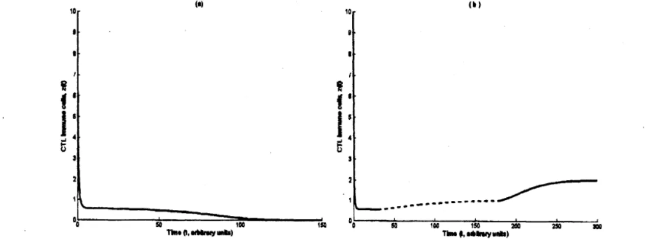
Figure 1: Timeseriesof$z$. The phaseoftreatment is indicatedby dash line. (a)Withouttherapy,

$z(t)$ tendsto zero. (b) After a phase of therapy, which begins at _$t=30$, _{the system will tend to}

inimune control outcome, although the treatment has $l$_)$eer\iota$ stopped at $l=180$

.

Parameter values

are chosen $a8$ follows: $\lambda=1,$$d–0.05.k-0.5,p_{-}--0.3,$_{$c-0.6,\epsilon--0.5_{r}.q--0.2,$}b—-0.2,$\delta--0.3$

.

During therapy, $\delta--\cdot 0.6$

.

An simulation is shown in Fig. 1. The initial values ofthe two trajectories

are

the

same

(20, 10, 10), butthere is

a

phaseof therapy (from $t=30$ to 180) inthe right

one.

Theresults

are

obviously different, i.e., the phase of the therapy leads to

an

immunological control,

instead of the disease outcome in the left

one.

Theoretically, the optImal timing of when therapy should be stopped $and/or$ _restarted

Finally,

we

point out that the bistable behavior as described inthis paper hinges onthe

assumption _that the virus impairs specific immune responses. Therapy

can

therefore shift

the patient from

a

diseaseprogressiontoacontrol outcome. With viruses that donot impair

immunity, there is

no

bistability.

References

[1] Nowak M. A., May R. M., Virus dynamics: Mathematical principles of immunology and

virology, Oxford: Oxford UniversityPress, NewYork, 2000.

[2] Lechner F., WongD. K., DunbarP. R., Chapman R., ChungR. T., Dohrenwend P., Robbins

G., Phillips R., Klenerman P., Walker, B. D., Analysis ofsuccessful immune responses in

persons infected with hepatitis $C$ virus, J. $Exp$

.

Med. 191 (2000) 1499-1512.

[3] Lohr H. F., Krug S., Herr W., Weyer S., Schlaak J., Wolfel T., Gerken G., Meyer zum

Buschenfelde K. H., Quantitative and functional analysis ofcore-speciflc T-helpercell and

CTL activities in acute and chronic hepatitis$B$, Liver 18 (1998) 405-413.

[4] Wodarz D., Christensen J. P., Thomsen A.R., The importance oflyticand

_nonlfiic

immune

responses in viral infection, TRENDS in Immunology 23 (2002) 194-200.

[5] Thieme H. R., Persistence underrelaxed point-dissipativity (with applicationtoan endemic

model), SIAM J. Math.Anal. 24 (1993) 407-435.

[6] Liu X., Takeuchi Y., Spreadofdisease with transport-related infection and entryscreening,

J. Theor. Biol. 242 (2006) 517-528.

[7] KomarovaN.L., Barnes E., KlenermanP., Wodarz D., Boostingimmunity by antiviraldrag

therapy: Asimple relationship among timing, efficacy, and success, Immunology 100 (203)

1855-1860.

[8] Harrer T.,Harrer E., Kalams S.A., ElbeikT., StapransS. I., Feinberg M.B., CaoY.,Ho D.

D., Yilma T., CaliendoA. M., et al., Strongcytotoxic$T$ cell and weak neutralizing antibody

responses in a subset of persons with stable non-progressingHIVtype1 infection, AIDSRes.

Hum. Retroviruses 12 (1996) 585-592.

[9] Lechner F., Gruener N. H., Urbani S., Uggeri J., Santantonio T., Kammer A. R., Cerny

A., Phillips R., Ferrari C., Pape G. R., Klenerman P., $CD8+T$ lymphocyte responses are

inducedduring acute hepatitis $C$ virus infection but are not sustained, Eur. J. Immunol. 30