The Elliptic Representation of the Painleve 6 Equation (Deformation of differential equations and asymptotic analysis)

The

Elliptic Representation

of the

Painleve’

6Equation

Davide Guzzetti –RIMS

1Introduction

We review

our

results, tobe found in [10] [11],

on

theellipticrepresentation of the sixth Painleve’equation

$\frac{d^{2}y}{dx^{2}}=\frac{1}{2}[\frac{1}{y}+\frac{1}{y-1}+\frac{1}{y-x}](\frac{dy}{dx})^{2}-[\frac{1}{x}+\frac{1}{x-1}+\frac{1}{y-x}]\frac{dy}{dx}$

$+ \frac{y(y-1)(y-x)}{x^{2}(x-1)^{2}}[\alpha+\beta\frac{x}{y^{2}}+\gamma\frac{x-1}{(y-1)^{2}}+\delta\frac{x(x-1)}{(y-x)^{2}}]$, (PVI).

Though the elliptic representation of PVI has been known since R.Fuchs [7], in the literature there is

no

general study of its analytic implications. To fill this gaP,

we

studied in [11] the analytic properties

of the solutions in ellipticrepresentationfor $\mathrm{a}11$

(

values of$\alpha$,$\beta,\gamma$,$\delta$ and

we

derived their critical behavior

closeto the singular points $x=0$, 1,$\infty$

.

Moreover,

we

solved the connection problem for generic values

of$\alpha$,$\beta$,$\gamma$,

$\delta$ and in [10] for the special (non-generic)

case

$\beta$$=\gamma=1-2\delta=0$, which is important in 2-D

topological fieldtheory.

The first analytical problem with Painleve’ equations is to determine the critical behavior of the

transcendents

at the critical points$x=0$

,

1,$\infty$

.

Such abehavior must depend

on

twoparameters,which

are

integration constants. The second problem, called connection problem, is to find the relation between

the couples of parameters at different critical points. The method of isomonodromic

deformations

developed in [14] [15]

was

applied to the Painleve’ 6equation in [13], to solve such problems for aclass

of solutions of PVI with generic values of the parameters. The non-generic

case

$\beta=\gamma=1-2\delta=0$ is

studiedin [6] [19] [10] forits applicationstotopological fieldtheory. Studies

on

thecritical behavior

can

be also foundin [25].

Here

we

show that the elliptic representation is avaluable tool to study the critical behavior of

the Painleve’ 6transcendents. In [10] [11]

we

obtained results which include the results of [13] [6]

and extend the class of solutions to which they aPPly. On the other hand,

we

needed to

use

the

isomonodromic deformation theory to solve the connection problem, to be formulated below, for the

elliptic representation.

The elliptic representation

was

introduced by P. Painleve’in [22] and R. Fuchs in [7]. Let

$\mathcal{L}:=x(1-x)\frac{d^{2}}{dx^{2}}+(1-2x)\frac{d}{dx}-\frac{1}{4}$

.

bealinear differential operator and let$\wp(z;\omega_{1}, \omega_{2})$ be theWeierstrass elliptic function of theindependent

variable $z\in \mathrm{P}^{1}$, with half-periods

$\omega_{1}$, $\omega_{2}$

.

Let

us

consider the following independent solutions of the

hyper-geometric equation$\mathcal{L}\omega=0$:

$\{v_{1}(x):=\frac{\pi}{2}F(\frac{1}{2},$ $\frac{1}{2},1;x)$ , $\{v_{2}(x):=i\frac{\pi}{2}F(\frac{1}{2},$$\frac{1}{2},1;1-x)$ ,

where $F$$( \frac{1}{2}, \frac{1}{2},1;x)$ is thestandardnotation forthehyper-geometric function. Here$x$is in the universal

covering of $\mathrm{P}^{1}\backslash \{0,1, \infty\}$,

so

that at this stage

we

do not worry about the choice of branch-cuts. It is

proved in [7] that the Painleve’ 6equation is equivalent to the following differential equation for

anew

function $u(x)$:

$\mathcal{L}(u)=\frac{1}{2x(1-x)}\frac{\partial}{\partial u}\{2\alpha[\wp(\frac{u}{2};\omega_{1},$$\omega_{2})+\frac{1+x}{3}]-2\beta,\frac{x}{\wp(\frac{u}{2}\cdot\omega_{1},(v_{2})+\frac{1+x}{3}}+$

$+2 \gamma\frac{1-x}{\wp(\frac{u}{2}-\omega_{1},\omega_{2})+\frac{x-2}{3}}+(1-2\delta)\frac{x(1-x)}{\wp(\frac{u}{2}-\omega_{1},\omega_{2})+\frac{1-2x}{3}}\}$ (1)

数理解析研究所講究録 1296 巻 2002 年 112-123

The connection to Painleve’ 6is given by the following representation of the transcendents:

$y(x)= \wp(\frac{u(x)}{2};\omega_{1}(x),$$\omega_{2}(x))+\frac{1+x}{3}$.

The algebraic-geometrical properties of the elliptic representations where studied in [18].

Nev-ertheless, the analytic properties of the function $u(x)$

were

not studied, except for the special

case

$\alpha=\beta=\gamma=1-2\delta=0$

.

In this

case

the function $u(x)$ is alinear combination of$\omega_{1}$ and$\omega_{2}$

.

This

case

was

well known to Picard [23], and the critical behavior

was

studied in [19].

In [11],

we

studied the analytic properties of $u(x)$ for any value of $\alpha$,$\beta$,

$\gamma$,

$\delta$

.

As aresult, given

a

Painleve 6equationspecified by achoiceof$\alpha$,$\beta$,$\gamma$,

$\delta$,

we

found the criticalbehavior of its transcendents

belonging to aclass whichcontainsalmostallpossiblesolutionsoftheequation. Themeaning of “almost”

will be clear later. Atranscendent in the class vanishes

as

$x$ (as

as

variable in the universal covering

of$\mathrm{P}^{1}\backslash \{0,1, \infty\})$ approaches acriticalpoint. Nevertheless, along

some

particular paths approaching the

critical point, the transcendent does not vanish: it has oscillatory behavior. Qualitatively speaking,

the oscillations

are

due to the existence of (movable) poles close to the particular paths having

an

accumulation point in thecritical point. In [10] we found analogous results for the special

case

$\beta=\gamma=$

$1-2\delta=0$and $\alpha$

any

complex number

As remarked above,

our

class of solutions include “almost” all transcendents, but there

are some

transcendents which

are

not singed out by

our

method. This is for example the

case

of the Chazy

solutions, whose critical behavior is different from

ours

(see [19]).

2Our results

2.1

Local

Representation

The equation $L(u)=0$ has ageneral solution $u_{0}(x)=2\nu_{1}\omega_{1}(x)+2\nu_{2}\omega_{2}(x)$, $\nu_{1}$,$\nu_{2}\in \mathrm{C}$. We look for a

solution of(1)$\underline{\mathrm{o}\mathrm{f}}$the form $u(x)=2\nu_{1}\omega_{1}(x)+2\nu_{2}\omega_{2}(x)+2v(x)$, where$v(x)$ is aperturbation of$u\circ\cdot$ Let

$\mathrm{C}_{0}:=\mathrm{C}\backslash \{0\}$, $\mathrm{C}_{0}$ the universal covering and let

$0<r<1$

.

Wedefine the domains

$D(r;\nu_{1}, \nu_{2}):=\{x\in\overline{\mathrm{C}_{0}}$ such that $|x|<r$, $| \frac{e^{-i\pi\nu_{1}}}{16^{1-\nu_{2}}}x^{1-\nu_{2}}|<r$,$| \frac{e^{i\pi\nu_{1}}}{16^{\nu_{2}}}x^{\nu\underline{\circ}}|<r\}$ (2)

$D_{0}(r):=\{x\in\overline{\mathrm{C}_{0}}$ such that $|x|<r\}$ (3)

We observe that the translations $\nu_{i}\mapsto\nu_{i}+2N_{i}$, $i=1,2$, $N_{i}\in \mathrm{Z}$ do not change atranscendent in the

elliptic representation

$y(x)= \wp(\nu_{1}\omega_{1}(x)+\nu_{2}\omega_{2}(x)+v(x);\omega_{1}(x),\omega_{2}(x))+\frac{1+x}{3}$

.

This is aconsequence ofthe periodicityofthepfunction. Therefore,

one can

take$0\leq\Re\nu_{i}<2$, $i=1,2$

.

Nevertheless,

we

don’t need to suppose such

arange

explicitly. Only in the

case

$\Im 1\ =0$

we

need to

supposethat $0\leq\nu_{2}<2$. Finally, let us introduce the following expansion:

$v(x; \nu_{1}, \nu_{2}):=\sum_{n\geq 1}a_{n}x^{n}+\sum_{n\geq 0,m\geq 1}b_{nm}x^{n}[e^{-i\pi\nu_{1}}(\frac{x}{16})^{1-\nu_{2}}]^{m}+\sum_{n\geq 0,m\geq 1}c_{nm}x^{n}[e^{i\pi\nu_{1}}(\frac{x}{16})^{\nu_{2}}]^{m}$ (4)

Theorem 1: Let $\nu_{1}$, $\nu_{2}$ be tetto complex numbers.

I) Forany complex $\nu_{1}$, $\nu_{2}$ such that$\Im\nu_{2}\neq 0$ there exist apositive number$r<1$ and

a

transcendent

$\mathrm{y}(\mathrm{x})=\wp(\nu_{1}\omega_{1}(x)+\nu_{2}\omega_{2}(x)+\mathrm{u}(\mathrm{x})\nu_{1},$ $\nu_{2});\omega_{1}(x),\omega_{2}(x))+\frac{1+x}{3}$

such that$v(x;\nu_{1}, \nu_{2})$ is holomorphic in the domain$D(r;\nu_{1}, \nu_{2})$ and it is given by the expansion (4) which

is convergent in$D(r;\nu_{1}, \nu_{2})$

.

The

coefficients

an, $b_{nm}$, $c_{nm}$, $i=1,2$,

are

certain rational

functions of

$\nu_{2}$. Moreover, there exists

a

positive constant $M(\nu_{2})$ such that

$|v(x; \nu_{1}, \nu_{2})|\leq M(\nu_{2})(|x|+|e^{-i\pi\nu_{1}}(\frac{x}{16})^{1-\nu\circ}\sim|+|e^{i\pi\nu_{1}}(\frac{x}{16})^{\nu_{2}}|)$ in $D(r;\nu_{1}, \nu_{2})$ (5)

II) For any complex $\nu_{1}$ and real $\nu_{2}$, with the constraint $0<\nu_{2}<1$ or $1<\nu_{2}<2$, there exists $a$

positive r $<1$ and a transcendent

$\mathrm{y}(\mathrm{x})=\wp(\nu_{1}\omega_{1}(x)+\mathrm{V}2\mathrm{U}2(\mathrm{x})+v(x;\nu_{1}, \nu_{2});\omega_{1}(x),$ $\omega_{2}(x))+\frac{1+x}{3}$,

if

$0<\nu_{2}<1$

or

$\mathrm{y}(\mathrm{x})=\wp(\nu_{1}\omega_{1}(x)+\nu_{2}\omega_{2}(x)+v(x;-\nu_{1},2-\nu_{2});\omega_{1}(x),\omega_{2}(x))+\frac{1+x}{3}$,

if

_{$1<\nu_{2}<2$}

such that$v(x;\nu_{1}, \nu_{2})$ and$v(x;-\nu_{1},2-\nu_{2})$ are holomorphic in$D_{0}(r)$, with convergent expansion (4) and

bound (5) (for $1<\nu_{2}<2$ substitute$\nu_{1}\mapsto-\nu_{1}$, $\nu_{2}\mapsto 2-\nu_{2}$).

Note that in the theorem

$\nu_{2}\neq 0,1$

We stress that in

case

$\mathrm{I}\mathrm{I}$), if

$\nu_{2}$ is greater that

2or

less then 0,

we can

always make atranslation

$\nu_{2}\mapsto\nu_{2}+2N$ to obtain $0<\nu_{2}<2$ (ontheotherhand, $\mathrm{i}\mathrm{f}-2N<\nu_{2}<2-2N$, theformulae of

case

$\mathrm{I}\mathrm{I}$)

hold with the substitution $\nu_{2}\mapsto\nu_{2}+2N$). Note also that $\nu_{1}$ and $\nu_{2}$ Play asymmetric roles.

Observation 1: As aconsequence ofthe theorem, for any $N\in \mathrm{Z}$ and for any complex $\nu_{1}$,$\nu_{2}$ such that

$\propto s\nu_{2}\neq 0$, there exists $rN<1$ and atranscendent $y(x)=\wp(\nu_{1}\omega_{1}(x)+[\nu_{2}+2N]\omega_{2}(x)+v(x;\nu_{1},$$\nu_{2}+$

$2\mathrm{N})$;VO(r),$\omega_{2}(x))+\frac{1+x}{3}$ in $D(r;\nu_{1}, \nu_{2}+2N)$

.

By periodicity of the $\wp-$-function

we

$\mathrm{r}\mathrm{e}$-write the

tran-scendent

as

follows:

$\mathrm{y}(\mathrm{x})=\wp(\nu_{1}\omega_{1}(x)+\mathrm{V}2\mathrm{U}2(\mathrm{x})+\mathrm{v}(\mathrm{x}]\nu_{1}, \nu_{2}+2N);\omega_{1}(x),\omega_{2}(x))+\frac{1+x}{3}$ in $D(r;\nu_{1}, \nu_{2}+2N)$

.

Moreover,

we

showed in [11] that ifatranscendent has the elliptic representation

$y(x)=\wp(\nu_{1}\omega_{1}(x)+\nu_{2}\omega_{2}(x)+v(x;\nu_{1}, \nu_{2});\omega_{1}(x),$$\omega_{2}(x))+\frac{1+x}{3}$

in $D(r, \nu_{1}, \nu_{2})$ for

some

$\nu_{1}$,$\nu_{2}$, $\Im\nu_{2}\neq 0$, then for any integer$N$ there exists $\nu_{1}’$ (depending

on

$\nu_{1}$, $\nu_{2}$ and

$N)$ such that the transcendent has also the representation

$\mathrm{y}(\mathrm{x})=\wp(\nu_{1}’\omega_{1}(x)+\mathrm{V}2\mathrm{U}2(\mathrm{x})+v(x;\nu_{1}, \nu_{2}+2N);\omega_{1}(x),\omega_{2}(x))+\frac{1+x}{3}$

in $\mathrm{V}(\mathrm{r}, \nu_{1}’, \nu_{2}+2N)$

.

$\nu_{1}’$

can

be explicitly computed.

Observation 2: Another

consequence

ofthe theorem is that for any complex $\nu_{1}$,$\nu_{2}$ such that $\Im\nu_{2}\neq 0$

there exists $y(x)= \wp(-\nu_{1}\omega_{1}(x)+[2-\nu_{2}]\omega_{2}(x)+v(x;-\nu_{1},2-\nu_{2});\omega_{1}(x),\omega_{2}(x))+\frac{1+x}{3}$

.

Again

we

use

the fact that the pfunctionisperiodic w.r.t. $2\omega_{2}$ and it is

an

even

function. Therefore the transcendent

becomes

$y(x)=\wp(\nu_{1}\omega_{1}(x)+\nu_{2}\omega_{2}(x)-v(x;-\nu_{1}, 2-\nu_{2});\omega_{1}(x)$,$\omega_{2}(x))+\frac{1+x}{3}$, in $D(r;-\nu_{1},2-\nu_{2})$

Note that the series $-v(x;-\nu_{1},2-\nu_{2})$ is of the form

$\mathrm{I}$_{$a_{n}x^{n}+ \sum_{n\geq 0,m\geq 1}b_{nm}x^{n}[e^{-i\pi\nu_{1}}(\frac{x}{16})^{2-\nu_{2}}]m+\sum_{n\geq 0,m\geq 1}c_{nm}x^{n}[e^{i\pi\nu_{1}}(\frac{x}{16})^{\nu_{2}-1}]m$}

where

we

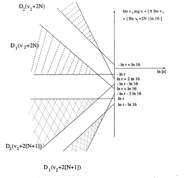
have $\mathrm{r}\mathrm{e}$-named the constants $a_{n}$,$b_{nm}$,$c_{nm}$.

The domain $D(r_{N} ; \nu_{1}, \nu_{2}+2N)$

can

be written

as

follows:

$( \Re\nu_{2}+2N)\ln\frac{|x|}{16}-\pi s\nu_{1}\propto-\ln r_{N}<\propto s\nu_{2}\arg x<$

$<( \Re\nu_{2}-1+2N)\ln\frac{|x|}{16}-\pi s\nu_{1}\propto+\ln r_{N}$, $|x|<r_{N}$

$\mathrm{D}_{1}(\mathrm{v}_{2}+2[\mathrm{N}+1])$

Figure 1: Thedomains$D_{1}(r;\nu_{1}, \nu_{2}+2N):=D(r;\nu_{1}, \nu_{2}+2N)$,$D_{2}(r;\nu_{1}, \nu_{2}+2N):=D(r;-\nu_{1},2-\nu_{2}-2N)$

and $D_{1}(r;\nu_{1}, \nu_{2}+2[N+1])$, $D_{2}(r;\nu_{1}, \nu_{2}+2[N+1])$ for arbitrarily fixed values of $\nu_{1}$, $\mathrm{v}_{2}$, $N$

.

They

are

represented in the plane $(\ln|x|, \Im\nu_{2}\arg x+[\pi\Im\nu_{1}+(\Re\nu_{2}+2N)\ln 16])$.

Therefore the domain $D(rN, -\nu 1,2-\nu 2-2N)$ is

$( \Re\nu_{2}-1+2N)\ln\frac{|x|}{16}-\pi s\nu_{1}\propto-\ln r_{N}<s^{\propto}\nu_{2}\arg x<$

$<( \Re\nu_{2}-2+2N)\ln\frac{|x|}{16}-\pi\Im\nu_{1}+\ln r_{N}$, $|x|<r_{N}$

We

can

draw their picture in the $(\ln|x|, \propto s\nu_{2}\arg x)$ plane

See

figufe 1.

It is remarkable that the ellipticrepresentationallows

us

to

conclude

that the

same

transcendent has

different representations

on

theunion ofthe domains $D(r_{N}, -\nu_{1},2-\nu_{2}-2N)$, $D(r_{N} ; \nu_{1}, \nu_{2}+2N)$

.

The

movable poles ofthe transcendent

are

outside the union.

2.2

Critical Behavior

It is possible to compute the critical behavior for$xarrow \mathrm{O}$ of atranscendent ofTheorem 1. For simplicity,

we

consider $xarrow \mathrm{O}$ along the paths defined below. Let $\propto s\nu_{2}\neq 0$ and $\mathcal{V}\in \mathrm{C}$. We

define

the following

family of paths joining apoint $x0\in D(r;\nu 1, \nu 2)$ to $x=0$

$\arg x=\arg x_{0}+\frac{\Re\nu_{2}-\mathcal{V}}{\propto,s’\nu_{2}}\ln\frac{|x|}{|x_{0}|}$, $0\leq \mathcal{V}\leq 1$ (6)

The paths

are

contained in$D(r;\nu_{1}, \nu_{2})$

.

If|sv2=0any regularpathcontainedin $D_{0}(r)$

can

be

considered

Theorem 2: Let $\nu_{1}$, $\nu_{2}$ be given.

If

$\Im\nu_{2}\neq 0$, the critical behavior

of

the transcendent $y(x)=\wp(\nu_{1}\omega_{1}+\nu_{2}\omega_{2}+v(x;\nu_{1}, \nu_{2});\omega_{1},$$\omega_{2})+$

$(1+x)/3$ when $xarrow \mathrm{O}$ along the path (6) is:

For$0<\mathcal{V}<1$:

$y(x)=- \frac{1}{4}[\frac{e^{i\pi\nu_{1}}}{16^{\nu_{2}-1}}]x^{\nu_{2}}(1+O(|x^{\nu_{2}}|+|x^{1-\nu_{2}}|))$

.

(7)

(8) For$\mathcal{V}=0$:

$\mathrm{y}(\mathrm{x})=[\frac{x}{2}+\sin^{-2}(-i\frac{\nu_{2}}{2}\ln\frac{x}{16}+\frac{\pi\nu_{1}}{2}+\sum_{m\geq 1}c_{0m}[e^{i\pi\nu_{1}}(\frac{x}{16})^{\nu_{2}}]^{m})]$ $(1+O(x))$

.

For$\mathcal{V}=1$:

$y(x)=x \sin^{2}(i\frac{1-\nu_{2}}{2}\ln\frac{x}{16}+\frac{\pi\nu_{1}}{2}+\sum_{m\geq 1}b_{0m}[e^{-i\pi\nu_{1}}(\frac{x}{16})^{1-\nu_{2}}]^{m})(1+O(x))$

.

(9)

For$\nu_{2}$ real

we

have two

cases.

For$0<\nu_{2}<1$, thetranscendent$y(x)=\wp(\nu_{1}\omega_{1}+\nu_{2}\omega_{2}+v(x;\nu_{1}, \nu_{2});\omega_{1},\omega_{2})+$ $(1+x)/3$

defined

in $D_{0}(r)$ has behavior

$\mathrm{y}(\mathrm{x})=-\frac{1}{4}[\frac{e^{i\pi\nu_{1}}}{16^{\nu_{2}-1}}]x^{\nu_{2}}(1+O(|x^{\nu_{2}}|+|x^{1-\nu_{2}}|))$, _{$0<\nu_{2}<1$} (10)

For $1<\nu_{2}<2$, the transcendent$y(x)=\wp(\nu_{1}\omega_{1}+\nu_{2}\omega_{2}+v(x;-\nu_{1},2-\nu_{2});\omega_{1},\omega_{2})+(1+x)/3$

defined

in $D_{0}(r)$ has behavior

$\mathrm{y}(\mathrm{x})=-\frac{1}{4}[\frac{e^{i\pi\nu_{1}}}{16^{\nu_{2}-1}}]-1x^{2-\nu_{2}}(1+O(|x^{2-\nu_{2}}|+|x^{\nu_{2}-1}|))$, _{$1<\nu_{2}<2$} (10)

Note that for$\mathcal{V}=0$the transcendent has oscillatory behavior with

no

limit

as

$xarrow \mathrm{O}$

.

The oscillations

are

due the existence of poles that lie outside the union of the domains of figure 1. They have

an

accumulation point in the critical point $x=0$

.

In [11]

we

showed the existence of such poles in

one

example for $\alpha=\beta=\gamma=1-2\delta=0$

.

2.3

The Critical Points x

$=1$

,

oo

Theorems 1and 2deal with the point $x=0$

.

We

now

turn to the other critical points. Let

us

use

the

notation $\omega_{1}^{(0)}:=\omega_{1}$, $\omega_{2}^{(0)}:=\omega_{2}$; they

are

abasis ofsolutions for the hyper-geometric equation at $x=0$

.

Let us define $\omega_{1}^{(1)}:=\omega_{2}$, $\omega_{2}^{(1)}:=\omega_{1}$: they are abasis of solutions for the hyper-geometric equation at

$x=1$

.

Finally, let $\omega_{1}^{(\infty)}:=\omega_{1}+\omega_{2}$, $\omega_{2}^{(\infty)}:=\omega_{2}$: they

are

abasis ofsolutions for the hyper-geometric

equation at $x=\infty$

.

We construct solutions

$\frac{u(x)}{2}=\nu_{1}^{(1)}\omega_{1}^{(1)}(x)+\nu_{2}^{(1)}\omega_{2}^{(1)}(x)+v^{(1)}(x)$

in aneighborhood of$x=1$, and solutions

$\frac{u(x)}{2}=\nu_{1}^{(\infty)}\omega_{1}^{(\infty)}(x)+\nu_{2}^{(\infty)}\omega_{2}^{(\infty)}(x)+v^{(\infty)}(x)$

inaneighborhood of$x=\infty$. Forthe computationof the criticalbehaviors of$u(x)$

we

need theconnection

formulas for the three bases of solutions ofthe hyper-geometric equation (see [20]). Thus, it is

necessary

to specify branch-cuts in the above definitions. We choose $|\arg x|<\pi$ for$\omega_{1}^{(1)}$, $|\arg(1-x)|<\pi$ for $\omega_{2}^{(1)}$,

$-\pi<\arg x<0$ for $\omega_{1}^{(\infty)}$ and $|\arg x|<\pi$ for$\omega_{2}^{(\infty)}$

.

Once

they

are so

defined, they

are

continued

on

the

universal covering of$\mathrm{P}^{1}\backslash \{0,1, \infty\}$.

We refer to [11] for the analogous ofTheorems 1and 2at $x=1$,$\infty$

.

2.4

Connection

Problem

The elliptic representation allows

us

to obtained detailed information about the critical behavior ofthe

Painleve’ transcendents. On the other hand, the local analysis does not solve the connection problem.

This is the problem of determining the critical behavior of agiven transcendent at $x=0$, $x=1$ and

$x=\infty$. In

our

framework,

we

ask ifatranscendent may have, at the

same

time, three representations

$y(x)= \wp(\nu_{1}^{(0)}\omega_{1}^{(0)}+\nu_{2}^{(0)}\omega_{2}^{(0)}+v^{(0)})+\frac{1+x}{3}$

$= \wp(\nu_{1}^{(1)}\omega_{1}^{(1)}+\nu_{2}^{(1)}\omega_{2}^{(1)}+v^{(1)})+\frac{1+x}{3}$

$= \wp(\nu_{1}^{(\infty)}\omega_{1}^{(\infty)}+\nu_{2}^{(\infty)}\omega_{2}^{(\infty)}+v^{(\infty)})+\frac{1+x}{3}$

.

Moreover,

we

look for formulae which connect the three couples ofparameters $(\nu_{1}^{(0)}, \nu_{2}^{(0)})$, $(\nu_{1}^{(1)}, \nu_{2}^{(1)})$,

$(\nu_{1}^{(\infty)}, \nu_{2}^{(\infty)})$

.

The

connection

problem may be solved using the method of isomonodromic deformations,

as

it

was

firstdone in [13]. ThePVIis the isomonodromydeformation equation ofaFuchsian systemof differential

equations

$\frac{d\mathrm{Y}}{dz}=[\frac{A_{0}(x)}{z}+\frac{A_{x}(x)}{z-x}+\frac{A_{1}(x)}{z-1}]Y$

The 2 $\mathrm{x}2$ matrices _{$A_{i}(x)$} ($i=0$,_$x$,1

are

labels) depend

on

$x$ in such away that the monodromy

of afundamental solution $\mathrm{Y}(z, x)$ does not change for small deformations of $x$

.

They depend

on

the

parameters $\alpha$,$\beta$,

$\gamma$,

$\delta$ ofPVI

as

follows:

$A_{0}(x)+A_{1}(x)+A_{x}(x)=- \frac{1}{2}$ $(\begin{array}{ll}\theta_{\infty} 00 -\theta_{\infty}\end{array})$ , eigenvalues of$A_{i}(x)= \pm\frac{1}{2}\theta_{i}$, $i=0,1$,$x$

$\alpha=\frac{1}{2}(\theta_{\infty}-1)^{2}$, $\beta=-\frac{1}{2}\theta_{0}^{2}$, $\gamma=\frac{1}{2}\theta_{1}^{2}$, $\delta=\frac{1}{2}(1-\theta_{x}^{2})$

In [11]

we

solvedthe connection problem for the elliptic representation for generic values of$\alpha$, $\beta$, $\gamma$,

$\delta$

.

More precisely, by

generic

case we

mean:

$\nu_{2}^{(i)}$,

$\theta_{0}$, $\theta_{x}$, $\theta_{1}$, $\theta_{\infty}\not\in \mathrm{Z}$;

$\frac{\pm 1\pm\nu_{2}^{(i)}\pm\theta_{1}\pm\theta_{\infty}}{2}$

, $\frac{\pm 1\pm\nu_{2}^{(i)}\pm\theta_{0}\pm\theta_{x}}{2}\not\in \mathrm{Z}$

(12)

The signs $\pm \mathrm{v}\mathrm{a}\mathrm{r}\mathrm{y}$ independently. This is atechnical condition which

can

be abandoned (except for

$\nu_{2}^{(i)}\not\in \mathrm{Z})$at the priceofmaking the computations

more

complicated. Forexample, the non-generic

case

$\beta=\gamma=1-2\delta=0$ and at any complex number

was

analyzed in [10] for its relevant applications to

Frobenius manifolds andquantum cohomology.

To summarize the results for the generic case,

we

first observe that the critical behaviors provided

by the elliptic representations along regular paths (except special directions for $\mathcal{V}=0,1$,

see

Theorem

2) at $x=0$, $x=1$ and $x=\infty$ respectively (see [11] for$x=1$,$\infty$)

are

$y(x)=a^{(0)}x^{\nu_{2}^{(0\rangle}}$(1+ higher orders in _$x$), $xarrow \mathrm{O}$ (13)

$y(x)=1-a^{(1)}(1-x)^{\nu_{2}^{(1)}}$_{(1+ higherorders in $(1-x)$),} $xarrow 1$ (14)

$y(x)=a^{(\infty)}x^{1-\nu_{2}^{(\infty)}}$_{( 1+} higherorders in $x^{-1}$), $xarrow\infty$ (15)

and the parameters $\nu_{1}^{(i)}$

are

given by

$e^{i\pi\nu_{1}^{(\mathrm{O})}}=-4a^{(0)}16^{\nu_{\mathrm{Q}}^{(0)}-1}\sim$

, $e^{-i\pi\nu_{1}^{(1)}}=-4a^{(1)}16^{\nu_{2}^{(1)}-1}$

, $e^{i\pi\nu_{1}^{(\propto)}}=-4a^{(\infty)}16^{\nu_{2}^{(\propto)}-1}$

If$\nu_{2}^{(i)}$ is real, the behavior is

as

above when $0<\nu_{2}^{(i)}<1$

.

Otherwise, when $1<\nu_{2}^{(i)}<2$ it is:

$\mathrm{y}(\mathrm{x})=a^{(0)}x^{2-\nu_{\underline{\mathrm{Q}}}^{(())}}$(1+ higherorders in

$x$), $xarrow \mathrm{O}$ (1)

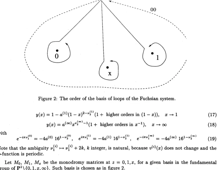
Figure 2: The order of the basisof loops of the Fuchsian system.

$y(x)=1-a^{(1)}(1-x)^{2-\nu_{2}^{(1)}}$₍$1+\mathrm{h}\mathrm{i}\mathrm{g}\mathrm{h}\mathrm{e}\mathrm{r}$ orders in $(1-x)$), $xarrow 1$ (17)

$y(x)=a^{(\infty)}x^{\nu_{2}^{(\infty)}-1}$($1+\mathrm{h}\mathrm{i}\mathrm{g}\mathrm{h}\mathrm{e}\mathrm{r}$ orders in $x^{-1}$), _{$xarrow\infty$} (18)

with

$e^{-i\pi\nu_{1}^{(\mathrm{O})}}=-4a^{(0)}16^{1-\nu_{2}^{(\mathrm{O})}}$ $e^{i\pi\nu_{1}^{(1)}}=-4a^{(1)}16^{1-\nu_{2}^{(1)}}$ $e^{-i\pi\nu_{1}^{(\infty)}}=-4a^{(\infty)}16^{1-\nu_{2}^{(\infty)}}$

(19)

Note that theambiguity $\nu_{1}^{(i)}\mapsto\nu_{1}^{(i)}+2k$, $k$ integer, is natural, because $v^{(i)}(x)$ does not changeand the

$\wp$-function is periodic.

Let $M_{0}$, $M_{1}$, $M_{x}$ be the monodromy matrices at $z=0,1$ ,$x$, for agiven basis in the

fundamental

group

of$\mathrm{P}^{1}\backslash \{0,1, x, \infty\}$

.

Such basis is chosen

as

infigure 2.

If

$\theta_{0}$, $\theta_{x}$, $\theta_{1}$, $\theta_{\infty}\not\in \mathrm{Z}$

thereis

aone

to

one

correspondence between agiven choiceofmonodromy data 00,$\theta_{x}$, $\theta_{1}$, $\theta_{\infty}$, $tr(M0Mx)$,

$\mathrm{t}\mathrm{r}(M_{0}M_{1})$, $\mathrm{t}\mathrm{r}(M_{1}M_{x})$ and atranscendent $y(x)$ (see[13] [6], [10]). Namely:

$\mathrm{y}(\mathrm{x})=y(x;\theta_{0}, \theta_{x}, \theta_{1}, \theta_{\infty}, \mathrm{t}\mathrm{r}(M_{0}M_{x}), \mathrm{t}\mathrm{r}(M_{0}M_{1}), \mathrm{t}\mathrm{r}(M_{1}M_{x}))$ (20)

We proved that such atranscendent has elliptic representations at $x=0,1$,$\infty$, provided that (12) is

satisfied. The three sets ofparameters $(\nu_{1}^{(i)}, \nu_{2}^{(i)})$, $i=0,1$,$\infty$

are

functions of the monodromy data $\theta_{0}$,

$\theta_{x}$, $\theta_{1}$, $\theta_{\infty}$, $tr(M0Mx)$, $\mathrm{t}\mathrm{r}(M_{0}M_{1})$, $\mathrm{t}\mathrm{r}(M_{1}M_{x})$

.

Namely,

we

showed that

2$\cos(\pi\nu_{2}^{(0)})=-\mathrm{t}\mathrm{r}(M_{0}M_{x})$, 2$\cos(\pi\nu_{2}^{(1)})=-\mathrm{t}\mathrm{r}(M_{1}M_{x})$, 2$\cos(\pi\nu_{2}^{(\infty)})=-\mathrm{t}\mathrm{r}(M_{0}\mathrm{J}/I_{1})$ (21) $a^{(i)}=a^{(i)}(\nu_{2}^{(i)} ; \theta_{0}, \theta_{x}, \theta_{1}, \theta_{\infty}, \mathrm{t}\mathrm{r}(M_{0}M_{x}), \mathrm{t}\mathrm{r}(M_{0}M_{1}), \mathrm{t}\mathrm{r}(M_{1}M_{x}))$ , $i=0,1$,

oo

(22)

The formulas of $a^{(i)}$

are

quite long,

so we

do not write them here. They depend

on

the monodromy

datathroughrational, trigonometricand$\Gamma$-functions. In particular,$\nu_{2}^{(i)}$ enters explicitly. Theprocedure

for computing such formulae is given in the Appendix of [11]. We note that the condition $\nu_{2}^{(i)}\not\in \mathrm{z}$ is

equivalent to $\mathrm{t}\mathrm{r}(MiMj)\neq\pm 2$.

Conversely, we proved that atranscendent $y(x)$ _{given by its elliptic representation, under the}

condi-tionsof Theorem 1(and Theorem 3of [11]), is atranscendent (20). This follows from the consideration

that the couple$(\nu_{1}^{(i)}, \nu_{2}^{(i)})$ isgiven at thecritical point $x=i$, and $\theta_{0}$, $\theta_{x}$, $\theta_{1}$, $\theta_{\infty}$

are

fixed by the equation

PVI

we are

considering. From these data

we

can

compute $\mathrm{t}\mathrm{r}(\Lambda f_{0}\mathrm{J}/f_{x})$, $\mathrm{t}\mathrm{r}(M_{1}M_{x})$, $\mathrm{t}\mathrm{r}(\Lambda f_{0}M_{1})$. One of

the traces is -2$\cos(\pi\nu_{2}^{(i)})$, the others depend

on

$\nu_{1}^{(i)}$,$\nu_{2}^{(i)}$,

$\theta_{0}$, $\theta_{x}$, $\theta_{1}$, $\theta_{\infty}$ through rational, trigonometric

and $\Gamma$-functions. The formulae

are

rather long,

so

we

refer the reader to the Appendix of [11]. In this

way the transcendent (20) is obtained. From the monodromy data

we

compute the couples $(\nu_{1}^{(j)}, \nu_{2}^{(j)})$

at the other two critical points and we get the the elliptic representation ofthe initial transcendent at the other critical points. Therefore, the connection problem is solved.

Note that if

we

startfrom the elliptic representation at

one

critical point, sayfor example$x=0$, then

$\nu_{1}^{(0)}$,$\nu_{2}^{(0)}$

are

given. Asexplained above,

we can

computethe monodromy data andfromthem

we

compute $\nu_{2}^{(j)}$ and $a^{(j)}$ (then $\nu_{1}^{(j)}$) at the other two critical points. As already observed, the ambiguity $\nu_{1}^{(g)}\mapsto$

$\nu_{1}^{(j)}+2k$ ($k$ integer) does not change the elliptic representation. On the other hand, the ambiguities

$\nu_{2}^{(j)}\mapsto\nu_{2}^{(j)}+2N$ ($N$ integer), $\nu_{2}^{(j)}\mapsto-\nu_{2}^{(j)}$ and the ambiguity in the choice $0\leq\Re\nu_{2}^{(j)}\leq 1$

or

$1\leq$

$\Re\nu_{2}^{(j)}\leq 2$, which results from the cosines in (21), is due to the fact that the

same

transcendent has

different

elliptic representations in different domains (the choice of $\nu_{2}^{(j)}$ determines the representation

and the domain!).

To summarize the results,

we

say that :

Inthe generic

case

(12) there is $a$one-tO-One correspondence between monodromy data and

transcen-dents (20).

_If

$tr(M_{i}M_{j})\neq\pm 2$ they have elliptic representation whose parameters $(\nu_{1}^{(i)}, \nu_{2}^{(i)})$

are

given

by the

_formulae

(21), (22), (19). Conversely,

a

transcendent whose elliptic representation

_satisfies

the

conditions

_of

Theorem 1(and Theorem

_3of

[11]) is a transcendet (20). The connection between its three

pairs $(\nu_{1}^{(i)}, \nu_{2}^{(i)})$ is explained above. This solves the connection problem.

To conclude the discussion of thegeneric case,

some

commentsabout

our

extension of previous known

results

are

in order. The critical behavior for aclass ofsolutions to thePainleve’ 6equation

was

found

by Jimbo in [13] for generic values of$\alpha$, $\beta$, $\gamma\delta$. Atranscendent in this class has behavior:

$y(x)=a^{(0)}x^{1-\sigma^{(0)}}(1+O(|x|^{\delta}))$, $xarrow \mathrm{O}$, (23)

$y(x)=1-a^{(1)}(1-x)^{1-\sigma^{(1)}}(1\mathrm{t}O(|1-x|^{\delta}))$, $xarrow 1$, (24)

$\mathrm{y}(\mathrm{x})=a^{(\infty)}x^{-\sigma^{(\infty)}}(1+O(|x|^{-\delta}))$, $xarrow\infty$, (23)

where $\delta$is asmall positive number, $a^{(i)}$ and $\sigma^{(i)}$

are

complex numbers such that $a^{(i)}\neq 0$ and

$0\leq\Re\sigma^{(i)}<1$

.

(26)

We remark that $x$convergestothe critical points inside a sectorwith vertex

on

the corresponding critical

point. Theconnection problem, i.e. the problemoffinding the relationamongthe three pairs $(\sigma^{(i)}, a^{(i)})$,

$i=0,1$,$\infty$,

was

solvedin [13] for the above class of transcendentsusing the isomonodromy deformations

theory. Actually, atranscendent in the class above coincides with atranscendent (20). In particular

2$\cos(\pi\sigma^{(0)})=\mathrm{t}\mathrm{r}(M_{0}M_{x})$, 2$\cos(\pi\sigma^{(1)})=\mathrm{t}\mathrm{r}(M_{1}M_{x})$, 2$\cos(\pi\sigma^{(\infty)})=\mathrm{t}\mathrm{r}(M_{0}M_{1})$ (27)

and

$a^{(i)}=a^{(i)}(\sigma^{(i)} ; \theta_{0}, \theta_{x}, \theta_{1}, \theta_{\infty}, tr(MiMx), \mathrm{t}\mathrm{r}(M_{0}M_{1}), \mathrm{t}\mathrm{r}(M_{1}M_{x}))$, $i=0,1$,$\infty$

For the formulas of$a^{(i)}$

we

refer to [13]. The monodromy data

are

restricted by the following condition,

equivalent to (26):

$|\mathrm{t}\mathrm{r}(M_{i}M_{j})|\leq 2$, $\Re\{\mathrm{t}\mathrm{r}(MiMj)\}\neq-2$ (28)

As explained above, we have shown that the transcendents (20) have elliptic representation.

There-fore, Jimbo’s transcendents

are

included in

our

class of transcendents obtained by the elliptic

represen-tation. Observethat the behaviors (23)-(25)

are

included in the behaviors (13)-(15) with $\sigma^{(i)}=1-\nu_{2}^{(i)}$

(and (16)-(18) with$\sigma^{(i)}=\nu_{2}^{(i)}-1$). We proved in [11] that the condition (26) isextended toany$\sigma^{(i)}\in \mathrm{c}$

such that$\sigma^{(i)}\not\in(-\infty, 0]\cup[1, +\infty)$ (as

we

must expect, if

we

observe that $\nu_{2}^{(i)}\not\in(-\infty, 0]\cup\{1\}\cup[2, +\infty)$

and that (27) defines $\sigma^{(i)}$ up to $\sigma^{(i)}\mapsto\pm\sigma^{(i)}+2n$, _$n$ integer). Therefore

we

have solved the connection

problem for any complex value of $\mathrm{t}\mathrm{r}(M_{i}M_{j})$ with the only

constraint

$\mathrm{t}\mathrm{r}(M_{i}M_{j})\neq\pm 2$. This condition

extends (28).

To be

more

precise, the condition $\nu_{2}^{(i)}\neq 1$ is equivalent to $\mathrm{t}\mathrm{r}(M_{0}\Lambda f_{x})\neq 2$ at $x=0$; to $\mathrm{t}\mathrm{r}(M_{1}M_{x})\neq 2$

at $x=1$;to $\mathrm{t}\mathrm{r}(hf_{0}M_{1})\neq 2$ at $x=\infty$. Nevertheless, in the

case

$\mathrm{t}\mathrm{r}(NI_{i}NI_{j})=2$ the critical behavior

and the solution of the connection problem

were

achieved by Jimbo. Unfortunately, the condition

$\nu_{2}^{(i)}\neq 1$ which

we

had to impose to study the elliptic representation (except for non-generic

case

$\mathrm{s}$ like

$\beta=\gamma=1-2\delta=0)$ does not allow

us

to know the analytic properties and the critical behavior of the

elliptic representation in this case. We expect that the properties of $u(x)$ are such to exactly produce

the critical behavior found by Jimbo for $\mathrm{t}\mathrm{r}(MiMj)=2$, but

we

still have to

cover

this

case.

The condition $\nu_{2}^{(i)}\neq 0$ (and 2), implies that we

can

not give the critical behaviors

(and the elliptic

representation) of (20) at $x=0$ for $\mathrm{t}\mathrm{r}(M_{0}M_{x})=-2$;at $x=1$ for $\mathrm{t}\mathrm{r}(M_{1}M_{x})=-2$;at $x=\mathrm{o}\mathrm{o}$ for

$\mathrm{t}\mathrm{r}(M_{0}M_{1})=-2$. Toour knowledge, these

cases

have not yet been studied in the literature.

To conclude, the results of [13] together with

our

extension provide the critical behaviors and the

solution ofthe connection problem for thetranscendents (20) in the generic

case

for

any

value of$\mathrm{t}\mathrm{r}(M_{i}M_{j})\neq-2$

which corresponds to exponents

$\sigma^{(i)}\in \mathrm{C}$ such that _{$\sigma^{(i)}\not\in(-\infty, 0)\cup[1, +\infty)$}

.

We turn

now

to the special

case

$\beta=\gamma=1-2\delta=0$, important for its applications _{to topological}

filed theory, Frobenius manifolds [4] and quantum cohomology [17] [12]. This

case

is fully studied in

[10]. We

can

give arepresentation of$u(x)$ in adomain whichis wider than_thegeneric

case.

_{Namely, at}

$x=0$, the domain is

$D(rj\nu_{1}, \nu_{2}):=\{x\in\tilde{\mathrm{C}}\circ||x|<r$, $|e^{-i\pi\nu_{1}}( \frac{x}{16})^{2-\nu_{2}}|<r$, $|e^{i\pi\nu_{1}}( \frac{x}{16})^{\nu_{2}}|<r\}$

In this domain $v(x)$ is holomorphic with convergent expansion

$v(x)= \sum_{n\geq 1}a_{n}x^{n}+\sum_{n\geq 0,m\geq 1}b_{nm}x^{n}[e^{-i\pi\nu_{1}}(\frac{x}{16})^{2-\nu_{2}}]^{m}+\sum_{n\geq 0,m\geq 1}c_{nm}x^{n}[e^{i\pi\nu_{1}}(\frac{x}{16})^{\nu_{2}}]^{m}$

If$\nu_{2}$ is real, thevalue$\nu_{2}=1$ is

now

allowed, namely, theconstraint is $\iota \mathrm{g}$ $\not\in(-\infty, 0]\cup[2, +\infty)$

.

Therefore,

by periodicity ofthe pfunction

we can

assume

$0\leq\Re\nu_{2}<2$, $\nu_{2}\neq 0$

.

Asimilar result holds at $x=1$

and $x=\infty$

.

According to [6],

we

define $2-x_{0}^{2}:=\mathrm{t}\mathrm{r}$ $M_{0}M_{x}$, $2-x_{1}^{2}:=\mathrm{t}\mathrm{r}$ MOMX, $2-x_{\infty}^{2}:=\mathrm{t}\mathrm{r}$ $M_{0}M_{1}$

.

There

is

aone

to

one

correspondence between triples $(x_{0}, x_{1}, x_{\infty})$ (defined uPto the change of two signs) and

Painleve’ transcendents, provided that at most

one

$x_{i}$ is

zero

and not all the $x_{i}$

are

+2 at the

same

time. Therefore

we

write $y(x)=y(x;x0, x_{1}, x_{\infty})$. We show that

one

such transcendent has elliptic

representations (half-periods

are

understood)

$y(x;x_{0}, x_{1}, x_{\infty})= \wp(\nu_{1}^{(0)}\omega_{1}^{(0)}(x)+\nu_{2}^{(0)}\omega_{2}^{(0)}(x)+v^{(0)}(x;\nu_{1}^{(0)}, \nu_{2}^{(0)}))+\frac{1+x}{3}$

$= \wp(\nu_{1}^{(1)}\omega_{1}^{(1)}(x)+\nu_{2}^{(1)}\omega_{2}^{(1)}(x)+v^{(1)}(x;\nu_{1}^{(1)}, \nu_{2}^{(1)}))+\frac{1+x}{3}$ (29)

$= \wp(\nu_{1}^{(\infty)}\omega_{1}^{(\infty)}(x)+\nu_{2}^{(\infty)}\omega_{2}^{(\infty)}(x)+v^{(\infty)}(x;\nu_{1}^{(\infty)}, \nu_{2}^{(\infty)}))+\frac{1+x}{3}$ (30)

The parameters $\nu_{2}^{(i)}$

are

obtained from

$\cos\pi\nu_{2}^{\langle i)}=\frac{x_{i}^{2}}{2}-1$, $0\leq\Re\nu_{2}^{(i)}\leq 1$, $\nu_{2}^{(i)}\neq 0$, $i=0,1$,

oo

Note that the condition $x_{i}\neq\pm 2$, $i=0,1$,$\infty$, corresponds to $\nu_{2}^{(i)}\neq 0$

.

The parameter $\nu_{1}^{(0)}$ is obtained

by the formul

$e^{i\pi\nu_{1}^{(0)}}=- \frac{i\Gamma^{4}(1--\nu_{2}^{(0)}=)}{2\sin(\pi\nu_{2}^{(0)})\Gamma^{2}(\frac{3}{2}-\mu-\underline{\nu}_{2}^{(0)}=)\Gamma^{2}(\frac{1}{2}+\mu-\underline{\nu}_{2}^{(\mathrm{O})}arrow)}[2(1-e^{i\pi\nu_{\underline{\mathrm{Q}}}^{(()\rangle}})-$

$-f(x_{0}, x_{1}, x_{\infty})(x_{\infty}^{2}-e^{i\pi\nu_{2}^{(0)}}x_{1}^{2})]\mathrm{u}(\mathrm{x})x_{1},$$x_{\infty})$

$f(x_{0}, x_{1}, x_{\infty}):= \frac{4-x_{0}^{2}}{x_{1}^{2}+x_{\infty}^{2}-x_{0}x_{1}x_{\infty}}$, $\alpha=\frac{(2\mu-1)^{2}}{2}$

Moreover,$\exp\{-i\pi\nu_{1}^{(1)}\}$,$\exp\{i\pi\nu_{1}^{(\infty)}\}$

are

given byananalogous formula with the substitutions$(x_{0},$$x_{1}$,$x_{\mathrm{o}}$

$(x_{1}, x_{0}, x_{0}x_{1}-x_{\infty})$, $\nu_{2}^{(0)}\mapsto\nu_{2}^{(1)}$ and $(x_{0}, x_{1}, x_{\infty})\mapsto(x_{\infty}, -x_{1}, x_{0}-x_{1}x_{\infty})$, $\nu_{2}^{(0)}\mapsto\nu_{2}^{(\infty)}$ respectively.

The most general choice of $\nu_{2}$ is $0\leq\Re\nu_{2}<2$

.

This corresponds to the fact that the transcendent

$y(x;x_{0}, x_{1}, x_{\infty})$ also has three representations

$y(x;x_{0}, x_{1}, x_{\infty})= \wp(\tilde{\nu}_{1}^{(0)}\omega_{1}^{(0)}(x)+\tilde{\nu}_{2}^{(0)}\omega_{2}^{(0)}(x)+v^{(0)}(x;\tilde{\nu}_{1}^{(0)},\tilde{\nu}_{2}^{(0)}))+\frac{1+x}{3}$

$= \wp(\tilde{\nu}_{1}^{(1)}\omega_{1}^{(1)}(x)+\tilde{\nu}_{2}^{(1)}\omega_{2}^{(1)}(x)+v^{(1)}(x_{j}\tilde{\nu}_{1}^{(1)},\tilde{\nu}_{2}^{(1)}))+\frac{1+x}{3}$

$= \wp(\tilde{\nu}_{1}^{(\infty)}\omega_{1}^{(\infty)}(x)+\tilde{\nu}_{2}^{(\infty)}\omega_{2}^{(\infty)}(x)+v^{(\infty)}(x;\tilde{\nu}_{1}^{(\infty)},\tilde{\nu}_{2}^{(\infty)}))+\frac{1+x}{3}$

where

$\cos\pi\tilde{\nu}_{2}^{(i)}=\frac{x_{i}^{2}}{2}-1$, $1\leq\Re\nu_{2}^{(i)}<2$, _$i=0,1$,

oo

The parameter $\tilde{\nu}_{1}^{(0)}$ is obtained bythe formula

$e^{-i\pi\overline{\nu}_{1}^{(0)}}= \frac{i\Gamma^{4}(-\overline{\nu}_{2}^{(0)}=)}{2\sin(\pi\tilde{\nu}_{2}^{(0)})\Gamma^{2}(\frac{1}{2}-\mu+=)\underline{\overline{\nu}}_{2}^{(0)}\Gamma^{2}(-\frac{1}{2}+\mu+p\nu_{2})}[2(1-e^{-i\pi\overline{\nu}_{2}^{(0)}})-$

$-f(x_{0},x_{1}, x_{\infty})(x_{\infty}^{2}-e^{-i\pi\tilde{\nu}_{2}^{(0)}}x_{1}^{2})]$ p{ 0’$x_{1},$$x_{\infty}$).

$\exp\{i\pi\tilde{\nu}_{1}^{(1)}\}$, $\exp\{-i\pi\tilde{\nu}_{1}^{(\infty)}\}$

are

given by an analogous formula with the substitutions $(x_{0}, x_{1}, x_{\infty})\mapsto$

(31)$x_{0},$$x_{0}x_{1}-x_{\infty}),\tilde{\nu}_{2}^{(0)}\mapsto\tilde{\nu}_{2}^{(1)}$ and $(x_{0}, x_{1}, x_{\infty})\mapsto(x_{\infty}, -x_{1}, x_{0}-x_{1}x_{\infty}),\tilde{\nu}_{2}^{(0)}\mapsto\tilde{\nu}_{2}^{(\infty)}$ respectively.

Theformulae above have limits for $\nu_{2}=1,1\pm 2\mu+2m$, $m$ integer. They

are

listed in [10] and [11].

Conversely, atranscendent

$\mathrm{y}(\mathrm{x})=\wp(\nu_{1}\omega_{1}^{(0)}(x)+\nu_{2}\omega_{2}^{(0)}(x)+v^{(0)}(x;\nu_{1}, \nu_{2}))+\frac{1+x}{3}$, at $x=0$ (31)

coincides with $y(x;x_{0}, x_{1}, x_{\infty})$, with thefollowing monodromy data.

If$0\leq\Re\nu_{2}\leq 1$:

$x_{0}=2 \cos(\frac{\pi}{2}\nu_{2})$

$x_{1}=[ \frac{4^{-\nu_{2}}2e^{i\frac{\pi}{2}\nu_{1}}}{f(\nu_{2},\mu)G(\nu_{2},\mu)}+\frac{G(\nu_{2},\mu)}{4^{-\nu_{2}}2e^{i\frac{\pi}{2}\nu_{1}}}]$

$x_{\infty}=[ \frac{4^{-\nu_{2}}2e^{i\frac{\pi}{2}(\nu_{1}-\nu_{2})}}{f(\nu_{2},\mu)G(\nu_{2},\mu)}+\frac{G(\nu_{2},\mu)}{4^{-\nu_{2}}2e^{i\frac{\pi}{2}(\nu_{1}-\nu_{2})}}]$

where

$f( \nu_{2}, \mu)=-\frac{2\sin^{2}(\frac{\pi}{2}\nu_{2})}{\cos(\pi\nu_{2})+\cos(2\pi\mu)}$, $G( \nu_{2}, \mu)=4^{-\nu_{2}}2\frac{\Gamma(1--\nu_{2}A)^{2}}{\Gamma(\frac{3}{2}-\mu--\nu_{2}A)\Gamma(\frac{1}{2}+\mu-\frac{\nu\circ}{2})}$

If $1\leq\Re\nu_{2}<2$:

$x_{0}=2 \cos(\frac{\pi}{2}\nu_{2})$

$x_{1}=[ \frac{e^{-i\frac{\pi}{2}\nu_{1}}}{4^{1-\nu_{2}}2f(\nu_{2},\mu)G_{1}(\nu_{2}./\iota)}+\frac{4^{1-\nu_{2}}2G_{1}(\nu_{2},\mu)}{e^{-i\frac{\pi}{?}\nu_{1}}}]$

$x_{\infty}=[ \frac{e^{i\frac{\pi}{\sim 9}(\nu_{2}-\nu_{1})}}{41-\nu\circ\sim 2f(\nu_{2},\mu)G_{1}(\nu_{2},\mu)}+\frac{4^{1-\nu_{2}}2G_{1}(\nu_{2},\mu)}{e^{i\frac{\pi}{\sim \mathrm{Q}}(\nu\circ-\nu_{1})}\sim}]$

where

$G_{1}( \nu_{2}, \mu)=\frac{1}{4^{1-\nu_{2}}2}\frac{\Gamma(^{\underline{\nu_{2}}}\mathrm{z})^{2}}{\Gamma(\frac{1}{2}-\mu+p\nu_{2})\Gamma(-\frac{1}{2}+\mu+\frac{\nu\circ}{2})}$

After computing the monodromy data,

we can

write the elliptic representations of $y(x;x_{0}, x_{1}, x_{\infty})$ at

$x=1$ and$x=\infty$, namely (29), (30).

Since

they

are

the elliptic representations at$x=1$, $x=\infty$ of(31),

we

havesolved the connection problem for (31).

Weobserved that there is

aone

to

one

correspondence between Painleve’ transcendents and triples of

monodromydata$(x_{0}, x_{1}, x_{\infty})$, defined uP tothe change of two signs, satisfying$x_{i}\neq\pm 2$, $i=0,1$,$\infty$, i.e.

$\nu_{2}^{(i)}\neq 0$ (and 2), and at most

one

_{$x_{i}=0$}

.

The

cases

when these conditions

are

not satisfied

are

studied

in [19]. However,if$x_{i}=\pm 2$ (namely the$\mathrm{t}\mathrm{r}\mathrm{a}\mathrm{c}\mathrm{e}\mathrm{i}\mathrm{s}-2$) the problemoffindingthe critical behavior at the

corresponding criticalpoint $x=i$ is still open (except when all the three $x_{i}$

are

82: in this

case

there is

aone-parameter class of solutions called Chazy solutions in [19]$)$. We conclude that the results of

our

papers [10] [11] plus the resultsof[19]

cover

all the possible transcendents, except thespecial

case

when

one or

two$x_{i}$

are

82.

Finally,

we

expect that in all non-generic

cases

we can

solve theconnection problem and

express

the

parameters$\nu_{1}$, $\nu_{2}$in termsof monodromy data. From theconceptualpointof view nothing should change

with respect to [13] [6] [10] [11]; but the technical details

may

require along time for computations.

Acknowledgments: Iam grateful to B.Dubrovin for many discussions and advice. Iwould like to thank

A.Bolibruch, A.Its, M. Jimbo, M.Mazzocco, S.Shimomura for fruitful discussions which helped

me

to

write [10] [11]. Theauthoris supported by afellowship ofthe Japan Society forthePromotionof

Science

(JSPS).

References

[1] DijkgraafR.,Verlinde E., Verlinde H.: Topological Strings in d $<1$

.

Nucl. Phys B, 352, (1991),

59-86.

[2] B.Dubrovin: Integrable Systemsin Topological Field Theory. Nucl. Phys B, 379, (1992),

627-689.

[3] B.Dubrovin: Geometrry

of

2D topological

_field

theories. Lecture Notes in Math, 1620, (1996),

120-348.

[4] B.Dubrovin: Painleve trascendents in tw0-dimensional topological field theory. The Painleve

Prop-erty, One Century later, R.Conte, Springer 1999.

[5] B.Dubrovin: Differential geometry

on

thespaceof orbits ofaCoxeter group. Surv.

_Differ.

Geom.,

IV, 181-211, Int. Press, Boston, MA, (1998).

[6] B.Dubrovin-M.Mazzocco: MonodromyofCertainPainlev\’e-VItrascendentsandReflection Groups.

Invent, math., 141, (2000),

55-147.

[7] Fuchs R.: Uber lineare homogene Differentialgleichungen zweiter Ordnung mit drei im Endlichen

gelegenen wesentlich singularen Stellen. Mathematische Annalen LXIII, (1907),

301-321

[8] GambierB.: Surdes EquationsDifferentiellesdusecond Ordreet duPremier Degre’dontl’Int\’egrale

est \‘a_{Points Critiques} Fixes. Acta Math., 33, (1910), 1-55

[9] Guzzetti D: Stokes matrices and monodromy for the quantum cohomology of projective spaces.

Comm.Math.Phys. 207, (1999),

341-383.

[10]

Guzzetti D:On

the Critical Behavior, the

Connection

Problem and the EllipticRepresentation of

aPainleve 6Equation . Mathematical Physics, Analysis and Geometry, 4, (2001), 293-377

[11] Guzzetti D: The Elliptic Representation of the General Painleve’ 6Equation. Communications in

Pure and Applied Mathematics, Vol LV (2002).

[12] Guzzetti D:Inverse Problem and MonodromyData for 3-dimensional Frobenius Manifolds .

Afath-ematical Physics, Analysis and Geometry, 4, (2001), 254-291.

[13] M.Jimbo: Monodromy Problem and the Boundary Condition for Some Painleve’ Trascendents.

Publ. RIMS, Kyoto Univ.,18 (1982),

1137-1161.

[14] MJimbo, T.Miwa, K.Ueno: Monodromy PreservingDeformations ofLinear Ordinary Differential

Equations with Rational Coefficients (I). Physica, D2, (1981),

306

[15] MJimbo, T.Miwa :Monodromy Preserving Deformations of Linear Ordinary Differential

Equa-tions with Rational Coefficients (II). Physica , D2, (1981),

407-448

[16] MJimbo, T.Miwa :Monodromy Preserving Deformations of Linear Ordinary Differential

Equa-tions withRational Coefficients (III). Physica, D4, (1981), 26

[17] Kontsevich M., Manin Y.I. : Gromov-Witten classes, Quantum Cohomology and Enumerative

Geometry. Comm.Math. Phys, 164, (1994),

525-562

[18] Manin V.I. : Sixth Painleve Equation, Universal Elliptic Curve, and Mirror of$\mathrm{P}^{2}$

.

Geometry

of

differential

equations, Amer. Math. Soc. Transl. Ser 2, 186, Amer. Math. Soc, Providence, RI,

(1998), 131-151

[19] M.Mazzocco: Picard and Chazy Solutions to the Painleve VI Equation. Math. Ann., 321, no.1,

(2001), 157-195.

[20] N.E.Norlund: The

Loga-ritmic Solutions of the Hypergeometric Equation. Mat.Fys.Skr.Dan.Vid.Selsk., 2, (1963),

no.

5,

1-58

[21] Painleve P.:

Sur

lesEquationsDifferentielles du Second Ordreetd’Ordre Superieur,dontlTntegrale

G\’en\’erale est Uniforme. Acta Math, 25, (1900),

1-86

[22] Painleve P.: Sur les Equations differentielles du second ordre \‘a points critiques fixes. CRAS 143

(1906) 1111-1117.

[23] Picard, E.: Memoire

sur

la Theorie des functions algebriques de deux variables. Journal de

Liou-ville, 5, (1889), 135- 319

[24] M.Sato, T.Miwa, M.Jimbo: Holonomic Quantum Fields. II -The Riemann-Hilbert Problem -.

Publ. RIMS. Kyioto. Univ, 15, (1979), 201-278.

[25] S.Shimomura: Painleve Trascendents in the Neighbourhood of Fixed Singular Points.

Funk-cial. Ekvac., 25, (1982),

163-184.

Series Expansions of Painleve Trascendents in theNeighbourhood ofaFixedSingular Point.

Punk-cial.Ekvac.,25, (1982),

185-197.

Supplement to “Series Expansions ofPainleve Trascendents in theNeighbourhood of aFixed

Sin-gular Point”. Funkcial.Ekvac.,25, (1982),

363-371.

AFamily ofSolutionsofaNonlinear OrdinaryDifferntial Equationand its Application to Painleve

Equations (III), (V), (VI). J. Math. Soc. Japan, 39, (1987),

649-662.

[26] Witten E.: On the Structure ofthe TopologicalPhase ofTwo Dimensional Gravity. Nucl. PhysB,

340, (1990), 281-332