Gradient estimates for mean curvature flow with Neumann boundary conditions (Theory of evolution equations and applications to nonlinear problems)

全文

(1)35. 数理解析研究所講究録第2066巻 2018年 35-45. Gradient estimates for mean curvature flow. with Neumann boundary conditions Masashi Mizuno and Keisuke Takasao. 1. Mean curvature flow. We consider the following parabolic partial differential equation:. \{. (MCF). \displaystyle\frac{\partial_{t}u{\sqrt{1+|du|^{2} =\mathrm{d}\mathrm{i}\mathrm{v}(\frac{du}{\sqrt{1+|du|^{2} ). +F(x, u, t)\cdot n,. x\in $\Omega$, t>0,. du\cdot $\nu$|_{\partial $\Omega$}=0,. u(x, 0)=u_{0}(x). t>0,. x\in $\Omega$,. ,. where $\Omega$\subset \mathbb{R}^{n} is a bounded domain in an n ‐dimensional euclidean space with a smooth bound‐. is the outer unit normal vector field on \partial $\Omega$, u u(x, t) : $\Omega$ \times [0, \infty ) \rightarrow \mathbb{R} is an unknown function, d := (\partial_{x_{1} , \ldots, \partial_{x_{n} ) and \mathrm{d}\mathrm{i}\mathrm{v} are the usual gradient and divergence on $\Omega$, n is the unit normal vector field on the graph of u, ) \rightarrow ary,. $\nu$. =. :=\displaystyle \frac{1}{\sqrt{1+|du|^{2} }(-du, 1). \mathbb{R}^{n+1} is a given transport term, and. u_{0}=u_{0}(x) :. F: $\Omega$\times \mathbb{R}\times[0, \infty. $\Omega$\rightar ow \mathbb{R}. is a given initial data. If u is a solution of (MCF), then the graph of u satisfies mean curvature flow with the transport F and with the Neumann boundary condition, namely (1). where. V. :=. \left{\begin{ar y}{l V=H+F^{\per},\mathrm{o}\mathrm{n}$\Gam $_{t},>0\ $\Gam $_{t}\per\partil($\Omega$\times\mathb{R}),t>0\ $\Gam $_{t}:=\{(x,u t):x\in$\Omega$\},t>0 \end{ar y}\right.. \displaystyle\frac{\partial_{\mathrm{t}u}{\sqrt{1+|du|^{2} n is a normal velocity vector of $\Gamma$_{t}, H :=\displaystyle\mathrm{d}\mathrm{i}\mathrm{v}(\frac{du}{\sqrt{1+|d\mathrm{u}|^{2} )n is the mean. curvature vector of $\Gamma$_{t} , and F^{\perp}=(F\cdot n)n is the transport term(see Figure. 1).. \overline{\sim\sim\sim\sim-\overline{ $\Omega$}-\ve \sim\prime\prime\prime} FIGURE 1. Mean curvature flow with the transport boundary condition. This work was supported by JSPS KAKENHI Grant Numbers. F. 2580\mathrm{t}\mathrm{X}) 84 ,. and with the Neumann 25247008,. 16\mathrm{K}17622..

(2) 36. We consider an up‐to‐boundary regularity problem for (MCF). In particular, we study a re‐ lationship between up‐to‐boundary estimates for v := \sqrt{1+|du|^{2}} and the regularity for the transport term F . From the point of partial differential equations, (MCF) is a nonlinear degen‐ erate parabolic equation of non‐divergence type, hence regularity for solutions of (MCF) is not clear. When the gradient of solutions is bounded, then the Schauder estimates for (MCF) is ap‐ plicable thus existence of classical solutions of (MCF) can be deduced. It is also interesting to obtain the gradient estimates under reasonable conditions of the transport F . I will later discuss blowup/scaling arguments for (MCF) and deduce the reasonable condition of the transport F. From the point of geometry, especially geometric measure theory, the volume measure d$\mu$_{t}= \sqrt{1+|du|^{2}}dx is important to study regularity for $\Gamma$_{t} . The boundedness of |du| implies rectifi‐ ability of $\mu$_{t} (besides integrality in our setting). Rectifiability is a basic regularity concept for geometric measure theory, hence we need to show the gradient estimates for (MCF). Interior gradient estimates for (MCF) under F\equiv 0 ware studied by Ecker‐Huisken [6] when the initial surface is C^{1} , and by Colding‐Minicozzi II [3] when u_{0} is bounded. Takasao [14] studied the interior gradient estimates for (MCF) when u_{0} is C^{1} and the transport F is bounded in time and space variables. Huisken [7] studied (MCF) with the Neumann boundary condition and without the transport F . He showed the existence of a classical solution of (MCF) under F\equiv 0 . To show the existence of the solution, it is important to derive up‐to‐boundary a priori gradient estimates of (MCF). Huisken showed the gradient estimates when the initial data u_{0} is C^{2, $\sigma$} up to boundary and \partial $\Omega$ is of class C^{2, $\alpha$} . Stahl [12] also considered the gradient estimates of (MCF) without the transport and obtained some blow‐up criterion of the classical solution of (MCF) under F\equiv 0 . Our arguments are similar to Ecker’s or Takasao’s work [4, 14]. Ecker deduced the interior gradient estimates for (MCF) under F \equiv 0 via Huisken’s monotonicity m{t} formula [8]. Takasao obtained an interior monotonicity formula with the bounded \mathr;ransport F. In our setting, we need to derive a boundary monotonicity formula for (MCF). From this point, Buckland [1] obtained the boundary monotonicity formula for (MCF) without the transport. 2. Main results. For fixed T_{0}>0 and p, q\geq 1 , we define. (2). \displayst le\VertF\Vert_{L_{\mathrm{t}^{\mathrm{q}L_{x}^{p}($\Gam a$_{t}) :=(\int_{0}^{T_{0} (\int_{$\Gam a$_{\mathrm{t} |F(x,z t)|^{p}d\mathscr{H}^{n}(x,z)^{p}\mathrm{g}dt)^{\frac{1}\mathrm{q}. where \mathscr{H}^{n} is the n ‐dimensional Hausdorff measure on \overline{$\Omega$} . We give the following assumption to the transport. Assumption 1. There exist p, q\geq 1 such that. \displaystyle \frac{n}{p}+\frac{2}{q}<1 and \Vert F\Vert_{L_{\mathrm{t} ^{\mathrm{q} L_{x}^{\mathrm{p} ($\Gamma$_{t})}<\infty.. Remark 2. By the Meyer‐Ziemer inequality (cf. [16, p. 266, Theorem 5.12.4]),. \displaystyle \int_{$\Gam a$_{\mathrm{t} |F(x, z, t)|^{p}d\mathscr{H}^{n}(x, z)\leq C_{1}\Vert F(\cdot, )\Vert_{W_{(x,z)}^{1,p}( $\Omega$ \mathrm{x}1\mathrm{R}) ^{p} for some positive constant C_{1}>0 . Therefore if \displaystyle \frac{n}{p}+\frac{2}{q}<1 and F\in L^{\mathrm{q}}(0, T_{0}:W_{(x,z)}^{1,p}( $\Omega$\times \mathbb{R} then Assumption 1 is fulfilled.. We give the boundary gradient estimates for (MCF) with the transports under Assumption 1..

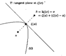
(3) 37. Theorem 3 (A priori estimates for the gradient). Let $\Omega$ \subset \mathbb{R}^{n} be a convex domain. For u_{0} \in W^{1,\infty}( $\Omega$) andfor the transport F underAssumption 1, tet u be a classical solution of (MCF). Then there exists T>0 depending only on n, p, qand \Vert F\Vert_{L_{\mathrm{t} ^{q}L_{x}^{\mathrm{p} ($\Gamma$_{t}) such that. \displaystyle \sup_{0<t<T,x\in\overline{ $\Omega$} \sqrt{1+|du(x,t)|^{2} \leq 2(1+\Vert du_{0}\Vert_{\infty}^{2}) .. (3). With the aid of the Leray‐Schauder fixed point theorem, we can show the time local existence of a classical solution of (MCF). For 0< $\alpha$\leq 1 , define. \displaystyle \Vert F\Vert_{C^{a} ,\mathrm{g}_{( $\Omega$\times \mathrm{R}\times(0,T_{0}) }:=\sup_{( x,z),t ( y,w),s)\in( $\Omega$ \mathrm{x}\mathrm{R})\times(0,T_{0}) \frac{|F(x,zt)-F(y,\mathrm{w},s)|}{x-y|^{ $\alpha$}+|z-w|^{ $\alpha$}+|t-s|^{ $\alpha$/2} . Theorem 4. Let $\Omega$ ditions du_{0} . $\nu$|_{\partial $\Omega$} 0. < $\alpha$. some. \leq 1 .. be a convex domain. Let u_{0} \in W^{1,\infty}( $\Omega$) satisfy compatibility con‐ and let the transport F satisfy \Vert F\Vert_{c^{a},8_{( $\Omega$ \mathrm{x}\mathrm{R}\times(0,T_{0}) } < \infty for some. \subset \mathbb{R}^{n} =. 0. Then, there exists a unique classical solution. u. of (MCF) on. $\Omega$\times \mathbb{R}\times. [0, T) for. 0<T<T_{0}.. In this note, we focus on Theorem 3 since proof of Theorem 4 is more or less standard arguments once we show Theorem 3. Before proving Theorem 3, we discuss Assumption 1 from the point of blowup/scaling arguments. Consider the scale transform for $\lambda$>0. x= $\lambda$ y, u(x, t)= $\lambda$ \mathrm{w}(y, s) , t=$\lambda$^{2}s. Then d_{y}w=(\partial_{y_{1}}w, \ldots, \partial_{y_{n}}w)=du and (MCF) is transformed into. \displaystyle\frac{\partial_{s}\mathrm{w}{\sqrt{1+|d_{y}w|^{2} =\mathrm{d}\mathrm{i}\mathrm{v}_{y}(\frac{d_{y}w{\sqrt{1+|d_{y}w|^{2} \mathrm{I}+$\lambda$F($\lambda$y, $\lambda$w,$\lambda$^{2}s)\cdotn.. To study regularity of du , it is important to investigate the asymptotic behavior of w as $\lambda$\downarrow 0. When. \displaystyle \frac{n}{p}+\frac{2}{q}<1 , then. \Vert $\lambda$ F( $\lambda$ y, $\lambda$ \mathrm{w}, $\lambda$^{2}s)\Vert_{L_{s}^{\mathrm{q} L_{y}^{\mathrm{p} =$\lambda$^{1-\frac{n}{\mathrm{p} \frac{2}{q} \Vert F\Vert_{L_{t}^{q}L_{x}^{p} \rightar ow 0. as. $\lambda$\downarrow 0,. thus the transport is small from the point of blowup/scaling arguments and Assumption 1 is the reasonable condition to obtain the gradient estimates. We remark that Assumption 1 is same assumption to an inhomogeneous term f=f(x, t) to obtain gradient estimates for inhomoge‐ neous heat equations \partial_{t}u-\triangle u=f (see Ladyženskaja‐Solonnikov‐Ural’ceva [9, Theorem 11. 1 in p.211 Figure 2 illustrates the region of (p, q) in Assumption 1. Takasao’s result is almost equivalent to the condition p> n+1 ,. p > n+1. we obtain F\in. and. q. =. \infty. . In fact, for F. L_{(x,z,t)}^{\infty} ( $\Omega$\times \mathbb{R}\times (0, T_{0}). \in L^{\infty}. (0, T_{0} : W_{(x,z)}^{1,p}( $\Omega$\times \mathbb{R}) under. by the Sobolev inequality. On the other. hand, the transport F might not be bounded in time and space variables in our Assumption 1. Therefore, our results can be regarded as some extension of Takasao’s early result even for the interior gradient estimates. 3. Monotonicity of the metric. Our main task is to establish the up‐to‐the‐boundary monotonicity formula of the Huisken type. Let R := \Vert \mathrm{p}\mathrm{n} ncipal curvatưe of \partial $\Omega$\Vert_{L^{\infty}(\partial $\Omega$)}^{-1} . For r < R , define N_{r} := \{x \in $\Omega$ : dist (x, \partial $\Omega$) <r }. Then for x\in\partial $\Omega$ , there uniquely exists $\zeta$(x) \in\partial $\Omega$ such that dist (x, \partial $\Omega$)= |x- $\zeta$(x)| . We define the reflection point of x with respect to \partial $\Omega$ as \tilde{x}=2 $\zeta$(x)-x . Remark that x+\tilde{x}=2 $\zeta$(x) hence $\zeta$(x) is midpoint between x and \tilde{x} ( \mathrm{s}\mathrm{e}\mathrm{e} Figure 3)..

(4) 38. FIGURE 2. Region of (p, q) in Assumption 1. Our assumption is the region of oblique lines and Takasao’s assumption is almost equivalent to the bold line.. -. x). FIGURE 3. The reflection point of x\in $\Omega$\cap N_{r} with respect to \partial $\Omega$ is denoted by. Fix a radially symmetric smooth cut‐off function $\eta$= $\eta$(r)= $\eta$(|(x, z. \tilde{x}.. such that. 0\displaystyle \leq $\eta$\leq 1, \frac{\partial $\eta$}{\partial r}\leq 0, \mathrm{s}\mathrm{p}\mathrm{t} $\eta$\subset B_{R/2}, $\eta$=1\mathrm{o}\mathrm{n}B_{R/4}. For. 0. < t < s <. T_{0} and (x, z) , (y, w). \in. N_{R} \times \mathbb{R} , define the. n. ‐dimensional backward and. reflected backward heat kernels as. $\rho$_{(y,w,s)}(x, z,t):=\displaystyle \frac{1}{(4 $\pi$(s-t) ^{\frac{n}{2} }\exp(-\frac{|x-y|^{2}+|z-w|^{2} {4(s-t)}) \displaystyle \tilde{ $\rho$}_{(y,w,s)}(x, z,t):=$\rho$_{(y,w,s)}(\tilde{x}, z, t)=\frac{\prime 1}{(4 $\pi$(s-t) ^{\frac{n}{2} }\exp(-\frac{|\overline{x}-y|^{2}+|z-w|^{2} {4(s-t)}) ,. \langle4). .. For fixed 0<t<s and (x, z) , (y, w)\in N_{R}\times \mathbb{R} , define a truncated version of $\rho$ and \tilde{$\rho$} as (5). $\rho$_{1}=$\rho$_{1}(x, z,t) := $\eta$(|(x, z)-(y, w)|)$\rho$_{(y,w,s)}(x, z, t) $\rho$_{2}=$\rho$_{2}(x, z,t) := $\eta$(|(\overline{x}, z)-(y, w)|)\tilde{ $\rho$}_{(y,w,s)}(x, z, t). ,. .. To derive Huisken’s monotonicity formula, (6). \displaystyle \frac{(e\cdot D $\rho$)^{2} { $\rho$}+\mathrm{t}\mathrm{r}( I-e\otimes e)D^{2} $\rho$)+\partial_{t} $\rho$=0. is the crucial identity, where. e. \in. \mathbb{R}^{n+1} with. reflected backward heat kernel was obtained.. |e|. =. 1.. In [11], a similar inequality for the.

(5) 39. Lemma 5 ([11. There is a constant C_{2}. \tilde{ $\rho$}=\tilde{ $\rho$}_{(y,w,s)}(x, z, t) (7). >. 0. such that for. e. \in. \mathbb{R}^{n+1} with. |e|. =. 1. and. ,. \displaystyle \frac{(e\cdot D\tilde{ $\rho$})^{2} {\tilde{ $\rho$} +\mathrm{t}\mathrm{r}( I-e\otimes e)D^{2}\tilde{ $\rho$})+\partial_{t}\tilde{ $\rho$}\leq C_{2}(\frac{|\tilde{x}-y|+|z-w|}{s-t}+\frac{(|\tilde{x}-y|+|z-w|)^{3} {(s-t)^{2} )\tilde{ $\rho$}. for 0<t<s and (x, z) , (y, w)\in N_{R/2}\times \mathbb{R}.. We also use the following identity about the second fundamental form of $\Gamma$_{t}. Lemma 6. Let u be a classical solution of (MCF) and let v (8). :=\sqrt{1+|du|^{2}}.. Then. \displaystyle \partial_{t}v-$\Delta$_{$\Gamma$_{\mathrm{t} v- (\frac{du}{v}\cdot dv)\frac{\partial_{t}u}{v}=-|A_{t}|^{2}v-\frac{2|D_{$\Gamma$_{t} v|^{2} {v}+du\cdot d(F\cdot n). ,. where D_{$\Gamma$_{\mathrm{t} , \triangle_{$\Gam a$_{\mathrm{t} , and A_{t} are the surface gradient, the surface Laplacian, and the secondfunda‐ mentalform associated to $\Gamma$_{t} , respectively. Proof of Lemma 6 is given in Takasao [14]. A key identity is. -\displaystyle \triangle_{$\Gamma$_{t} v+|A_{t}|^{2}v+\frac{2|D_{$\Gamma$_{\mathrm{t} v|^{2} {v}-v^{2}(D_{$\Gamma$_{\mathrm{t} h\cdot e_{n+1})=0 given by Ecker‐Huisken [5].. We use the following identities which give a relationship between the normal derivative of. |du|^{2} and the second fundamental form ofthe boundary. It is a simple observation and has been. used in a number of papers (see for [2, 10, 13. Proof of the following Lemma 7 is given in. [11, Lemma 4.2] or Tonegawa [15, Lemma 3.1] for instance. Lemma 7. Let. $\Omega$. be a convex domain and let. u\in C^{2}(\overline{ $\Omega$}) satisfy du\cdot i\prime|_{\partial $\Omega$}=0 . Then. (d|du|^{2}\cdot $\nu$)|_{\partial( $\Omega$ \mathrm{x}\mathrm{N})}\leq 0.. (9). Now we give the boundary monotonicity formula of Huisken type with the transport F.. Proposition 8 (Boundary monotonicity formula). Let u be a classical solution of (MCF) and let v. :=\sqrt{1+|du|^{2}}.. Then for (y, w)\in N_{R/4}\times \mathbb{R} and 0<t<s,. \displaystyle \frac{d}{dt}\int_{$\Gamma$_{t} v($\rho$_{1}+$\rho$_{2})d\mathscr{H}^{n}\leq-\int_{$\Gamma$_{\mathrm{t} ($\rho$_{1}+$\rho$_{2})(|A_{t}|^{2}v+\frac{2|D_{$\Gamma$_{t} v|^{2} {v}-du\cdot d(F\cdot n) (10). +\displaystyle \frac{1}{4}\int_{$\Gamma$_{t} v($\rho$_{1}+$\rho$_{2})(F\cdot n)^{2}d\mathscr{H}^{n} +C_{3}\displaystyle \mathscr{H}^{n}($\Gamma$_{t})+C_{4}(s-t)^{-\frac{3}{4} \int_{$\Gamma$_{\mathrm{t} v($\rho$_{1}+$\rho$_{2})d\mathscr{H}^{n} +C_{5}\displayst le\int_{$\Gam a$_{t}\cap\mathrm{s}\mathrm{p}\mathrm{t}$\rho$_{2}vd\mathscr{H}^{n},. where C3, C_{4}, C_{5}>0 are positive constants depending only on. n. and R.. d\mathscr{H}^{n}.

(6) 40. Proof. For i=1 , 2. (11). \displaystyle\frac{d}{dt}\int_{\mathrm{t} v$\rho$_{i}d\mathscr{H}^{n}=\frac{d}{dt}\int_{$\Omega$}v$\rho$_{i}vdx =\displaystyle \int_{ $\Omega$}\partial_{t}v$\rho$_{i}vdx+\int_{ $\Omega$}v\partial_{x_{n+1} $\rho$_{i}\partial_{t}uvdx +\displaystyle \int_{ $\Omega$}v\partial_{t}$\rho$_{i}vdx+\int_{ $\Omega$}v$\rho$_{i}\partial_{t}vdx =\displaystyle \int_{$\Gamma$_{t} (\partial_{t}v$\rho$_{i}+v\partial_{t}$\rho$_{i}+v\partial_{x_{n+1} $\rho$_{i}\partial_{t}u)d\mathscr{H}^{n}+\int_{ $\Omega$}$\rho$_{i}du\cdot d(\partial_{t}u)dx,. where we denote $\rho$_{i}=$\rho$_{i}(x, u(x, t), t) for simplicity. Using the integration by parts,. \displaystyle \int_{ $\Omega$}$\rho$_{i}du\cdot d(\partial_{t}u)dx=\int_{ $\Omega$}$\rho$_{i}\frac{du}{v}\cdot d(\partial_{t}u)vdx =-\displaystyle \int_{ $\Omega$}dv\cdot\frac{du}{v}$\rho$_{i}\partial_{t}udx-\int_{ $\Omega$}(d$\rho$_{i}+\partial_{x_{n+1} $\rho$_{i}du)\cdot\frac{du}{v}\partial_{t}u. vdx. -\displaystyle\int_{$\Omega$} \rho$_{i}\mathrm{d}\mathrm{i}\mathrm{v}(\frac{du}{v)\partial_{t}u =-\displaystyle \int_{$\Gam a$_{t} (dv\cdot\frac{du}{v})$\rho$_{i}\frac{\partial_{t}u}{v}d\mathscr{H}^{n}-\int_{$\Gam a$_{\mathrm{t} ( d$\rho$_{i}+\partial_{x_{n+1} $\rho$_{i}du)\cdot\frac{du}{v})\partial_{t}ud\mathscr{H}^{n} +\displaystyle\int_{$\Gam a$_{t}$\rho$_{i}h\partial_{t}ud\mathscr{H}^{n}, vdx. where. h=-\displaystyle \mathrm{d}\mathrm{i}\mathrm{v}(\frac{d\mathrm{u} {v}) . Note that. \displaystyle \partial_{x_{n+1} $\rho$_{i}v-\partial_{x_{n+1} $\rho$_{i}\frac{|du|^{2} {v}-d$\rho$_{i}\cdot\frac{du}{v}=\partial_{x_{n+1} $\rho$_{i}\frac{1}{v}-d$\rho$_{l}\cdot\frac{du}{v}=(D$\rho$_{i}\cdot n) where. D=(d, \partial_{x_{n+1}})=(\partial_{x_{1}}, \ldots, \partial_{x_{n+1}}) .. ,. Hence we obtain. \displaystyle\frac{d}{dt}\int_{$\Gam a$_{t} v$\rho$_{i}d\mathscr{H}^{n}=\int_{$\Gam a$_{\mathrm{t} \partial_{t}v$\rho$_{i}d\mathscr{H}^{n}+\int_{$\Gam a$_{t} v\partial_{t}$\rho$_{i}d\mathscr{H}^{n}+\int_{$\Gam a$_{t} v(D$\rho$_{i}\cdotn)\frac{\partial_{t}u {v}d\mathscr{H}^{n} -\displaystyle\int_{$\Gam a$_{\mathrm{t} (dv\cdot\frac{du}{v})$\rho$_{i}\frac{\partial_{t}u {v}d\mathscr{H}^{n}+\int_{$\Gam a$_{t} v$\rho$_{i}h\frac{\partial_{t}u {v}d\mathscr{H}^{n}. Using (MCF), we obtain \partial_{t}u=(-(H\cdot n)+(F\cdot n))v and. (v(D$\rho$_{i}\displaystyle \cdot n)+v$\rho$_{i}(H\cdot n) \frac{\partial_{t}u}{v}. =(v(D$\rho$_{i}\cdot n)+v$\rho$_{i}(H\cdot n))(-(H\cdot n)+F\cdot n). =-v$\rho$_{i}|H-\displaystyle \frac{D^{\perp}$\rho$_{i} {$\rho$_{i} |^{2}+v\frac{|D^{\perp}$\rho$_{i}|^{2} {p_{i} -v(D^{\perp}$\rho$_{i}\cdot H) +v$\rho$_{i} ( \displaystyle \frac{D^{\perp}$\rho$_{i} {$\rho$_{i} -H) . n)(F\cdot n) \displaystyle \leq v\frac{|D^{\perp}$\rho$_{i}|^{2} {$\rho$_{i} -v(D^{\perp}$\rho$_{i}\cdot H)+\frac{1}{4}vp_{i}(F\cdot n)^{2},.

(7) 41. where. D^{\perp}$\rho$_{i}=(D$\rho$_{i}\cdot n)n .. Therefore,. \displaystyle\frac{d}{dt}\int_{$\Gam a$_{t} v$\rho$_{i}d\mathscr{H}^{n}\leq\int_{\mathrm{t} \partial_{t}v$\rho$_{i}d\mathscr{H}^{n}-\int_{$\Gam a$_{t} (dv\cdot\frac{du}{v})$\rho$_{i}\frac{\partial_{t}u {v}d\mathscr{H}^{n} +\displaystyle \int_{$\Gam a$_{t} v(\partial_{t}$\rho$_{i}+\frac{|D^{\perp}$\rho$_{l}|^{2} {$\rho$_{i} -(D^{\perp}$\rho$_{i}\cdot H) d\mathscr{H}^{n} +\displaystyle \frac{1}{4}\int_{$\Gam a$_{t} v$\rho$_{i}(F\cdot n)^{2}d\mathscr{H}^{n}. According to the divergence theorem on $\Gam a$_{\mathrm{t} ,. -\displaystyle\int_{$\Gam a$_{t} v(D^{\perp}$\rho$_{i}\cdotH)d\mathscr{H}^{n}=\int_{$\Gam a$_{\mathrm{t} \mathrm{d}\mathrm{i}\mathrm{v}_{$\Gam a$_{\mathrm{t} (vD$\rho$_{i})d\mathscr{H}^{n}-\int_{\partial$\Gam a$_{t} v(D$\rho$_{i}\cdot$\nu$)d\mathscr{H}^{n-1} =\displaystyle \int_{$\Gamma$_{t} D_{$\Gamma$_{t} v\cdot D$\rho$_{i}d\mathscr{H}^{n}+\int_{t}v\mathrm{t}\mathrm{r}( I-n\otimes n)D^{2}$\rho$_{i})d\mathscr{H}^{n} -\displaystyle\int_{\partial$\Gam a$_{\mathrm{t} v(D$\rho$_{i}\cdotv)d\mathscr{H}^{n-1} =-\displaystyle\int_{$\Gam a$_{t} $\rho$_{i}\triangle_{$\Gam a$_{t} vd\mathscr{H}^{n}+\int_{$\Gam a$_{\mathrm{t} v\mathrm{t}\mathrm{r}( I-n\otimesn)D^{2}$\rho$_{i})d\mathscr{H}^{n} +\displaystyle\int_{\partial$\Gam a$_{t} ($\rho$_{i}(D_{$\Gam a$_{\mathrm{t} v\cdot\mathrm{v})-v(D$\rho$_{i}\cdot$\nu$) d\mathscr{H}^{n-1} ( $\nu$, 0) , \mathrm{d}\mathrm{i}\mathrm{v}_{$\Gam a$_{t} is the surface divergence, \triangle_{$\Gamma$_{t} is the surface Laplacian, and D_{$\Gamma$_{t} (I-\mathrm{v}\otimes \mathrm{v})D is the surface gradient associated to $\Gamma$_{t} . Remarking that. where. \mathrm{v}. =. =. D_{$\Gamma$_{t} v=(dv, 0)+\displaystyle \frac{(du,dv)}{\sqrt{1+|du|^{2} n, we obtain D_{$\Gamma$_{t} v\cdot $\nu$. =. dv\cdot \mathrm{v}. from the Neumann boundary condition. Using (6) and (7), we. obtain. (12). \displaystyle \frac{|D^{\perp}$\rho$_{1}|^{2} {$\rho$_{1} +\mathrm{t}\mathrm{r}( I-n\otimes n)D^{2}$\rho$_{1})+\partial_{t}p_{1} \leq C_{6}. and. (13). \displaystyle\frac{|D^{\perp}$\rho$_{2}|^{2} {$\rho$_{2} +\mathrm{t}\mathrm{r}( I-n\otimesn)D^{2}$\rho$_{2})+\partial_{t}$\rho$_{2} \displaystyle \leq C_{7}(\frac{|\tilde{x}-y|+|z-w|}{s-t}+\frac{(|\tilde{x}-y|+|z-w|)^{3} {(s-t)^{2} )$\rho$_{2}+C_{8}. for some constants C_{6} , C7, C_{8}>0 depending only on n and R. To compute the integrations of (13), we decompose the integrations as. \displaystyle \int_{$\Gamma$_{t} v\frac{|\tilde{x}-y|+z-w|}{s-t}$\rho$_{2}d\mathscr{H}^{n}\leq\int_{$\Gamma$_{\mathrm{t} \cap\{|\overline{x}-y|+z-w|\leq(s-t)^{1}\} \mathrm{z}v\frac{|\tilde{x}-y|+z-w|}{s-t}$\rho$_{2}d\mathscr{H}^{n} +\displaystyle \int_{1}$\Gamma$_{t}\cap\{|\overline{x}-y|+|z-w|\geq(s-t)\mathrm{z}\}v\frac{|\tilde{x}-y|+|z-w|}{s-t}$\rho$_{2}d\mathscr{H}^{n} =:I_{1}+I_{2},.

(8) 42. and. \displaystyle \int_{$\Gam a$_{t} v\frac{(|\tilde{x}-y|+z-\mathrm{w}|)^{3} {(s-t)^{2} $\rho$_{2}d\mathscr{H}^{n}\leq\int_{$\Gam a$_{\mathrm{t} \cap\{|\overline{x}-y|+z-w|\leq(s-t)} v\displaystyle \frac{(|\tilde{x}-y|+z-\mathrm{w}|)^{3} {(s-t)^{2} $\rho$_{2}d\mathscr{H}^{n} +\displaystyle \int_{ $\iota$\cap\{|\overline{x}-y|+|z-w|\geq(s-t)\} \# v\frac{(|\tilde{x}-y|+|z-w|)^{3} {(s-t)^{2} $\rho$_{2}d\mathscr{H}^{n} fi. =:I_{3}+I_{4}.. I_{1} and I3 are estimated as. I_{1}\displaystyle\leq(s-t)^{-\frac{3}{4} \int_{$\Gam a$_{\mathrm{t} v$\rho$_{2}d\mathscr{H}^{n}, I_{3}\displaystyle \leq(s-t)^{-\frac{3}{4} \int_{$\Gamma$_{t} v$\rho$_{2}d\mathscr{H}^{n}.. (14). I_{2} and I_{4} are estimated as. I_{2}\displaystyle \leq\frac{4 $\pi$}{(4 $\pi$(s-t) ^{1+\frac{n}{2} e^{-\frac{1}{4\sqrt{}s-t} \int_{$\Gam a$_{\mathrm{t} \cap \mathrm{s}\mathrm{p}\mathrm{t}$\rho$_{2} v(|\tilde{x}-y|+z-w|)d\mathscr{H}^{n} \displaystyle \leq C_{9}\int_{$\Gam a$_{\mathrm{t} \cap \mathrm{s}\mathrm{p}\mathrm{t}$\rho$_{2} v(|\tilde{x}-y|+z-w|)d\mathscr{H}^{n}, I_{4}\displaystyle\leq\frac{(4$\pi$)^{2} {(4$\pi$(s-t) ^{2+\frac{n}{2} e^{-\frac{1}{4\sqrt{s-\mathrm{t} }\int_{$\Gam a$_{t}\cap\mathrm{s}\mathrm{p}\mathrm{t}$\rho$_{2} v(|\tilde{x}-y|+z-w|)^{3}d\mathscr{H}^{n} \displaystyle\leqC_{9}\int_{$\Gam a$_{\mathrm{t} \cap\mathrm{s}\mathrm{p}\mathrm{t}$\rho$_{2} v(|\tilde{x}-y|+z-w|)^{3}d\mathscr{H}^{n}. (15). for some constant C_{9}>0 depending only on n . Using (14), (15), |\tilde{x}-y|+|z-w| \leq R when (x, z)\in spt $\rho$_{2} , and D($\rho$_{1}+$\rho$_{2})\cdot \mathrm{v}|_{\partial $\Omega$}\equiv 0 , we obtain. \displaystyle\frac{d}{dt}\int_{$\Gam a$_{\mathrm{t} v($\rho$_{1}+$\rho$_{2})d\mathscr{H}^{n}\leq\int_{$\Gam a$_{t} ($\rho$_{1}+$\rho$_{2})(\partial_{t}v-\triangle_{$\Gam a$_{\mathrm{t} v-(dv\cdot\frac{du}{v})\frac{\partial_{t}u {v}). d\mathscr{H}^{n}. +\displaystyle \frac{1}{4}\int_{$\Gamma$_{t} ($\rho$_{1}+$\rho$_{2})v(F\cdot n)^{2}d\mathscr{H}^{n} +(C_{6}+C_{8})\displaystyle \mathscr{H}^{n}($\Gamma$_{t})+2(s-t)^{-\frac{3}{4} \int_{$\Gamma$_{\el } v$\rho$_{2}d\mathscr{H}^{n} +2C_{10}\displaystyle\int_{$\Gam a$_{t}\cap\mathrm{s}\mathrm{p}\mathrm{t}$\rho$_{2} vd\mathscr{H}^{n}+\int_{\partial$\Gam a$_{t} ($\rho$_{1}+\cdot$\rho$_{2})(D_{$\Gam a$_{t} v\cdot\mathrm{v})d\mathscr{H}^{n-1}. where C_{10}=C_{9}(R+R^{3}) . Using (8) and (9), we obtain (10) with C_{5}=2C_{10}.. 4. Gradient estimates. We deduce the integral estimates for the transport terms.. c_{3}=c_{6}+c_{8}, C_{4}=2 ,. and \square.

(9) 43. Lemma 9. Let v. F. \in\ovalbox{\t \smal REJECT} {}_{x}L_{t}^{q}($\Gamma$_{t}) with. 1-\displaystyle \frac{n}{p}-\frac{2}{q}. >. 0,. u. be a classical solution of (MCF), and. :=\sqrt{1+|du|^{2}}. Then there is a constant C_{11}>0 depending only on. n, p, q. , and T_{0} such that. \displaystyle \int_{0}^{s}dt\int_{$\Gamma$_{t} ($\rho$_{1}+$\rho$_{2})du\cdot d(F\cdot n)d\mathscr{H}^{n}+\frac{1}{4}\int_{0}^{s}dt\int_{$\Gamma$_{\mathrm{t} v(p_{1}+$\rho$_{2})(F\cdot n)^{2}d\mathscr{H}^{n} \displaystyle \leq\frac{1}{2}\int_{0}^{s}dt\int_{$\Gam a$_{t} ($\rho$_{1}+$\rho$_{2})|A_{t}|^{2}vd\mathscr{H}^{n}+\int_{0}^{s}dt\int_{$\Gam a$_{t} ($\rho$_{1}+$\rho$_{2})\frac{|D_{$\Gam a$_{t} v|^{2} {v}d\mathscr{H}^{n}. (16). +C_{11}\Vert v\Vert_{\infty}^{3}(1+\Vert F\Vert_{L_{x}^{\mathrm{p} L_{\mathrm{t} ^{q}($\Gamma$_{t})})^{2}. for 0<s<T_{0}.. Proof. We focus on the integral estimates of ($\rho$_{1}+$\rho$_{2})du\cdot d(F\cdot n) . For simplicity, set \overline{ $\rho$}:= $\rho$_{1}+$\rho$_{2} . Then. Here. \displaystyle \int_{$\Gamma$_{t} \overline{ $\rho$}(du\cdot d(F\cdot n) d\mathscr{H}^{n}=\int_{ $\Omega$}\overline{p}(du\cdot d(F\cdot n) vdx =-\displaystyle \int_{ $\Omega$}(\overline{ $\rho$}\triangle uv+(du\cdot d\overline{ $\rho$})v+\overline{ $\rho$}(du\cdot dv) (F\cdot n)dx =-\displaystyle \int_{$\Gamma$_{t} (\overline{ $\rho$}\triangle u+(du\cdot d\overline{ $\rho$})+\overline{ $\rho$}(\frac{du}{v}\cdot dv) (F\cdot n)d\mathscr{H}^{n}.. h=-\displaystyle \mathrm{d}\mathrm{i}\mathrm{v}(\frac{du}{v}) =-\frac{1}{v}\triangle u+\frac{1}{v^{2} (du\cdot dv). hence,. ;. \displaystyle\int_{$\Gam a$_{\mathrm{t} \overline{$\rho$}du\cdotd(F\cdotn)d\mathscr{H}^{n}=\int_{\mathrm{t} \dot{\overline{$\rho$} vh(F\cdotn)d\mathscr{H}^{n} -2\displaystyle \int_{$\Gam a$_{t} \overline{ $\rho$}(\frac{du}{v}\cdot dv)(F\cdot n)d\mathscr{H}^{n} -\displaystyle \int_{$\Gamma$_{t} (du\cdot d(\overline{ $\rho$}(x, u, t) (F\cdot n)d\mathscr{H}^{n} =:I_{1}+I_{2}+I_{3}.. We focus on an integral estimate of I3. Because. |du\cdot d(\overline{ $\rho$}(x,u, t =|du\cdot d\overline{ $\rho$}+|du|^{2}\overline{ $\rho$}_{x_{n+1}}|\leq v^{2}|D\overline{ $\rho$}|, we obtain. |I_{3}| \displaystyle \leq\int_{$\Gam a$_{t} v^{2}|D\overline{ $\rho$}|F\cdot n|d\mathscr{H}^{n}.. Then using the Hölder inequality, (17). where. \displaystle\int_{0}^s|I_{3}|dt\leq\Vertv\Vert_{\infty}^{2 (\int_{0}^sdt(\int_{$\Gam a$_{\mathrm{t} |D\overline{$\rho$}|^{p\ rime}d\mathscr{H}^{n)^{p}\mathrm{g}_7')^{\neg}q1\VertF\Vert_{L x}^{\mathrm{p}L_{t}^\mathrm{q}($\Gam a$_{\mathrm{t}),. \displaystyle \frac{1}{p}+\frac{1}{p}=1 and \displaystyle \frac{1}{q}+\frac{1}{q}=1 . Using the convexity of $\Omega$,. |\tilde{x}-y| \geq|x-y| ; hence,. |D\displaystyle \overline{ $\rho$}|\leq C_{12}\frac{1}{(s-t)^{\frac{1}{2}+\frac{n}{2} \exp(-\frac{|x-y|^{2}+|z-w|^{2} {8(s-t)}. ,.

(10) 44. where C_{12}>0 is some constant depending only on n . Thus we have. \displaystyle\int_{$\Gam a$_{t} |D\overline{$\rho$}|^{p\prime}d\mathscr{H}^{n}\leqC_{12}^{p'}(s-t)^{-\acute{\mathrm{L} -\frac{np'}{2}+\frac{n}{2} 2. ;. or. (\displayst le\int_{0}^{sdt(\int_{$\Gam a$_{\mathrm{t} |D\overline{$\rho$}|^{p\ rime}d\mathscr{H}^{n})^{+_p}')^{$\Gam a$^{1} \leqC_{1} _{2}T_{0}^{\frac{1}2(1-\frac{n}p-\frac{2}\mathrm{q})<\infty.. Therefore, using (17) we obtain. \displaystyle\int_{0}^{s}|I_{3}|dt\leqC_{1}{_2}T_{0}^{\frac{1}{2}-\frac{n}{2\mathrm{p}-\frac{1}{\mathrm{q} \Vertv\Vert_{\infty}^{2}\VertF\Vert_{L_{x}^{\mathrm{p}L_{\mathrm{t}^{q}($\Gam a$_{t}).. (18). As the similar argument as above, we also obtain. \displaystyle \int_{0}^{s}(|I_{1}|+|I_{2}|)dt+\int_{0}^{s}dt\int_{$\Gamma$_{t} v($\rho$_{1}+$\rho$_{2})(F\cdot n)^{2}d\mathscr{H}^{n}. \displaystyle\leq\frac{1}{2}\int_{0}^{s}dt\int_{$\Gam a$_{t}\overline{$\rho$}|A_{t}|^{2}vd\mathscr{H}^{n}+\int_{0}^{s}dt\int_{$\Gam a$_{t}\overline{$\rho$}\frac{|D_{$\Gam a$_{\mathrm{t} v|^{2}{v}d\mathscr{H}^{n}. (19). +C_{13}T_{0}^{1-\frac{n}{\mathrm{p} -\frac{2}{\mathrm{q} \Vertv\Vert_{\infty}^{3}\VertF\Vert_{L_{x}^{p}L_{t}^{\mathrm{q} ($\Gam a$_{\mathrm{t} ) ^{2}. for a positive constant Cl3. >0. depending only on n, p, q . Combining (18) and (19), we obtain \square. (16).. Proof of Theorem 3. We only focus on the gradient estimates near the boundary \partial $\Omega$ . Fix (y, w) \in N_{R/4} \times \mathbb{R} and 0 < T < T_{0} . For 0 < t < s < T , using (10) and (16) and \mathscr{H}^{n}($\Gamma$_{t})\leq\Vert v\Vert_{\infty}| $\Omega$|,. \displaystyle\frac{d}{dt}\int_{$\Gam a$_{\el} v($\rho$_{1}+$\rho$_{2})d\mathscr{H}^{n}. \displaystyle\leqC_{4}(s-t)^{-\frac{3}{4} \int_{$\Gam a$_{t} v($\rho$_{1}+$\rho$_{2})d\mathscr{H}^{n}+C_{14}(1+\VertF\Vert_{L_{x}^{\mathrm{p} L_{\mathrm{t} ^{\mathrm{q} ($\Gam a$_{\mathrm{t} )} ^{2}\int_{0}^{t'}\Vertv(\cdot, )\Vert_{\infty}^{3}dt, where C_{14} > 0 is a positive constant depending only on inequality for 0<t<s,. n, p, q. and | $\Omega$| . By the Gronwall. \displaystyle \exp(-C_{4}\int_{0}^{t}(s- $\tau$)^{-\frac{3}{4} d $\tau$)\int_{$\Gamma$_{t} v($\rho$_{1}( x, z), t)+p_{2}( x, z), t) d\mathscr{H}^{n} \displaystyle \leq\int_{$\Gamma$_{0} v(x, 0)($\rho$_{1}( x, z), 0)+$\rho$_{2}( x, z), 0) d\mathscr{H}^{n} +C_{14}(1+\displaystyle \Vert F\Vert_{L_{x}^{\mathrm{p} L_{\mathrm{t} ^{\mathrm{q} ($\Gam a$_{t}) ^{2}\int_{0}^{t}\exp(4C_{4}( \mathcal{S}- $\tau$)^{\frac{1}{4} -s^{\frac{1}{4} ) \Vert v(\cdot, $\tau$)\Vert_{\infty}^{3}d $\tau$. \displaystyle \leq 2\Vert v(\cdot, 0)\Vert_{\infty}^{2}+C_{1}{ _{4}T(1+\Vert F\Vert_{L_{x}^{\mathrm{p} L_{t}^{\mathrm{q} ($\Gamma$_{\mathrm{t} )} ^{2}\sup_{0<t<T}\Vert v(\cdot, )\Vert_{\infty}^{3}. As. t\rightarrow s ,. we obtain. v(y, s)\displaystyle \leq 2\Vert v(\cdot, 0)\Vert_{\infty}^{2}+C_{14}T(1+\Vert F\Vert_{L_{x}^{p}L^{\mathrm{q} ($\Gamma$_{t})})^{2}\sup_{ }^{t}0<t<T}\Vert v(\cdot, t)\Vert_{\infty}^{3}..

(11) 45. Now, select (y, s) such that v(y, s)=\displaystyle \sup_{0<\mathrm{t}<T}\Vert v(\cdot, t)\Vert_{\infty} . Then,. \displaystyle \sup_{0<t<T}\Vert v(\cdot, t)\Vert_{\infty}\leq 2\Vert v(\cdot, 0)\Vert_{\infty}^{2}+C_{14}T(1+\Vert F\Vert_{L_{x}^{p}L_{\mathrm{t} ^{\mathrm{q} ($\Gamma$_{t})})^{2}\sup_{0<t<T}\Vert v(\cdot, t)\Vert_{\infty}^{3}.. (20). Suppose for a contradiction that there exists. C>2. such that. \displaystyle \sup_{0<t<T}\Vert v(\cdot, t)\Vert_{\infty}>C\Vert v(\cdot, 0)\Vert_{\infty}^{2} for all 0<T<T_{0} . Then (20) implies that. C_{14}\displaystyle \frac{T}{\Vert v(\cdot,0)\Vert_{\infty}^{2} (1+\Vert F\Vert_{L_{x}^{\mathrm{p} L_{\el }^{\mathrm{q} ($\Gamma$_{t}) ^{2}\sup_{0<t<T}\Vert v(\cdot, )\Vert_{\infty}^{3}\geq\frac{\sup_{0<t<T}|v(\cdot, )\Vert_{\infty} {\Vert v(\cdot,0)|_{\infty}^{2} -2>C-2>0,. \square. which is contradiction as taking T\downarrow 0.. References. [1] J. A. Buckland, Mean curvature flow with free boundary on smooth hypersurfaces, J. Reine Angew. Math. 586 (2005), 71−90.. [2] R. G. Casten and C. J. Holland, Instability results for reaction diffusion equations with Neumann boundary conditions, J. Differential Equations 27 (1978), 266‐273. [3] T. H. Colding and W. P. Minicozzi, II, Sharp estimates for mean curvature flow of graphs, J. Reine Angew. Math. 574 (2004), 187‐195.. [4] K. Ecker, Regularity theory for mean curvature flow, Birkhäuser, 2004. [5] K. Ecker and G. Huisken, Interior curvature estimatesfor hypersurfaces ofprescnbed mean curvature, Ann. Inst. H. Poincaré Anal. Non Linéaire 6 (1989), 251−260.. [6] K. Ecker and G. Huisken, Interior estimates for hypersuifaces moving by mean curvature, Invent. Math. 105 (1991), 547‐569.. [7] G. Huisken, Nonparametric mean curvature evolution with boundary conditions, J. Differential Equations 77 (1989), 369‐378.. [8] G. Huisken, Asymptotic behavior for singularities of the mean curvature flow, J. Differential Geom. 31 (1990), 285‐299.. [9] O. A. Ladyženskaja, V. A. Solonnikov, and N. N. Ural’ceva, Linear and quasilinear equations ofparabolic type, American Mathematical Society, 1967. [10] H. Matano, Asymptotic behavior and stability of solutions of semilinear diffusion equations, Publ. Res. Inst. Math. Sci. 15, (1979), 401‐454.. [11] M. Mizuno and Y. Tonegawa, Convergence of the Allen‐Cahn equation with Neumann boundary conditions, SIAM J. Math. Anal. 47 (2015), 1906‐1932.. [12] A. Stahl, Regularity estimates for solutions to the mean curvatureflow with a Neumann boundary condition, Calc. Var. Partial Differential Equations 4 (1996), 385‐407.. [13] P. Stemberg, and K. Zumbrun, Connectivity ofphase boundaries in strictly convex domains, Arch. Rational Mech. Anal. 141 (1998), 375‐400.. [14] K. Takasao, Gradient esĩimates and existence ofmean curvatureflow with transport term, Differential Integral Equations 26 (2013), 141‐154.. [15] Y. Tonegawa, Domain dependent monotonicity formula for a singular perturbation problem, Indiana Univ. Math. J. 52 (2003), 69‐83.. [16] W. P. Ziemer, Weakly differentiable functions, Graduate Texts in Mathematics, vol. 120, Springer‐Verlag, New York, 1989.. (M. Mizuno) DEPARTMENT OF MATHEMATICS, COLLEGE OF SCIENCE AND TECHNOLOGY, NIHON UNI‐ VERSITY. (K. Takasao) GRADUATE SCHOOL OF MATHEMATICAL SCIENCE, THE UNIVERSITY OF TOKYO E‐mail E‐mail. address, M. Mizuno: mizuno@math. cst. nihon -\mathrm{u} . ac. jp address, K. Takasao: takasaoems. \mathrm{u} ‐tokyo. ac. jp.

(12)