Self-sustained flow-oscillations in hole-tone problem (Mathematical Physics and Applications of Nonlinear Wave Phenomena)

Self-sustained flow-oscillations

in

hole-tone

problem

Mikael A.

Langthjem\dagger ,

Masami

Nakano\ddagger

\dagger Faculty

_of

Engineering, Yamagata University,

Jonan

4-chome, Yonezawa-shi,

992-8510

Japan

\ddagger Institute

_of

Fluid Science, Tohoku University,

2-1-1

Katahira, Aoba-ku, Sendai-shi,

980-8577

Japan

Abstract

A method for simulating the hole-tone feedback cycle (Rayleigh’s bird-call), based on a

three-dimensional discrete vortex method, is described in detail. Evaluation ofthe sound

generatedbytheself-sustained flow oscillations is basedonthePoweh-Howetheoryof vortex

sound andthe boundary element method. Emphasisis placedonthedevelopmentofamodel

for the coupling between thevortex-dominated main flow and the acousticfield. Thefinal

part ofthe paper considers, briefly, an analysis based on the method of proper orthogonal decomposition.

Keywords: aeroacoustics; self-sustained flowoscihations; three-dimensionalvortex method;

vortexsound; boundary element method; proper orthogonal decomposition

1

Introduction

Self-sustained

fluid oscihations

can occur

in

a

varietyofpractical applicationswhere

a

shear layer

impinges upon

a

solid structure $[16, 17]$

.

The praeent paper is concerned with such oscillations

in the hole-toneproblem $[15, 2]$, where

a

fluid jet issuingfrom

a

circular holein

a

plate(or kom

a

nozzle) impinges upon

a

(second) plate with

a

similar hole, located alittle downstream from

the nozzle. Self-sustained oscihations of the jet

are

generated, accompanied by sound with

a

definite tone. The

common

teakettle whistle and the

bird-call1

is an example ofutilization of

thephenomenon.

In his $Theo\eta$

of

Sound [15] Rayleigh explained the basic mechanism

as

follows: “When

a

symmetrical

excrescence

reachesthe second plate, it is

unable

to

paes

the

hole

with freedom,and

thedisturbance is thrown back, probably withthe velocityofsound, to the firstplate, where it

gives rise to

a

further disturbance, to grow in its turn duringthe progress of thejet.”

The system isthus

one

wherethesoundgenerationiscaused by synchronization [14] between

the sound-generating flow and the acousticfield.

The dominating frequency $f_{0}$ satisfiesthe criterion

$\ell/u_{c}+l/q=n/f_{0}$

,

(1)

where $\ell$ is the length of the gap between the nozzle exit and the end plate,

$u_{c}$ is the vortex

convection velocity ($u_{c}\approx 0.6u_{0}$, where $u_{0}$ is the

mean

flow velocity), $c_{0}$ is the speed ofsound,

and $n$ is

a

mode number which may take the values

2’ $Z$

1 _1,$\theta\ldots$

.

A change in the value of

$n$

implies

a

corresponding ‘jump’ in thefrequency $f_{0}$

.

A number ofexperimentalstudiesonthe hole toneproblem have been published; particularly noteworthy is the comprehensive work of Chanaud

&Powell

[2]. Theoretical and numerical

studies

are

however few, _{A large body of work has been done on the related,} $tw\sim dimeoional$

edge-tone problem;

some

parallels between the two problems

are

drawn inRef. [2].

As explained in

an

earlier paper [8],

one

of the main purposes of thiswork is to investigate

the effects of non-axisymmetric flow disturbances, imposed ‘mechanically’, in the experiments

via piezoelectric actuatorsplaced around the circumference inside the nozzle. In the numerical

computatioms, this is simulated via

a

deformable nozzle. A threedimensional formulation is

thus necessary. The forcing (control) problem will be considered in

a

future paper. In this

paper the numerical method will be described in detail in

Sections 2-3.

A numerical example

will be presented in Section 4. Finally,

an

analysis based

on

the method of proper orthogonal

decomposition will be described briefly in Section 5.

2

The

discrete

vortex

flow

model

2.1

Vortex

fllament

model

of the jet flow

The shear layer

of

the jet issuing from the nozzleis represented bydiscrete vortex rings. These

rings will be disturbed mechanically at the nozzle exit such that they loose their natural

ax-isymmetricform, and

are

thus represented bythree-dimensional vortex filaments. The induced

velocity $u_{fv}=(u_{1},u_{2}, u_{3})_{fv}$, at position $x=(x_{1}, x_{2}, x_{3})_{i}$ and time $t,$ $homN_{fv}$ vortex rings

represented bythe space

curves

$r_{j}(\xi,t)$, is obtained

&om

the generalized Biot-Savart law [9]

$u_{fv}(x,t)=-\sum_{j=1}^{N_{f\nu}}\frac{\Gamma_{j}}{4\pi}\oint_{C_{j}(}\frac{\{x-r_{j}(\xi,t)\}x\partial r_{j}/\partial\xi q(|x-r_{j}(\xi,t)|/\sigma_{j})}{\epsilon)|x-r_{j}(\xi,t)|^{3}}d\xi$

.

(2)

Here $\Gamma_{j}$ is the strength (circulation) ofthe$j’ th$ vortex ringand $C_{j}(\xi)$ itscontour, described by

the parameter$\xi$

.

The ‘smoothing function’$q(y)$ representsthestructureofthe vortex core, with

$\sigma_{j}(\xi,t)$ being the

core

radius. Iteliminates the logarithmic singularity at$x=r_{j}$

,

and smoothes

out the vorticitydistribution. In the present work the Rosenhead-Moore function

$\dot{q}(\kappa)=\frac{\kappa^{3}}{(\kappa^{2}+\alpha)^{3}z}$ (3)

ischosen [9]. If(2)and(3)

are

to give the

same

single-ring speed

as

theGaussian

core

distribution

$\varpi(\rho)=\pi^{-g}2\exp(-\rho^{2})$, (4)

with the corresponding smoothingfunction

$q(n)=4 \pi\int_{0}^{\kappa}\varpi(\rho)\rho^{2}d\rho$, (5)

then the parameter $\alpha$ should have the value

0.413

[1]. This value is accordingly used in the

numerical simulations.

2.2

Representation

of

solid surfaces

The solidsurfaces

are

represented byrectilinear vortexring ‘panels’, made up of fourstraight

vortex filaments,

as

indicated inFig. 1. The velocity induced from such

a

vortex panel

can

be

$y_{j+1},$ $j=1,$$\ldots,$$4$, where $y_{5}$ $:=y_{1}$

.

Following the approach of

Katz&Plotkin

[6], the velocity

induced from $N_{bv}$ panels is

$u_{bv}(x)=\sum_{j=1}^{N_{bv}}\sum_{i=1}^{4}\frac{\Gamma_{j}}{4\pi}[\frac{r_{i}\cross r_{|+1}}{|r_{i}xr_{i+1}|^{2}}r_{0}\cdot(\frac{r_{i}}{r_{i}}-\frac{r_{i+1}}{r_{i+1}})]_{j}$ , (6)

where $r_{i}=y_{i}-x$ and $r_{0}=r_{i}-r_{i+1}$ (and r5 $:=r_{1}$). The

mean

jet flow is also provided by

a number of such vortexpanels, placed

on

the ‘back’ ofthe nozzle tube, and by

a

single point

source, which providesthe induced velocity

$u_{\mu}(x)=\frac{\sigma}{4\pi}\frac{r}{r^{8}}$

.

(7)

Here $\sigma$ is the

source

strength,

$r=x-y$

and $r=|r|$

.

The velocity at

an

arbitrary point _$x$ is thus given by

$u(x)=u_{fv}+u_{bv}+u_{ps}$

.

(8)

The strengths ofthe bound vortex panels, and the single point source,

are

dictated bythe

boundaryconditions and the

mean

jet velocity.

Figure 1: Solid surfaces represented by vortex panels. The

mean

flow-generating pane18

are

placed at $z=0.O$, the nozzle exit at $z=2.5$

,

and the endplate at $z=3.5$

.

First, it isrequired that the inviscid boundarycondition of

zero

normal velocity issatisfied

on

the exit pipe (surfaoe 2’) and the end plate (’surface3’), i.e.

$u_{n}(x_{1\dot{0}}^{cpk})=0$

,

$i=1,$ $\ldots,$

$N_{\theta k}$, $j=1,$

$\ldots,$$N_{rk}$, $k=2,3$, (9)

where$x_{i_{\dot{O}}}^{cpk}$

are

control points located in the center of the vortex panels, $N_{\theta k}$ is the number of

panels incircumferential direction, and $N_{rk}$ the number ofpanels in radial direction.

Second, the velocitydistribution

on

the

mean

flow-providingupstream end ofthe exit pipe (’surface 1’) is required to beuniform. This is obtained bythe following two conditions:

$u_{n}(x_{i_{\dot{\theta}}}^{cp1})-u_{n}(x_{1+1,j}^{cp1})=0$, $i=1,$

$\ldots,$$N_{\theta 1}-1$, $j=1,$$\ldots,$$N_{r1}$, (10)

$u_{n}(x_{1\dot{\theta}}^{cp1})-u_{\mathfrak{n}}(x_{i_{\dot{\theta}}+1}^{cp1})=0$

,

_{$i=N_{\theta 1}-1$}

,

$j=1,$

$\ldots,$$N_{r1}$

.

(11)

Equation (10) expresses

a zero

velocityjump

across

anytwo adjacent pane18 inradialdirection,

at any circumferential station. Equation (11) expresses

a zero

velocityjump

across

any two

adjacent panels in circumferentialdirection, for

one

particular radius.

The third and final condition is the specification of the

mean

velocity at

a

specified point

$x_{*}$;

The conditions (9)$-(12)$ constitute $\sum_{k}(N_{\theta k}\cross N_{rk})+1$ equations with the

same

number of

unknowns. The matrix equation system corresponding to these equations takes the form

Ar$=b$

.

₍₁₃₎

Here the matrixAcontains theinfluence coefficients and$\Gamma$the unknown$vortex/source$strengths.

The vector $b$contains the inducedvelocities from the freevortices; the elements

are

given by

$b_{j}=- \sum_{i=1}^{N_{fv}}$害

{ufv}

, (14)

where $S\{\}$repraeents the ‘operations’ defined by (9)$-(12)$

.

2.3

Vortex shedding

mechanism

The rate of continuous sheddingof circulation $\gamma$ from the nozzle is given by

$\frac{d\gamma}{dt}=_{R}^{1}(u_{t-}^{2}-u_{t+}^{2})$, (15)

where $u_{t-}$ isthe (tangential) velocity at thepipe exit, $z_{exit}$ say,

on

the inner surface, and $u_{t+}$ is

the corresponding velocity

on

theouter surface. This equation

can

be obtain\’e by integrating

the tangential component of the Euler equations

over

the tube surface, and using the Kutta

condition, which demands that thepressure alittle abovethe nozzle edge equalsthe pressure

a

little below.

In thesimulation

a

vortex ringisreleased at everytimestep, at the position

$z_{z^{1}e1}=z_{exit}+ \frac{1}{2}\Delta t(u_{t-}+u_{t+})$

.

(16)

Itsstrength is obtained from (15)

as

$\Gamma=arrow 1\Delta t2(u_{t-}^{2}-u_{t+}^{2})$

.

(17)

The vortexrings, described by the space

curves

$r_{j}(\xi, t)$,

are

discretized by employing $N_{mp}$

marker points

on

each curve, connected via cubic splines. The positions of the marker points

onthe shed vortex rings,describedbythevectors$r_{m}(\zeta_{n}, t)$

, are

updated by solving numerically

the systemofordinarydifferential equations

$\frac{dr_{m}(\zeta_{n},t)}{dt}$ _$=$

$- \sum_{j=1}^{N_{fv}}\frac{\Gamma_{j}}{4\pi}\oint_{C_{j}(\xi)}\frac{\{r_{m}(\zeta_{n},t)-r_{j}(\xi,t)\}x\partial r_{j}/\partial\xi}{\{|r_{m}(\zeta_{n},t)-r_{j}(\xi,t)|^{2}+\alpha\sigma_{j}^{2}(\xi,t)\}^{\frac{3}{2}}}d\xi$ (18)

$+$ $u_{bv}(\zeta_{n},t)+u_{p\epsilon}(\zeta_{\mathfrak{n}},t)$, $m=1,$

$\ldots,$$N_{fv}$

,

$n=1,$$\ldots,$$N_{cp}$

.

To this end the fourth-order Runge-Kutta method is applied. The integrations

over

$C_{j}(\zeta)$ in

(18)

are

carriedout using

Gaussian

quadrature [7].

Exceptfor the viscous effect simulatedbythe Kuttacondition,thecomputations

are

basically

inviscid. This

means

that the vortex rings keep their strengths throughout the simulation,

once

released. The volume of each individual ring must thus be kept constant; this constraint is

imposedvia theequations

$\frac{d}{dt}(\sigma_{n}^{2}\ell_{\mathfrak{n}})_{m}=0$, $n=1,$

$\ldots,$$N_{cp}$, $m=1,$$\ldots,$$N_{fv}$, (19)

where$\ell_{n}$ isthe instantaneouslength of the n’thfilament.

Finally, it must be mentioned that, following

an

advice of$L\infty nard[9]$, the

core

radius $\sigma_{j}$ in (18) is replaced by - $(\sigma_{m}^{2}+\sigma_{j}^{2})^{1/2}$

.

This symmetric form will preserve linear and angular

3

Aeroacoustic

model

3.1

The equation of

vortex

sound and

its

formal

solution

in terms

of integral

equations

Toevaluate the sound generated by the

self-sustained

flow oscillations, the start point Istaken

in Howe’s equation forvortex sound at low Machnumbers [5]. Here the soundpressure$p(x, t)$

is relatedto thevortexforce $L(x,t)=w(x,t)xu(x,t)$ viathe$non- homogen\infty us$wave_equation

$( \frac{1}{d}\frac{\partial^{2}}{\partial t^{2}}-\nabla^{2})p=\rho\nabla\cdot L$

,

(20)

where the vorticity$w=\nabla xu$

.

Theboundaryconditions

are

$\frac{\partial p}{\partial n}=0$

on

the end

plate, _{$parrow 0$}

for

_{$|x|arrow\infty$}

,

(21)

where$n$ denotes the outward normalvector.

Fourier transform with resPect totime $t$ and frequency $\nu$

are

defined

as

$P( x, \nu)=\frac{1}{2\pi}\int_{-\infty}^{\infty}p(x,t)e^{i\nu t}dt$, $p( x,t)=\int_{-\infty}^{\infty}P(x, \nu)e^{-i\nu t}d\nu$

.

(22)

APplying the first ofthe equations (22) to (20) gives

$(\nabla^{2}+k^{2})P=-\rho\nabla\cdot \mathfrak{L}$ (23)

where $\mathfrak{L}(x, \nu)$ is the Fourier transform of$L(x, t)$, and _{$k=\nu/c_{0}$} is the

wave

number. Ib solve

(23)

use

is madeof the free-space

Green’s

function

$G( x,y)=\frac{e^{ikr}}{4\pi r}$

,

_$r=|x-y|$

(24)

which is

a

solution of theequation

$(\nabla^{2}+k^{2})G=-\delta(x-y)$

,

₍₂₅₎

and which satisfies the second of the boundary conditions (21). The function $\delta(x-y)$ is the

deltafunction. Here and inthesequel, $x$denotes the location of

an

observationpoint and_$y$the

locationof

an

acoustic

source.

Multiplying (23) by $G$ and (25) by $P$ gives, after integration and

use

of Green’s _second

identity,

$\sigma P(x, \nu)$ $=$

$\rho\int_{\int\int}\int\int G(x,y)\nabla_{y}\cdot.g(y,\nu)d^{3}y[G(x,y_{\beta})\frac{\partial}{\partial n_{\beta}}P(y_{\beta},\nu)-P(y_{\beta},\nu)\frac{\partial}{\partial n_{\beta}}G(x,y_{\beta})]d^{2}y_{\beta}$

.

(26)

The subscript $y$

on

the del-operatorin the first tem

on

theright hand side indicates

differenti-ation with respectto the

source

coordinates$y$

.

Thesubscript $\alpha$on $y_{\beta}$ indicates

a

point on the end plate and$n_{\beta}$ the normal vector at that point. The notation $d^{3}y$ isused for$dy_{1}dy_{2}dy_{3}$ and

$d^{2}y_{\beta}$ for $dy_{\beta 1}dy_{\beta 2}$

.

Theparameter $\sigma$is given by [13]

The first of the equations (21) gives that $\partial P/\partial n_{\beta}=0$

.

The first term

on

the right hand side of(26) can, via integration by parts, be rewritten

as

$- \int\int\int\frac{\partial G}{\partial y_{j}}\mathfrak{L}_{j}d^{3}y$

.

(28)

In this equation and in the sequel, summationover repeated latin indices is to be understood.

[Summationis not carried out

over

repeated greek indices.]

Considering

a

plate ofvanishing thickness, Terai [19] has shown that the

pressure

at

a

point$x$ away$hom$ the plate

can

be expressed

as

$P( x, \nu)=-\int\int\int\rho\frac{\partial G(x,y)}{\partial y_{j}}\mathfrak{L}_{j}(y, \nu)d^{3}y+\int\int\tilde{P}(y_{\beta}, \nu)\frac{\partial G(x,y_{\beta})}{\partial n_{\beta}}d^{2}y_{\beta}$

,

(29)

where $\tilde{P}\rho$is the pressuredifference

across

the plate. Toevaluatethis quantity,

use

wiU be made

ofthe normal derivative of(29) at

a

point $x_{\alpha}$

on

the

end

plate. As

$\frac{\partial P(x_{\alpha},\nu)}{\partial n_{\alpha}}=0$ (30)

we

obtain

$\int\int\overline{P}(y_{\beta})\frac{\partial^{2}G(x_{\alpha},y_{\beta})}{\partial n_{\alpha}n_{\beta}}d^{2}y_{\beta}=\rho\int\int\int\frac{\partial^{2}G(x_{\alpha},y)}{\partial x_{1}\partial y_{j}}n_{\alpha i}\mathfrak{L}_{j}(y, \nu)d^{3}y$

.

(31)

3.2

Discretization via

the boundary

element

method and

expansion

of

the

surface

integrands

Equation (31) is

a

Ftedholm integral equation of first kind. To solve it with respect to the

pressure difference $\tilde{P}$, a boundary element method is applied. The surface ofthe end plate is

dividedinto quadrilateralelements. Asimpleapproach, where$\tilde{P}$

is aesumed constant overeach

element,is applied. This significantly simplifies the evaluationofthe normal derivatives,

as

will

beevident in the following.

The last term inequation (29) isthus approximated as follows:

$\int\int\tilde{P}(y_{\beta})\frac{\partial G(x,y_{\beta})}{\partial n_{\beta}}d^{2}y_{\beta}\approx\sum_{\epsilon}\tilde{P}_{\beta e}\int\int\frac{\partial G(x,y_{\beta\epsilon})}{\partial n_{\beta}}d^{2}y_{\beta e}$ , (32)

and the first term inequation (31)

as

follows:

$\int\int\tilde{P}(y_{\beta})\frac{\partial^{2}G(x_{\alpha},y_{\beta})}{\partial n_{\alpha}n_{\beta}}d^{2}y_{\beta}\approx\sum_{e}\tilde{P}_{\beta\epsilon}\int\int\frac{\partial^{2}G(x_{\alpha},y_{\beta e})}{\partial n_{\alpha}n_{\beta}}d^{2}y_{\beta\epsilon}$

.

(33)

In (32)

we

always have $x\neq y_{\beta}$ andget accordingly

$\int\int\frac{\partial G(x,y_{\beta\epsilon})}{\partial n_{\beta}}d^{2}y_{\beta\epsilon}=\int\int\frac{e^{ikr_{x\beta}}}{4\pi r_{x\beta}}(\frac{1}{r_{x\beta}}-ik)coe(r_{x\beta}, n_{\beta})d^{2}y_{\beta\epsilon}$, (34)

where

$r_{x\beta}=x-y_{\beta e}$, $r_{x\beta}=|r_{x\beta}|$, $\cos(r_{x\beta},n_{\beta})=\frac{r_{x}\rho\cdot n_{\beta}}{r_{x\beta}}$

.

(35)

In (33)

we

start with evaluation ofthe derivationwith respect to $n_{\alpha}$, which gives

$\frac{\partial^{2}G}{\partial n_{\alpha}\partial n_{\beta}}$ _$=$ $\frac{\partial^{2}}{\partial n_{\alpha}\partial n_{\beta}}(\frac{e^{ikr_{\alpha\beta}}}{4\pi r_{\alpha\beta}})$ (36)

$=$ $- \frac{e^{ikr_{\alpha\beta}}}{4\pi r_{\alpha\beta}}\cos(r_{\alpha\beta},n_{\alpha})\cos(r_{\alpha\beta},n_{\beta})\{\frac{3}{r_{\alpha\beta}^{2}}(1-ikr_{\alpha\beta})+(ik)^{2}\}$

Two different

cases

have to be considered: $x_{\alpha}\neq y_{\beta e}$ and $x_{\alpha}=y_{\beta e}$. The first

case

is

straight-forward,

as

$\cos(r_{\alpha\beta}, n_{\alpha})=\cos(r_{\alpha\beta}, n_{\beta})=0$and $\cos(n_{\alpha)}n_{\beta})=1$;

we

thenobtain

$\int\int\frac{\partial^{2}G(x_{\alpha},y_{\beta e})}{\partial n_{\alpha}n_{\beta}}d^{2}y_{\beta e}=\int\int\frac{e^{ikr_{\alpha\beta}}}{4\pi r_{\alpha\beta}^{3}}(1-ikr_{\alpha\beta})d^{2}y_{\beta e}$

.

(37)

For the second

case we

follow the approach of Terai [19] and consider the limit $x_{\alpha}arrow y_{\beta e}$

.

Let $n=n_{\alpha}=n_{\beta}$ and $r=r_{\alpha\beta}$

.

We have then $r\cdot n\approx\epsilon$, where $\epsilon$ is

a

small number. Thus

$\cos(n, n)=1,$ $\cos(r, n)=\epsilon/r$, and

$\int\int\frac{\partial^{2}}{\partial^{2}n}(\frac{e^{ikr}}{4\pi r})d^{2}y_{\beta\epsilon}$ (38)

$=- \iint\frac{e^{ikr}}{4\pi}[\{\frac{3}{r^{3}}(1-ikr)+\frac{(ik)^{2}}{r}\}(\begin{array}{l}\epsilon-r\end{array})-\frac{1}{r^{3}}(1-ikr)]d^{2}y_{\beta\epsilon}$

$=- \int_{0}^{2\pi}\int_{\epsilon}^{R_{C}(\theta)}\frac{e^{ikr}}{4\pi}[\{\frac{3}{r^{3}}(1-ikr)+\frac{(ik)^{2}}{r}\}(\frac{\epsilon}{r})^{2}-\frac{1}{r^{l}}(1-ikr)]rdrd\theta$

$=- \frac{1}{4\pi}\int_{0}^{2\pi}[\frac{e^{ikr}}{r}\{(3-ikr)(\frac{\epsilon}{r})^{2}-1\}]_{\epsilon}^{R_{\epsilon}(\theta)}d\theta$

$arrow\frac{1}{4\pi}\int_{0}^{2\pi}\frac{e^{1kR_{\epsilon}(\theta)}}{R_{\epsilon}(\theta)}$

d\mbox{\boldmath$\theta$}--1ik

for $\epsilonarrow 0$

.

3.3

Expansion

of the

source

integrals

Expansion ofthe derivativesappearing in the

source

term of(29) gives

$\rho\int_{=\rho}\int\int_{\int\int\int}\frac{\partial G(x,y)}{\frac{\partial y_{j}e^{1kr}}{4\pi r^{3}}(}\mathfrak{L}_{j}(y,\nu)d^{3}y1-ikr)(x_{j}-y_{j})\mathfrak{L}_{j}(y, \nu)d^{3}y$

,

(39)

where $r=|x-y|$

.

The derivative of this integral in the direction ofthe normal $n_{\alpha}$ takes the

form

$\rho\int\int\int\frac{\partial^{2}G(x_{\alpha},y)}{\partial x_{j}\partial y_{j}}n_{\alpha i}\mathfrak{L}_{j}(y, \nu)d^{3}y=\rho\int\int\int\frac{e^{ikr}}{4\pi r^{3}}x$ (40) $x[\delta_{ij}(1-ikr)-((ik)^{2}-\frac{3ik}{r}+\frac{3}{r^{2}})(x_{1}\cdot-y_{i})(x_{j}-y_{j})]n_{\alpha}\iota \mathfrak{L}_{j}(y, \nu)d^{3}y$,

where $\delta_{*j}$ is Kronecker’s delta.

3.4

Time-domain expressions

Applying the inverse Fouriertransform (22) to (29),

we

obtain

$p( x,t)=p_{vtx}(x, t)+\sum_{e}\int\int\frac{1}{4\pi r_{x\beta}}(\frac{1}{r_{x\beta}}[\tilde{p}_{\beta e}]_{t}$

.

$+ \frac{1}{c0}[\frac{\partial\tilde{p}_{\beta e}}{\partial t}]_{t}.)\cos(r_{x\beta}, n_{\beta})d^{2}y_{\beta\epsilon}$

,

(41)

where

In similar fashion, (31) takes, for $x_{\alpha}\neq y_{\beta}$, the form

$\frac{\partial p_{Jtx}\backslash (x_{\alpha},t)}{\partial n_{\alpha}}+\sum_{e}\int\int\frac{1}{4\pi r_{\alpha\beta}^{2}}$

(

$\frac{1}{r_{\alpha\beta}}1^{\tilde{p}_{\beta e}]_{t}}$

.

十 $\frac{1}{c_{0}}[\frac{\partial\tilde{p}_{\beta e}}{\partial t}]_{t}.$

)

$d^{2}y_{\beta e}=0$

.

(43) For$x_{\alpha}=y_{\beta},$ (31) takes the form

$\frac{\partial p_{vtx}(x_{\alpha},t)}{\partial n_{\alpha}}+\sum_{e}([\tilde{p}_{\beta\epsilon}]_{t}$

.

$\int_{0}^{2\pi}\frac{d\theta}{4\pi R(\theta)}+\frac{1}{2\infty}[\frac{\partial\tilde{p}_{\beta e}}{\partial t}]_{t_{*}})=0$

.

(44)

In both cases, the first term is

$\frac{\partial p_{vtx}(x_{\alpha},t)}{\partial n_{\alpha}}=\int\int\int\frac{m}{4\pi}[$ _$-$ $t^{\frac{\delta_{\dot{|}j}}{r^{3}}-\frac{3}{r^{5}}(x-y:}:$)$(x_{j}-y_{j})\}[L_{j}]_{t_{*}}$ (45) $+$ $\{\frac{\delta_{ij}}{c_{0}r^{2}}-\frac{3}{c_{0}r^{4}}(x_{i}-y_{i})(x_{j}-y_{j})\}[\frac{\partial L_{j}}{\partial t}]_{t}$

.

$+$ $\frac{1}{0^{r^{3}}}(x_{i}-y:)(x_{j}-y_{j})[\frac{\partial^{2}L_{j}}{\partial t^{2}}]_{t}.]d^{3}y$

.

3.5

Acoustic feedback model

The velocity at any point $x$

can

be thought of

as

consisting of two parts:

one

part from the

incompressible ‘background flow’ (which is modelled by discrete vortices), and

one

part

gen-erated by $acou8tlc$ pressure fluctuations, that is, by comproesibility effects. Clearly the latter

contribution is muchsmaller than the former.

Let $v(x, t)$ _{denote the acoustic velocity component. It is} related to the acoustic pressure

$p(x,t)$ _{via the linearized} Eulerequation

$\rho\frac{\theta v(x,t)}{\partial t}=-\nabla p(x,t)$

.

(46)

Applying the

Fourier

transform (22) to this equation gives

$\rho i\nu V(x, \nu)=-\nabla P(x, \nu)$

.

(47)

Equation (29)

can

be usedin evaluating the velocity V from (47). The theory of vortexsound,

represented by the first term

on

the right hand side of (29), is however only correct if the

observation point $x$ is located in the ‘far field’, well away from the sound-generating

vortex-dominated flow. The sound scattered by the end plate, described by the second term

on

the

right hand sidein (29)is of

course

generated by the preceding vortex soundterm, thatis, by the

nearby vortices. But no far field approximations have been introduced into (29); it is ‘exact’.

Henoe

we

chooseto base the evaluation of acousticvelocity

on

the scattered pressure field and

use the approximation

$\rho i\nu V(x, \nu)\approx-\nabla P_{\epsilon cat}(x, \nu)$, (48)

where

$P_{scat}=( x, \nu)=\int\int\tilde{P}(y_{\beta})\frac{\partial G(x,y_{\beta})}{\partial n_{\beta}}d^{2}y_{\beta}$

.

(49)

Inserting (34) into (49), followed bydifferentiation with respect to $x_{j}(j=1,2,3)$,

we

obtain

$V(x, \nu)$ $=$ $\frac{1}{\rho c_{0}}\sum_{e}\tilde{P}_{\beta e}\int\int\frac{e^{1kr_{\alpha\beta}}}{4\pi}[(-\frac{1}{ikr_{x\beta}^{3}}+\frac{1}{r_{x\beta}^{2}})x$ (50)

$x$ $(3 \cos(r_{x\beta}, n_{\beta})\frac{x-y_{\beta}}{r_{x\beta}}-n_{\beta})$

Taking the inverse Fourier transform (22) of(50), weobtain

$v(x,t)$ $=$ $\frac{1}{4\pi\rho}\sum_{e}\int\int[$ ノ

$\frac{1}{r_{x\beta}^{3}}\int_{-\infty}^{t}[\tilde{p}_{\beta e}]_{t}$

.

$dt+ \frac{1}{c_{0}r_{x\beta}^{2}}[\tilde{p}_{\beta c}]_{t}.)x$ (51)

$x$ $(3 \cos(r_{x\beta}, n_{\beta})\frac{x-y_{\beta}}{r_{x\beta}}-n_{\beta})$

十 $\frac{1}{d}[\frac{\partial\tilde{p}_{\beta e}}{\partial t}]_{t}.\cos(r_{l\beta}, n_{\beta})\frac{x-y_{\beta}}{r_{x\beta}^{2}}]d^{2}y_{\beta\epsilon}$

.

Thisvelocity field is added to the hae vortexrings

near

the nozzle exit. In this way

a

coupling

between the ‘vortex field’ and the acoustic field (acoustic feedback) is established. It is noted

that thisapproachisinfull agreement with Rayleigh’s explanationof the ‘manner ofaction’,

as

cited in Section 1.

3.6

Numerical evaluation of the boundary integrals

Toevaluatenumerically theintegrals (37) and(38)

over

the boundary elements,

an

isoparametric

coordinate transformation is applied, such that the quadrilateral elements

are

mapped into

rectangles [3]. In the global (physical) coordinatesystemthecoordinates$y_{\beta c}$ withih

an

element

can

be expressed in terms of the element

corner

coordinates $(y_{\beta e})_{j},$$(j=1, \ldots,4)$ and the

isoparametric coordinates$\xi_{k},$$(-1\leq\xi_{k}\leq 1, k=1,2)$

, as

$y_{\beta}=\sum_{j}N_{j}(\xi_{1},\xi_{2})(y_{\beta\epsilon})_{j}$

,

(52)

where

$N_{1}=^{1}2(1+\xi_{1})(1-\xi_{2})$, $N_{2}=_{5}^{1}(1+\xi_{1})(1+\xi_{2})$, (53) $N_{3}= \frac{1}{2}(1-\xi_{1})(1-\xi_{2})$

,

$N_{4}=_{f}^{1}(1-\xi_{1})(1-\xi_{2})$

.

The surface integral (37)

can

then be written

as

$\int\int\frac{\partial^{2}G(x_{\alpha},y_{\beta\epsilon})}{\partial n_{\alpha}n_{\beta}}d^{2}y_{\beta e}$ (54).

$= \int_{-1}^{1}\int_{-1}^{1}\frac{e^{ikr_{\alpha}\rho(\xi_{1},\xi_{2})}}{4\pi r_{\alpha\beta}^{3}(\xi_{1},\xi_{2})}\{1-ikr_{a\beta}(\xi_{1},\xi_{2})\}J(\xi_{1},\xi_{2})d\xi_{1}d\xi_{2}$,

where $J(\xi_{1},\xi_{2})$ is the Jacobian of the mapping. Similarly, the final line integral of (38)

can

be

written as

$\frac{1}{4\pi}\int_{0}^{2\pi}\frac{e^{ikR_{\epsilon}(\theta)}}{R_{e}(\theta)}d\theta$ (55)

$= \frac{1}{4\pi}\int-1\frac{\exp(ik\sqrt{1+\xi_{1}^{2}})}{(1+\xi_{1}^{2})^{\theta}a}\{J(\xi_{1}, -1)+J(\xi_{1},1)\}d\xi_{1}1$

$+ \frac{1}{4\pi}\int_{-1}^{1}\frac{\exp(ik\sqrt{1+\xi_{2}})}{(1+\xi_{2}^{2})^{3}\pi}\{J(-1,\xi_{2})+J(1,\xi_{2})\}d\xi_{2}$

.

These integrals,

on

the right handsides of(54) and (55),

are

ideallysuited fornumerical

evalu-ation via

Gaussian

quadrature [7].

Theexpressionsgiven here

are

forthe&equencydomain; theyare howeverdirectly applicable

3.7

Numerical integration of

the

acoustic equations

The acoustic equations

are

integrated in time using the trapezoidal method, where the relation

between the pressure$p$ and its time derivative$\dot{p}$ is given by

$p_{n+1}=p_{n}+\frac{\Delta t}{2}(\dot{p}_{n}+\dot{p}_{n+1})$

.

(56)

This maybe rewritten

as

$\dot{p}_{n+1}=\frac{2}{\Delta t}(p_{n+1}-p_{n})-\dot{p}_{n}$

.

(57)

Rewriting (43)-(45) into

matrix

form

we

obtain

$C\beta_{\mathfrak{n}}+Kp_{n}=r_{n}$, (58)

where

$C_{ij}=\{\begin{array}{ll}-\Sigma^{C_{0}}1-1 for i=j,0 fo i\neq j,\end{array}$ (59)

(60)

$K_{1j}=\{-\int_{\frac{d}{4}-\int\int_{\pi}}o_{fort\neq j}^{2\pi}\frac{d\theta}{4\pi R(\theta),\prec 2yr_{j}}fori=j$

and

$\partial p_{vtx}(x_{j},t)$

$r_{j}=\overline{\partial n_{j}}$

.

(61)

Inserting (57) into (58), the latter equation may be rewritten into the form of

a

standard

linear equation, $K^{eff}p_{n+1}=r_{n+1}^{eff}$

,

(62) with $K^{eff}=\frac{2}{\Delta t}C+K$, (63) and $r_{n+1}^{eff}=r_{n+1}+C(\frac{2}{\Delta t}p_{n}+\dot{p}_{n})$

.

(64)

Equation (62) issolved with respectto $p_{\mathfrak{n}+1}$ at each time step. Followingthis, $\beta_{\mathfrak{n}+1}i8$updated

using (57). But,

as

‘numerical noise’ in the velocities is unavoidable by the discrete vortex

method, the

use

of(57) may$ampli\Psi$this ‘noise’ to

an

unacceptablelevel. A smoother and

more

useful pressure time series

can

be obtained by differentiating

a

least-square fit of

a number

of

consecutive

points

on

the ‘pressure curve‘,

as

suggested by Lanczos [7]. The formula for the

general

case

ofsmoothingby

use

of$K$ neighbors

on

both sides of thepoint where thederivative

iswanted isgiven by

$\frac{\partial p(t)}{\theta t}=(\sum_{k=-K}^{K}kp(t+k\Delta t))/(2\sum_{k=1}^{K}k^{2}\Delta t).\cdot$ (65)

As values ahead

are

needed, thepressure evaluationmust lag$K$time stepsafter theactual state.

If$K=2$

,

for example, the formula is

$\frac{\partial p(t-2\Delta t)}{\partial t}=\frac{1}{10\Delta t}\{-2p(t-4\Delta t)-p(t-3\Delta t)+p(t-\Delta t)+2p(t)\}$, (66)

or, with the notation usedin this section,

3.8

Test

of the

boundary

element

method

The scattering of

a

plane, harmonic waveby

a

thin rigid disk, ofradius$a$, isconsidered

as

a test

case for the boundary element method. An analytical solution has been derived byNoble [12].

The incoming pressure wave, incident normally

on

the disk, is given by $P_{i}=\exp(-ikz)$

.

The

scattered pressure wave

can

be expressed

as

$P_{\epsilon}(r, \theta, \lambda)=\frac{2}{\pi}k^{2}a^{3}\sum_{n=0}^{\infty}\frac{(-1)^{n}(\lambda a)^{2n}}{1\cdot 3\cdots(4n+1)}X_{2\mathfrak{n}+\frac{a}{2}}(\lambda a)P_{2n+1}(\cos\theta)(\frac{2\lambda}{\pi r})^{1}zK_{2n+\frac{3}{2}}(\lambda r)$ , (68)

where$\lambda=-ik$

.

Thefunctions$X_{2n+\frac{3}{2}}(\lambda a)$

are

definedin

Ref.

[12] interms of

a

recursive

formula.

The terms

necessary

to evaluate

the pressure

to order $(\lambda a)^{4}$

are

$X_{\frac{s}{2}}(\lambda a)$ $=$ $\frac{1}{3}-\frac{4}{75}(\lambda a)^{2}+\frac{2}{27\pi}(\lambda a)^{3}+\frac{1}{5\cdot 7^{2}}(\lambda a)^{4}+\cdots$ (69) $X_{\text{フ}}(\lambda a)$ $=$ $\frac{1}{5}-\frac{2}{3^{2}\cdot 7}(\lambda a)^{2}+\cdots$

,

$x_{\#}( \lambda a)=\frac{1}{7}+\cdots$

The functions$P_{2n+1}(\theta)$

are

Legendre polynomials, given by

$P_{1}(\cos\theta)$ $=$

cos

$\theta$, (70)

$P_{2}(\cos\theta)$ $=$

\S1

(3

cos

$\theta+5$

cos

39), $P_{3}$(coe$\theta$) _$=$

$\overline{1}T81$ ($30$

cos

$\theta+35$

cos

$3\theta+63$

cos

$5\theta$),

:

Finally, the functions $K_{2\mathfrak{n}+3,2}(\lambda r)$

are

modified $B\propto sel$

functions

of thesecond kind.

The intensity of the scattered sound field

as

function of the angle $\theta$

,

computed via the

boundary element method and via the analytical expression (68), is shown in

a

polar plot in

Fig. $2(a).$

.The

diameter ofthe disk is _lm, the frequency is 10Hz, and the distance from _the

centerofthe plateto the observationpoint$r$ is $10m$

.

The agreement is verygood forrelatively

smallvalues of$ka$, i.e. for low

&equencies, as

considered here. [The agreement is less good for

higher frequencies; it appears that

more

terms in series for the X-functions of (69)

are

then

needed.] The plot also illustrates

a

pure dipole behavior of the plate for low &equencies. This

can

also be

seen

directly $hom(68)-(70)$

.

Fig. 2(b) shows the boundary element grid used; the

number of elements is 1152.

Figure

2:

(a) Layout of

a

thin rigid disk and the incoming wave, and intensity $di_{8}tribution$ of

4

Numerical example

Computations have been carried out for data corresponding to an experimental rig with nozzle

and end plate hole diameter $d_{0}=2r_{0}=50$

mm

[11]. The outer diameter of the end plate is

250

mm.

The gap length $\ell$ is

50

mm,

e.g.,

equal to $d_{0}$

.

The

mean

velocity $u_{0}$ of the air-jet

is 10 $m/s$

.

At $20\circ c$ this corresponds to

a

Reynolds number $Re=u_{0}d_{0}/\nu\approx 3.3\cross 10^{4}$ and

a

Mach number $M=u_{0}/c_{0}\approx 0.03$

,

where the speed of sound $c_{0}=340$ $m/s$ and the kinematic

viscosity $\nu=1.5x10^{-5}m^{2}/s$. Theinitial vortex

core

radii$\sigma_{j}=0.275r_{0}$

.

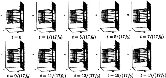
Anumberof sideview

‘snapshots’ ofthe jet during

one

period of the oscillations

are

shown in Fig. 3. The computed

fundamental frequency $f_{0}\approx 190$ Hz, whichis quite close to the experimentally observed value

$ofl96Hz$

.

Figure 3: Side viewofthe jet during

one

period of oscillation.

Velocityfluctionsin the shearlayer

are

illustratedinFig. 4(a). The data have been recorded

0.2

$d_{0}$

away

from the end plate. Part (b) of the figure shows the to part (a) corresponding

fre-quency

spectrum(givenin$dB$

,

using

5

$ms^{-1}$

as

referencevelocity). The level at the characteristic

frequency$f_{0}$isin goodagreement with theexperimentallyrecorded value[11]. The experimental

spectrumcontains however less ‘noise’ and exhibits distinct higherharmonics $(2f_{0},3f_{0}, \ldots)$

.

Figure 4: (a) Velocityfluctuationsin the shear layer at

a

distance0.2$d_{0}$ fromthe endplate. (b)

5

Proper

orthogonal decomposition

analysis

5.1

Description of the method

Proper orthogonal decomposition (POD) is

a

method for extracting coherent structures from

experimental

or

computational data [4]. By coherent

structures

is meant fundamental fluid

modes, containing

a

concentration of vorticity $and/or$ _{responsible for the major part of}

energy

transport.

Thevelocity field$u(x,t)$ _{is recorded at} $N$grid points$x_{1},$$\ldots,x_{N}$ and at $M$ times$t_{1},$

$\ldots,$$t_{M}$

,

$u(x,t)=(\begin{array}{llll}u(x_{l},t_{1}) u(x_{2},t_{l}) u(x_{N},t_{1})u(x_{1},t_{2}) u(x_{2},t_{2}) u(x_{N},t_{2})\vdots \vdots \ddots \vdotsu(x_{1},t_{M}) u(x_{2},t_{m}) u(x_{N},t_{M})\end{array})$

.

(71)

The PODmethod determines

a

set oforthogonal vector functions$\varphi_{n}(x)homA(x, t)$, such that

the expansionof$u(x, t)$ in terms of thesefunctions,‘

$u_{N}(x,t)=\sum_{\mathfrak{n}=1}^{N}a_{\mathfrak{n}}(t)\varphi_{n}(x)$

,

(72)

hasthe smallest error, in the

sense

that

$(||u_{N}-u||^{2}\rangle$ _$arrow\min,$ (73)

where $\Vert\cdot\Vert$ denotes the $L^{2}$-norm, and $\langle\cdot\rangle$ denotes averaging.

The determination ofthePODmodes$\varphi_{\mathfrak{n}}$involves, in the so-calleddirectmethod, thesolution

of

an

$NxN$ eigenvalue problem.

Often the number of grid points $N\gg M$

,

_{the number of temporal points. This is taken}

into advantage in the ‘method ofsnapshots’, where the POD modes $\varphi_{\mathfrak{n}}$

are

written

as a

linear

combination ofthe $Msnap_{8}hots’$,

$\varphi(x)=\sum_{m=1}^{M}c_{m}u(x,t_{m})$

.

(74)

Texts

on

POD,

e.g.

[4], show that the constants $q_{n}$

can

be determined by solving the $MxM$

symmetric eigenvalue problem

$\sum_{m=1}^{M}\frac{1}{M}u_{n}\cdot u_{m}c_{m}=\lambda c_{n}$

,

$n=1,$

$\ldots,$M. (75)

5.2

Numerical

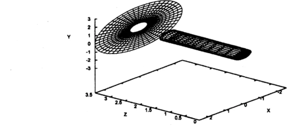
example

Velocities

are

recorded at 51 $x$ 101 grid points,

as

shown in Fig. 5. Snapshots

are

taken

over

10 flow-oscillation periods, with

8

snapshotsin each period. Thus with $N=5151$ and $M=80$,

it is clearly ofadvantageto

use

the method of snapshots. The modal

functions

$\varphi_{1},$

$\ldots,$$\varphi_{4}$

are

shown in Fig.

6..

It should be noted that the

mean

velocity $u_{0}(x)$

was

subtracted before (75)

was

set up and solved. Thus,rather than (72), the expansion

$u_{N}(x,t)=u_{0}(x)+\sum_{n=1}^{N}\tilde{a}_{n}(t)\varphi_{\mathfrak{n}}(x)$ (76)

isconsidered. Mode 1 has

a

mean-flow-like appearance,while modes 2, 3,and 4

are

characterized

Figure

5:

The51$x$

101

gridused for obtainingvelocity snapshots. (a) The wholecomputational

system. (b) Zoom-in aroundthe grid.

that the mentionedphenomenon of modejumpsis related to the mutualbalancebetween these

fundamental

modes. Thiscan,

we

believe, beverifiedby

a

low-dimensionalanalysisbased

on

the

Euler equations, discretized via the

Galerkin

method, with the POD modes

as

basis

functions.

Rowley et al. have applied such

an

approach to the problemofself-sustainedoscillations in the

flow

over

a

rectangular cavity, andfound that the results of

a

full simulation could be captured

bythe Galerkin approximation using justfour modes.

Figure 6: POD modes 1 through 4 (from left to right). The figures in the upper

row

show

velocity vectors; thosein the lower

row

are

iso-velocitycontourplots. Thecoordinates

are as

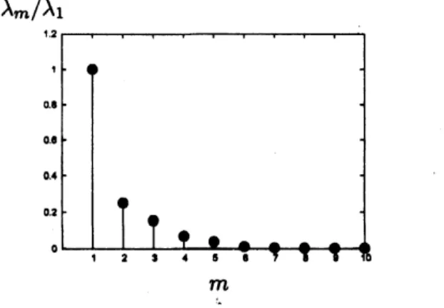
in

This appears to apply to the present problem

as

well. Theeigenvalues $\lambda_{m}$ of (75)

are

shown

inFig.

7.

These eigenvaluev represent twice the kinetic

energy

of the corresponding

mode

$\varphi_{m}$

.

It is

seen

that themagnitudefalls off rapidlywithincreasing mode number. Thusonly thefirst

four

or

five modes will be ofsignificance ingoverning the dynamics ofthe system.

$m$

Figure

7:

Eigenvalues related to the POD modes.

Acknowledgement

The support of the present project through

a JSPS

Grant-in-Aid for Scientific Research (No. 18560152) is gratefully acknowledged.

References

[1] W.T. Ashurst, $E$, Meiburg, Three-dimensional shear layers via vortex dynamics, J. Fluid

Mech.

189

(1988),

87-116.

[2] R.C. Chanaud, A. Powell, Someexperiments concerningthe hole and ring tone, J. Acoust.

Soc. Am. 37 (1965) 902-911.

[3] R.D. Cook, D.S. Malkus, M.E. Plesha, Concepts andApplications

_of

Finite Element

Anal-ysis, John Wiley&Sons, New York,

1989.

[4] P. Holmes, J.L. Lumley, G. Berkooz, $\mathfrak{R}$rbulence, Coherent Structures, Dynamical Systems

and Symmetry, Cambridge University Press, Cambridge UK, 1996.

[5] M. S. Howe, Theory

_of

VortexSound, Cambridge University Press, Cambridge UK,

2003.

[6] J. Katz, A. Plotkin, Low-SpeedAerdynamics,CambridgeUniversity Press, CambridgeUK,

2001.

[7] C. Lanczos, Applied Analysis, DoverPublications, NewYork, 1988.

[8] M.A. Langthjem, M.Nakano, A numericalstudyon the influence of non-axisymmetric flow

perturbations

on

the holetone feedback cycle, RIMS K\^oky\^urvku

1543

(2007),

21-30.

[9] A.Leonard,Computingthree-dimensionalincompressibleflows withvortexelements,Annu.

Rev. Fluid Mech. 17 (1985), 523-559.

[10] P.M. Morse, K.U.Ingard, Theoretical Acoustics, PrincetonUniversity Press, Princeton NJ,

[11] M. Nakano, D. Tsuchidoi, K. Kohiyama, A. Rinoshika, K. Shirono, Wavelet analysis on

behavior of hole-tone self-sustained oscillation of impinging circular air jet subjected to

acousticexcitation, (In Japanese) Kashikajouhou 24 (2004), 87-90.

[12] B. Noble, Methods based on the Wiener-HopfTechnique

_for

the Solution

_of

Partial

Differ-ential Equations, Chelsea Publishing Company, New York, 1988.

[13]

I.G.

Petrovsky, Lectures

on

Partial

_Differential

Equations, Dover Publications, NewYork,

1991.

[14] A. Pikovsky, M. Rosenblum, J. Kurths, Syncronization: A Universal Concept inNonlinear

Sciences, Cambridge University Press, Cambridge UK, 2001.

[15] LordRayleigh, The Theory

_of

Sound, Vol. II, DoverPublications, NewYork,

1945.

[16] Rockwell, D., Naudascher, E., Self-sustained oscillations of impinging

&oe

shear layers.

Annu. Rev. Fluid Mech. 11 (1979)

67-94.

[17] Rockwell, D., Oscillations ofimpinging shear layers. AIAA J. 21 (1983)

645-664.

[18]

C.W.

Rowley, T. Colonius, R.M. Murray, Model reduction for compraesible flows using

POD and

Galerkin

projection, Physica $D$

189

(2004),

115-129.

[19] T. Terai,

On

calculation of sound fields around three dimensional objects by integral