SEMILINEAR ELLIPTIC EQUATIONS WITH CRITICAL SOBOLEV EXPONENT AND NON-HOMOGENEOUS TERM (Shapes and other properties of solutions of PDEs)

全文

(1)1. 数理解析研究所講究録第2006巻 2016年 1-11. SEMILINEAR ELLIPTIC. EQUATIONS WITH CRITICAL SOBOLEV EXPONENT. AND NON‐HOMOGENEOUS TERM KAZUNE TAKAHASHI. 1. INTRODUCTION Let N\geq 3 and a. function. under. zero. discuss the. so. $\Omega$\subset \mathbb{R}^{N} be. a. bounded domain whose. that a\geq K in $\Omega$ for. Dirichlet condition. on. some. boundary. is smooth. Set. constant K>-K_{1} , where K_{1} be the first. $\Omega$ Let .. b\in L^{\infty}( $\Omega$). be. a. a\in L^{\infty}( $\Omega$) be eigenvalue of - $\Delta$. function with b\geq 0 in $\Omega$ and b\not\equiv 0 We .. following equation:. \left{begin{ary}l -$\Delta$u+ =bu^{p}+$\lambd$f&\mathr{i}\mathr{n}$\Omega$,\ u>0&\mathr{i}\mathr{n}$\Omega$,\ u=0&\mathr{o}\mathr{n}\partil$\Omega$. \end{ary}\ight.. ()_{ $\lambda$}. Here, p=(N+2)/(N-2) is the critical Sobolev exponent, and f\in H^{-1}( $\Omega$) is a non‐homogeneous perturbation with f\geq 0 and f\not\equiv 0. $\lambda$>0 is a parameter. This equation is involving the critical Sobolev exponent. It is known the existence and nonexis‐ tence of positive solution depends on the dimension N and the shape of the domain $\Omega$. Let us recall some facts of the Sobolev embedding. Now we assume $\Omega$ is a bounded domain, where the Sobolev space H_{0}^{1}( $\Omega$) is compactly embedded in L^{q}( $\Omega$) for 1\leq q<p+1 The Sobolev space H_{0}^{1}( $\Omega$) is also a subspace of L^{p+1}( $\Omega$) However, it is not compactly embedded. This fact make it difficult to analyze critical equations. Let us recall the definition of a weak solution. u\in H_{0}^{1}( $\Omega$) is a weak solution of ()_{ $\lambda$} if the holds for all : following $\psi$\in H_{0}^{1}( $\Omega$) .. .. \displaystyle \int_{ $\Omega$} (Du . D $\psi$+au $\psi$)dx=\int_{ $\Omega$}bu^{p} $\psi$ dx+ $\lambda$\int_{ $\Omega$}f $\psi$ dx. Here,. we. have to consider the. embedded in. L^{p+1}( $\Omega$) use. .. L^{p+1}( $\Omega$). ,. integral of (p+1) ‐th power of H_{0}^{1} ‐function.. each bounded sequence in. We would have. a. other methods. We find. weak solution. keys. easily.. for the critical. H_{0}^{1}( $\Omega$). would have. But it is not the. equations. case.. a. If. H_{0}^{1}( $\Omega$). compactly convergent subsequence in. To get. in the next section.. were. solutions,. we. have to.

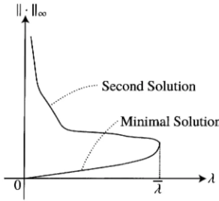
(2) 2. 2. KNOWN RESULTS. AND. MAIN THEOREM. 2.1. Known Results. We recall known results of critical. equations.. Let us. begin with the following. equation:. \left{bginary}{l -$\Delta$u=\lambd$(1+u)^{p}&\mathr{i}\mathr{n}$\Omega$,\ u>0&\mathr{i}\mathr{n}$\Omega$,\ u=0&\mathr{o}\mathr{n}\partil$\Omega$. \end{ary}\ight.. (1) This. equation,. as. well. as. the main. problem,. is. non‐homogeneous. and. we are. interested in. positive. solutions. We introduce two type of solutions. They are called the minimal solution and a second solution. \underline{u}_{$\lambda$} is called the minimal solution if u\geq\underline{u}_{ $\lambda$} in $\Omega$ holds for any solution u We consider .. another solution. \overline{u}_{$\lambda$} other than the minimal solution. For convenience, The facts of the minimal solution of (1) are stated as following:. Theorem 1 ([KK74],. (i) (1) (ii) (1). (iii) (1) has. \overline{$\lambda$} is. [CR75]). 0<\overline{ $\lambda$}<\infty. has the minimal solution \underline{u}_{$\lambda$} for has only one weak solution. exists which. call it. the following. a. second solution.. (i)-(iii). :. 0< $\lambda$<\overline{ $\lambda$}.. \underline{u}_{ $\lambda$-}when $\lambda$=\overline{ $\lambda$}.. no. weak solution for $\lambda$> $\lambda$.. often called the extremal value. The facts of. Theorem 2. There exists This fact. satisfies. we. was. shown. second solution \overline{u}_{$\lambda$} for. a. by Joseph. and. a. second solution. of(1). stated. are. as. following:. 0< $\lambda$<\overline{ $\lambda$} satisfying \overline{u}_{ $\lambda$}\geq\underline{u}_{ $\lambda$}.. Lundgren [JL73]. if $\Omega$. was a. ball.. They. used. radially. ODE. methods. On the other hand, Brézis and Nirenberg [BN83] showed this fact without restriction of $\Omega$ They used two tools, the mountain pass theorem without (PS) condition and the Talenti function. .. Proposition (Mountain pass theorem without (PS) condition [AR73]). Let X be a Banach space. a C^{1} ‐class functional on X. Suppose that there exist a neighborhood U of 0\in X and a constant $\rho$ so that $\Phi$(u)\geq pfor all u\in\partial U Assume that I(0)< $\rho$ and l(v)<pfor some v\in X\backslash U. Let c=\displaystyle \inf_{P\in P}\max_{w\in P}I(w)\geq $\rho$ where \mathcal{P} is the set ofpaths from 0 to v in X. Then, there exists a sequence \{v_{k}\}_{k=0}^{\infty} of X satisfying the following (i) and (ii): (i) \displaystyle \lim_{k\rightarrow\infty}I_{ $\lambda$}(v_{k})=c. Let I be. .. (ii) If. \displaystyle \lim_{k\rightar ow\infty}I_{ $\lambda$}'(v_{k})=0 in X^{*}. we use. the variational method, critical equations, we often need. theorem for critical. points. (\mathrm{P}\mathrm{S})_{c}. are. solutions of the. condition instead of. Definition. Let X be. (\mathrm{P}\mathrm{S})_{c} a. equation. To apply (PS) condition.. this. a Banach space. Let I be a functional on X Let c\in \mathbb{R} We say I satisfies condition if any sequence \{v_{k}\}_{k=0}^{\infty} of X satisfying (i) and (ii) stated in Proposition above has .. .. convergent subsequence.. Broadly speaking,. in. our. of noncompact sequences.. case, if the. Actually,. highest point c is not. so. high,. we can. rule out the. possibility. it is related to the Talenti function. We discuss it in the next. section. We summarize solutions of. vertical axis. we. would have. (1) by using diagrams (Figure 1). On the horizontal axis is $\lambda$ On the if we could. Of course, H_{0}^{1}( $\Omega$) is infinitely dimensional. We. H_{0}^{1}( $\Omega$). ,.

(3) 3. use. the L^{\infty} ‐norm instead of that. If. cross. at two. That. points.. starts at 0 and ends at. means we. $\lambda$=\overline{ $\lambda$}. .. The. we. fix. a. have two. $\lambda$>0. ,. we. positive. find that the vertical line and the. solutions. The. curve. diagram. of the minimal solution. increases. It means the bigger $\lambda$ is, the bigger L^{\infty} ‐norm actually proved. The curve of the second solution starts at $\lambda$=\overline{ $\lambda$} (1) has only one solution. curve. of the minimal solution is. This fact is. $\lambda$=\overline{ $\lambda$} and. goes. reversely.. FIGURE 1. The. When. diagram. ,. of solutions of (1).. On the horizontal axis is $\lambda$. .. On the. vertical axis is L^{\infty} ‐norm. The branch of the minimal solution starts from 0 and ends at. $\lambda$=\overline{ $\lambda$}. .. The branch of. a. second solution starts from that end. point and goes. reversely. The mountain pass theorem without. (PS) condition and the Talenti function. are. efficient for. our. types. The following equation is the main problem ()_{ $\lambda$} with a=0 and b=1 :. \left{bginary}{l -$\Deltau=^{p}+$\lambd$f&\mathr{i}\mathr{n}$\Omega$,\ u>0&\mathr{i}\mathr{n}$\Omega$,\ u=0&\mathr{o}\mathr{n}\partil$\Omega$. \end{ary}\ight.. (2). Tarantello [Tar92] proved that it has two positive solutions for sufficiently small $\lambda$>0. The following equation is the main problem ()_{ $\lambda$} with a be a constant K and b=1 :. \left{begin{ary}l -$\Delta$u+K=^{p}+$\lambd$f&\mathr{i}\mathr{n}$\Omega$\ u>0&\mathr{i}\mathr{n}$\Omega$,\ u=0&\mathr{o}\mathr{n}\partil$\Omega$. \end{ary}\ight.. (3) It has. a. linear term of. minimal solution. are. the second solutions. Theorem 3. Naito and Sato. [NS12] investigated this equation. The results of the way as Theorem 1. On the other hand, the results of different from (1) and (2).. u. .. summarized in the are. ([NS12] Theorem 1.3).. Let. same. 0< $\lambda$<\overline{ $\lambda$}. .. Assume that either. and N\geq 3.. (i) -K_{1}<K\leq 0 (ii) K>0 and N=3 4, 5. ,. Then, (3) has. a. second solution. \overline{u}_{ $\lambda$}\in H_{0}^{1}( $\Omega$) satisfying \overline{u}_{$\lambda$}>\underline{u}_{$\lambda$}. in $\Omega$.. (i). or. (ii) holds..

(4) 4. Naito and Sato also. proved that, if K>0 and N\geq 6 there is a case the equation has only one sufficiently small $\lambda$>0 In this sense, the statement of (ii) gives the best result. We use the diagrams to view these results (Figure. 2). Let K>0 If N=3 4, 5, the branch of a second solution is approaching to the extent of $\lambda$=0 However, if N\geq 6 the climate changes. The branch of second solution cannot go beyond some positive $\lambda$. ,. solution for. .. .. ,. .. ,. FIGURE 2. The. If N=3. ,. diagram of solutions of(3) depends on the dimension N when K>0. 4, 5, the branch of a second solution is approaching to the extent of $\lambda$=0. like the left like the. figure, while right figure.. 2.2. Main Theorem. Now. we. if N\geq 6 there is. a case. ,. consider the main. that it cannot go. problem ()_{ $\lambda$}. .. First. we. beyond. some. $\lambda$. state the results of the. minimal solution. Theorem 4. (i) (1) (ii) (1). ([Tak15]. Theorem 1.1,. 1.2). 0<\overline{ $\lambda$}<\infty. has the minimal solution \underline{u}_{$\lambda$} for has only one weak solution. (iii) (1) has. no. exists which. when. the following. (i)-(iii). :. \underline{u}_{ $\lambda$}when $\lambda$-=\overline{ $\lambda$} if b>0 in $\Omega$.. weak solution for $\lambda$> $\lambda$.. The main result of the minimal solution is almost the occurs. satisfies. 0< $\lambda$<\overline{ $\lambda$}.. $\lambda$=\overline{ $\lambda$}. .. Since b is. a. function,. we assume. same as. Theorem 1. A miner difference. b>0 in $\Omega$ to get the. uniqueness of the. solution. Now. we. state the main result.. ([Tak15] Theorem 1.4). Let 0< $\lambda$<\overline{ $\lambda$} M=1b||_{L^{\infty}( $\Omega$)}>0 at a point x_{0} in $\Omega$ Suppose that there b is continuous in \{|x-x_{0}|<r_{0}\} and Theorem 5. .. .. Suppose exists. that b achieves its maximum. r_{0}>0 so that \{|x-x_{0}|<2r_{0}\}\subset $\Omega$,. ,. a(x)=m_{1}+m_{2}|x-x_{0}|^{q}+o(|x-x_{0}|^{q}) Here, q>0, m_{1}>K and m_{2}\neq 0 ,. and N\geq 3.. (i) m_{1}<0 (ii) m_{1}>0 and N=3 4, 5. (iii) m_{1}=0, m_{2}<0 and N\geq 3. ,. are. constants.. in. \{|x-x_{0}|<r_{0}\}.. Assume that either. (i)-(iv) holds..

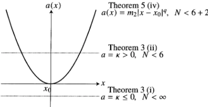
(5) 5. (iv) m_{1}=0, m_{2}>0 Then, ()_{ $\lambda$} has. a. and. 3\leq N<6+2q.. second solution. \overline{u}_{ $\lambda$}\in H_{0}^{1}( $\Omega$) satisfying \overline{u}_{$\lambda$}>\underline{u}_{$\lambda$}. The main theorem gives sufficient conditions where. have two solutions for 0< $\lambda$<\overline{ $\lambda$}. we. .. Though. like Naito and Satos results, (iv) seems to be new. In (iv), we have two solutions if N<6+2q This occurs since coefficients a and b are functions on $\Omega$.. (\mathrm{i})-(\mathrm{i}\mathrm{i}\mathrm{i}). 3\leq. in $\Omega$.. are. .. We compare (3) and the main problem ()_{ $\lambda$} We focus on the dimension where there exists a second solution for any 0< $\lambda$< $\lambda$ In Theorem 3 (i) and (ii), when K stride across zero, the upper bound of the dimension jumps from \infty to 6. We consider this result from the main problem ()_{ $\lambda$}. .. .. Theorem 3 is. regarded as the case that a is a constant K On the other hand, in the main problem ()_{ $\lambda$}, a is a function. We can think of a function whose order is q at x_{0} which appears in Theorem 5 (iv). In this case, the upper bound of the dimension is 6+2q Therefore, this can be regarded as a intermediate case of Naito and Satos results (Figure 3). .. ,. .. FIGURE 3. The dimension where. ()_{ $\lambda$} has a second solution varies depending on the a(x) Theorem 5 (iv), in which a increases in order q around zero point x_{0}, can be interpreted as a intermediate case between Theorem 3 (i) and (ii), in which a function is. a. .. constant. K.. 3. PROOF. 0F. MAIN THEOREM. We. move on to the summary of the proof of Theorem 5. We start at the point that we already investigated the minimal solution \underline{u}_{$\lambda$} of ()_{ $\lambda$} We assume 0< $\lambda$<\overline{ $\lambda$} We can also assume that x_{0}=0 by translation of axes if we need. We are now interested in the second solutions. Instead of chasing a second solution directly, we consider the difference between a second solution \overline{u}_{$\lambda$} and the minimal solution \underline{u}_{$\lambda$} We name it v=\overline{u}_{ $\lambda$}-\underline{u}_{ $\lambda$} which satisfies the following:. have. .. .. (v). ,. \left{begin{ary}l -$\Delta$v+ =b(v+\underli {u}_$\lambd$})^{p-\underli {u}_$\lambd$}^{p)&\mathr{i}\mathr{n}$\Omega$,\ v>0&\mathr{i}\mathr{n}$\Omega$,\ v=0&\mathr{o}\mathr{n}\partil$\Omega$. \end{ary}\ight.. ..

(6) 6. The main. has. problem ()_{ $\lambda$}. a. second solution if and. only. if. (\nabla)_{ $\lambda$} has. a. solution. It follows that. v>0 in $\Omega$ because of the definition of the minimal solution and the strong maximum principle. We use the variational method to prove the existence of v We define a functional I_{ $\lambda$} as following: .. I_{ $\lambda$}(v)=\displaystyle \frac{1}{2}\int_{ $\Omega$}|Dv|^{2}dx-\int_{ $\Omega$}G(v,\underline{u}_{ $\lambda$})dx,. (4) where. g(t, s, x)=b(x)((t_{+}+s)^{p}-s^{p})-a(x)t_{+},. (5). G(t, s, x)=\displaystyle \int_{0}^{f_{+} g(t, s, x)dt =b(x)(\displaystyle \frac{1}{p+1}(t_{+}+s)^{p+1}-\frac{1}{p+1}s^{p+1}-s^{p}t_{+})-\frac{1}{2}a(x)t_{+}^{2},. (6) and we. we. get. write a. g(v,\underline{u}_{ $\lambda$}). solution of. as. g(v,\underline{u}_{ $\lambda$}, x). (\wp)_{ $\lambda$}. .. It. and. means. G(v, \underline{u}_{ $\lambda$}). that. we. get. as a. G(v,\underline{u}_{ $\lambda$}, x). If. .. second solution. find. we. \overline{u}_{$\lambda$}. as. a. critical. the. sum. point. v. of I_{ $\lambda$},. of the minimal. solution \underline{u}_{$\lambda$} and the critical point v. We combine the mountain pass theorem and the Talenti function.. Through a. argument,. some. function. v_{0}\in H_{0}^{1}( $\Omega$). so. we can. that. find. v_{0}\geq 0. a. We need (PS)_{c} condition. (PS)_{c} condition, that is, there exists. in $\Omega$ and. \displaystyle \int_{ $\Omega$}bv_{0}^{p+1}dx>0,. (7) and. \displaystyle\sup_{t>0}I_{$\lambda$} (tvo) <\displaystyle \frac{1}{NM^{(N-2)/2} S^{N/2}.. (8). Here, M is the maximum value of b. constant S is defined. S=. V\subset \mathbb{R}^{N}. where. achieved ,. by. is. a. S is called the best Sobolev constant.. inf. | Du||_{L^{2}(V)}^{2}. u\in H_{0}^{1}(V),u\not\equiv 0\overline{| u| _{L^{p+1}(V)}^{2}. domain. It is known that S does not. the Tarenti function. This fact is. we use. important. . depend. when. we. the Talenti function. The Talenti function U is. on. V. .. This infimum is. (11). (8).. We define u_{ $\epsilon$} and v_{ $\epsilon$}. given. u_{ $\epsilon$}(x)=\displaystyle \frac{ $\eta$(x)}{( $\epsilon$+|x^{2})^{(N-2)/2} ,. as. v_{$\epsilon$}(x)=\displaystyle\frac{u_{$\epsilon$}(x)}{\Vertb^{1/(p+1)}u_{$\epsilon$}|_{L^{p+1}($\Omega$)}.. actually. compute the condition (8). To get as. following:. U(x)=\displaystyle \frac{1}{(1+|x|^{2})^{(N-2)/2} . Our aim is to get v_{0} of the condition. (10). The best Sobolev. by following:. (9). this v_{0}. sufficient condition of. following:.

(7) 7. Here, $\epsilon$>0 and in. case. (i). $\eta$ is. (iii),. or. a. cut‐off function around O. v_{ $\epsilon$} is some kind of normalization of u_{ $\epsilon$} Note change r_{0}>0 for smaller one if we need so that .. \displaystyle\int_{$\Omega$}av_{$\epsilon$}^{2}dx\leq0.. (12) Note also. that,. in. case. (ii). or. (iv),. we can. change r_{0}>0. for smaller. one. if we need. so. that. \displaystyle\int_{$\Omega$}av_{$\epsilon$}^{2}dx\geq0.. (13) Now. we. compute the condition (8). Through. achieved at. actually. Then,. that,. we can. we. some. positive t=t_{ $\epsilon$} We .. argument, We. some. are. going. to estimate. can see. I_{ $\lambda$}(t_{ $\epsilon$}v_{ $\epsilon$}). .. the supremum in We define. (8). is. H'(v,\displaystyle \underline{u}_{ $\lambda$})=\frac{1}{p+1}(v+\underline{u}_{ $\lambda$})^{p+1}-\frac{1}{p+1}v^{p+1}-\frac{1}{p+1}\underline{u}_{ $\lambda$}^{p+1}-\underline{u}_{ $\lambda$}^{p}v.. have. \displaystyle \sup_{t>0}I_{ $\lambda$}(tv_{ $\epsilon$})=I_{ $\lambda$}(t_{ $\epsilon$}v_{ $\epsilon$}). =\displaystyle\frac{1}{2}t_{$\epsilon$}^{2}|v_{$\epsilon$}|^{2}-\frac{1}{p+1}t_{$\epsilon$}^{p+1}-\int_{$\Omega$}H'(t_{$\epsilon$}v_{$\epsilon$},\underline{u}_{$\lambda$})dx+t_{$\epsilon$}^{2}\int_{$\Omega$}av_{$\epsilon$}^{2}dx,. (14) where. The term. containing. divide the. proof into. For. case. (i). and. a. is. |v_{$\epsilon$}|=(\displaystyle\int_{$\Omega$}|Dv_{$\epsilon$}|^{2}dx)^{1/2}. important for this argument.. The. $\epsilon$ ‐order. of that term. depends. on. q. .. We. two cases.. (iii), by (12),. we. have. \displaystyle\sup_{t>0}I_{$\lambda$}(tv_{$\epsilon$})\leq\frac{1}{2}t_{$\epsilon$}^{2}|v_{$\epsilon$}|^{2}-\frac{1}{p+1}t_{$\epsilon$}^{p+1}-\int_{$\Omega$}H'(t_{$\epsilon$}v_{$\epsilon$},\underline{u}_{$\lambda$})dx. \displaystyle \leq\sup_{t>0}(\frac{1}{2}t^{2}|v_{ $\epsilon$}|^{2}-\frac{1}{p+1}t^{p+1})-\int_{ $\Omega$}H'(t_{ $\epsilon$}v_{ $\epsilon$}, \underline{u}_{ $\lambda$})dx. =\displaystyle\frac{1}{N}(|v_{$\epsilon$}|^{2})^{N/2}-\int_{$\Omega$}H'(t_{$\epsilon$}v_{$\epsilon$},\underline{u}_{$\lambda$})dx. By calculation,. we. have. |v_{ $\epsilon$}|^{2}=\displaystyle \Vert Dv_{ $\epsilon$}|_{L^{2}( $\Omega$)}^{2}=\frac{S}{M^{2/(p+1)} +O($\epsilon$^{(N-2)/2}). (15) as. $\epsilon$\searrow 0 that is,. as. $\epsilon$\searrow 0. ,. .. there exist. (16). \displaystyle \frac{1}{N}(| v_{ $\epsilon$}| ^{2})^{N/2}=\frac{1}{NM^{(N-2)/2} S^{N/2}+O($\epsilon$^{(N-2)/2}). H', (p+1) ‐th powered terms are canceled. After some argument, $\epsilon$_{0}>0 and C>0 so that for all 0< $\epsilon$<$\epsilon$_{0} the following holds: In. ,. \displaystyle\int_{$\Omega$}H'(t_{$\epsilon$}v_{$\epsilon$},\underline{u}_{$\lambda$})dx\geqC$\epsilon$^{(N-2)/4}.. we can. show that.

(8) 8. Summing. up these results, there exist. $\epsilon$_{0}>0 and C, C'>0. so. that for all. 0< $\epsilon$<$\epsilon$_{0}. \displaystyle \sup_{t>0}I_{ $\lambda$}(tv_{ $\epsilon$})\leq\frac{1}{NM^{(N-2)/2} S^{N/2}+(C$\epsilon$^{(N-2)/2}-C'$\epsilon$^{(N-2)/4}). (17). ,. we. have. .. For any N\geq 3 it holds that (N-2)/2>(N-2)/4 Thus there exists $\epsilon$>0 so that the terms in of the right side of (17) is negative. If we use this $\epsilon$ for v_{0}=v_{ $\epsilon$}, v_{0}\geq 0 in $\Omega$ (7), and ,. .. parentheses (8). are. For. ,. all satisfied. Thus case. (ii). and. we. have. (iv), by (12),. a. we. second solution of. ()_{ $\lambda$}.. have. \displaystyle\sup_{t>0}I_{$\lambda$}(tv_{$\epsilon$})=\frac{1}{2}t_{$\epsilon$}^{2}(|v_{$\epsilon$}|^{2}+2\int_{$\Omega$}av_{$\epsilon$}^{2}dx)-\frac{1}{p+1}t_{$\epsilon$}^{p+1}-\int_{$\Omega$}H'(t_{$\epsilon$}v_{$\epsilon$},\underline{u}_{$\lambda$})dx \displaystyle \leq\sup_{t>0}(\frac{1}{2}t^{2}(|v_{ $\epsilon$}|^{2}+2\int_{ $\Omega$}av_{ $\epsilon$}^{2}dx)-\frac{1}{p+1}t^{p+1})-\int_{ $\Omega$}H'(t_{ $\epsilon$}v_{ $\epsilon$}, \underline{u}_{ $\lambda$})dx. =\displaystyle\frac{1}{N}(|v_{$\epsilon$}|^{2}+2\int_{$\Omega$}av_{$\epsilon$}^{2}dx)^{N/2}-\int_{$\Omega$}H'(t_{$\epsilon$}v_{$\epsilon$},\underline{u}_{$\lambda$})dx.. Here. we. define. A( $\epsilon$). as. following:. A( $\epsilon$)=\displaystyle \frac{1}{N}(|v_{ $\epsilon$}|^{2}+2\int_{ $\Omega$}av_{ $\epsilon$}^{2}dx)^{N/2}-\frac{1}{NM^{(N-2)/2} S^{N/2}. We. are now. at the. point to evaluate the integral of av_{ $\epsilon$}^{2}. .. We define. I_{1}=\displaystyle \int_{\{|x<r_{0}\} \frac{1}{( $\epsilon$+|x^{2})^{N-2} dx, I_{2}=\displaystyle \int_{\{|x<r_{0}\} \frac{|x^{q} {( $\epsilon$+|x^{2})^{N-2} dx. The estimate of I_{1} is famous.. other. I_{2} is. evaluate I_{2}.. To. Many paper refers to Brézis‐Nirenberg [BN83]. On the Brézis‐Nirenberg. We use almost the same method of Brézis‐Nirenberg to describe only the results, we have the following: not on. (18). We. can. (19). also evaluate. \left\{ begin{ar y}{l I_{1}=[Case]\ I_{2}=[Case] \end{ar y}\right. \Vert b^{1/(p+1)}u_{ $\epsilon$}\Vert_{L^{p+1}( $\Omega$)}^{2}=O($\epsilon$^{-(N-2)/2}). hand,.

(9) 9. $\epsilon$\searrow 0 Therefore,. as. .. admit the. we. following:. \left{bginary}{l \int_$Omega}v_{$\epsilon}^{2dx=O($\epsilon^{(N-2)/}+m_{1I}'+m_{2I}',\ _{1=[Case](N3=4\geq5 I_{2}'=[Case] \nd{ary}\ight.. (20). $\epsilon$\searrow 0 We can see I_{2}' is affected with q Note that, for all case, I_{i}'\gg$\epsilon$^{(N-2)/2} or I_{i}'=O($\epsilon$^{(N-2)/2}) $\epsilon$\searrow 0 for i=1 2. Note also that I_{1}\gg I_{2} as $\epsilon$\searrow 0 for any N\geq 3, q>0 Considering (15) and (20), we have the evaluation of A( $\epsilon$) as following: as. .. .. as. ,. $\Lambd(epsilon$)=\ft{beginary}l O($\epsion)&(m_{1}>0,N\geq5) O($\epsilon|g$\epsilon|)&(m_{1}>0,N=4)\ O($epsilon^{1/2})&(m_>0,N=3)\ O($epsilon^{1+q/2})&(m_{1=0, 2}>Nq+4),\ O($epsilon^{N-2)/}|\log$epsin|)&(m_{1}=0, 2>N=q+4),\ O($epsilon^{N-2)/}&(m_{1=0, 2}>N<q+4) \end{ary}ight.. (21). as. $\epsilon$\searrow 0 By (16), there .. we. of. (22). exist. $\epsilon$_{0}>0 and C'>0. so. that for all 0< $\epsilon$<$\epsilon$_{0},. \displaystyle \sup_{t>0}I_{ $\lambda$}(tv_{ $\epsilon$})\leq\frac{1}{NM^{(N-2)/2} S^{N/2}+(A( $\epsilon$)-C'$\epsilon$^{(N-2)/4}). (22) As. .. .. discussed. before, if there exists $\epsilon$>0 so that the terms in parentheses of the right side negative, we have a second solution of ()_{ $\lambda$} If m_{1}>0 and N=3 4, 5, it holds that A( $\epsilon$)\ll$\epsilon$^{(N-2)/4} as $\epsilon$\searrow 0 by (21). Thus we have the desired $\epsilon$ If m_{1}=0, m_{2}>0 and N\leq q+4, it holds that $\Lambda$( $\epsilon$)\ll$\epsilon$^{(N-2)/4} as $\epsilon$\searrow 0 by (21). If m_{1}=0, m_{2}>0 and N>q+4 the condition where A( $\epsilon$)\ll$\epsilon$^{(N-2)/4} as $\epsilon$\searrow 0 is that 1+q/2>(N-2)/4 Then we have N<2q+6 That is, if m_{1}=0, m_{2}>0 and 3\leq N<2q+6 we have the desired $\epsilon$. In [Tak15] and the talk of this workshop, the author mistakenly dropped t_{ $\epsilon$}^{2} of the last term in (14). The proof should be replaced as above. is. .. ,. .. ,. .. .. ,. AppENDIx A. PROOF. 0F. BOUNDEDNESS \mathrm{o}\mathrm{p} $\lambda$. In the workshop, several people asked the author about the proof of Theorem appendix, we see the summary of that proof. To prove Theorem 4 (iii), we define. \overline{ $\lambda$}= { $\lambda$\geq 0| and. we. show. \overline{ $\lambda$}<\infty. .. The. The main. problem ()_{ $\lambda$}. following argument is. almost the. has. a. 4. (iii).. In this. solution.}. same as. the. proof appeared in [NS12]..

(10) 10. We define. g_{0}\in H_{0}^{1}( $\Omega$). as. the. unique. following equation:. \left\{ begin{ar y}{l -$\Delta$g_{0}+ag_{0}=f\mathrm{i}\mathrm{n}$\Omega$,\ g_{0}= \mathrm{o}\mathrm{n}\parti l$\Omega$. \end{ar y}\right.. (23) We have. solution of the. in $\Omega$. the strong maximum. g_{0}>0 by eigenvalue problem:. principle.. Next. consider the. we. - $\Delta \phi$+a $\phi$= $\mu$ b(g_{0})^{p-1} $\phi$ in $\Omega$, $\phi$\in H_{0}^{1}( $\Omega$). (24) It is known that the first. eigenvalue. (25). $\mu$_{1}=. It is also known that if. (24). Through $\phi$_{1}>0 in $\Omega$.. some. We fix $\lambda$>0. of the main. so. $\mu$_{1} is characterized. inf. that there exists. problem ()_{ $\lambda$}. a. set. right. we. linearized. .. Rayleigh quotient:. $\psi$\inH_{0^{($\Omega$),$\psi$\not\equiv0}\overline{\int_{$\Omega$}b(g_{0})^{p-1}$\psi$^{2}dx} ^{1}. $\phi$ argument we have $\mu$_{1}>0 and. we. the. \displaystyle \int_{ $\Omega$}(|D $\psi$|^{2}+a$\psi$^{2})dx. achieves the infimum of the. and. by. following. side of. find the first. .. (25), $\phi$ is a first eigenfunction of eigenfunction $\phi$_{1} which satisfies. solution of the main. problem ()_{ $\lambda$} v=u- $\lambda$ g_{0} which satisfies. .. We write. u as a. solution. ,. - $\Delta$ v+av=bu^{p}\geq 0. Then we. we. have v>0 in $\Omega$. by the strong maximum principle.. It. that. u> $\lambda$ g_{0}. in $\Omega$. right. side of. (28). means. .. Therefore. get the following:. - $\Delta$ u+au\geq bu^{p}>b$\lambda$^{p-1}(g_{0})^{p-1}u\mathrm{i}\mathrm{n} $\Omega$.. (26) On the other hand,. we. have the. following:. - $\Delta \phi$_{1}+a$\phi$_{1}=$\mu$_{1}b(g_{0})^{p-1}$\phi$_{1}. (27). Integrating (26) \times$\phi$_{1}-(27)\times u. on. $\Omega$. ,. we. admit the. in $\Omega$.. following:. 0>($\lambda$^{p-1}-$\mu$_{1})\displaystyle \int_{ $\Omega$}b(g_{0})^{p-1}u$\phi$_{1}dx.. (28). Since b\geq 0 in $\Omega$, b\not\equiv 0 and g_{0}, u, $\phi$_{1}>0 in $\Omega$ the which implies $\lambda$^{p-1}-$\mu$_{1}<0 Thus we conclude that ,. ,. .. integral. of the. \overline{ $\lambda$}\leq$\mu$_{1}^{1/(p-1)}<\infty.. is. positive,. REFERENCES. [AR73]. Antonio Ambrosetti and Paul H. Rabinowitz. Dual variational methods in critical point theory and applications.. J. FunctionalAnalysis, 14:349−381 1973. [BN83] Haim Brézis and Louis Nirenberg. Positive solutions of nonlinear elliptic equations involving critical Sobolev exponents. Comm. Pure Appl. Math., 36(4):437-477 1983. [CR75] Michael G. Crandall and Paul H. Rabinowitz. Some continuation and variational methods for positive solutions of nonlinear elliptic eigenvalue problems. Arch. Rational Mech. Anal. 58(3):207-218 1975. [L73] Daniel D. Joseph and Thomas S. Lundgren. Quasilinear Dirichlet problems driven by positive sources. Arch. Rational Mech. Anal. 49:241−269, 1972/73. [KK74] James P. Keener and Herbert B. Keller. Positive solutions of convex nonlinear eigenvalue problems. J. Differ‐ ential Equations, 16: 103‐125, 1974. ,. ,. ,. ,. ,.

(11) 11. [NS12] Yuki Naito and Tokushi Sato. Non‐homogeneous semilinear elliptic equations involving critical Sobolev exponent. Ann. Mat. Pura Appl. (4), 191(1):25−51 2012. [Tak15] Kazune Takahashi. Semilinear elliptic equations with critical sobolev exponent and non‐homogeneous term. Master thesis, The University of Tokyo. 2015. [Tar92] Gabriella Tarantello. On nonhomogeneous elliptic equations involving critical Sobolev exponent. Ann. Inst. H Poincaré Anal. Non Linéaire, 9(3):281‐304, 1992. ,. ,. (K. Takahashi) GRADUATE SCHOOL. OF. MATHEMATTCAL SCTENCES, THE UNIVERSITY. MEGUROKU ToKyo 153‐8914, JAPAN E‐mail address: [email protected]‐tokyo.ac.jp. 0F. ToKyo.. 3−8−1 KOMABA.

(12)