On an extension of the $\omega$-subdivision rule used in the simplicial algorithm for convex maximization (The state-of-the-art optimization technique and future development)

全文

(1)167. 数理解析研究所講究録第2027巻 2017年 167-178. On in the. an. extension of the. $\omega$ ‐subdivision. rule used. simplicial algorithm for convex maximization Takahito Kuno. *. Graduate School of Systems and Information. University. Engineering. of Tsukuba, Tsukuba, Ibaraki 305‐8573,. Japan.. Abstract In this paper,. plementing. we. discuss. under the. process and extend. difficulties of the. some. $\omega$ ‐subdivision. $\omega$ ‐subdivision.. algorithm according to. this. new. We also. simplicial algorithm detected in im‐ those, we modify the bounding numerical results for the simplicial report overcome. subdivision rule.. Key words: Global optimization, algorithm, a)‐subdivision. 1. rule. To. convex. maximization, branch‐and‐bound, simplicial. Introduction. In 1976, Horst proposed a kind of branch‐and‐bound algorithm, named the simplicial algo‐ rithm, to solve convex maximization problems [3]. The algorithm now counted among the. popular algorithms in global optimization [4, 5, 14], along with the conical algorithm proposed by Tuy in 1964 [17]. In the branching process, whereas the latter uses cones, the simplicial algorithm uses a set of simplices to partition the feasible set; and in the bounding process, the algorithm estimates an upper bound of the objective function by maximizing its convex envelope on each simplex, which is further subdivided to refine the partition if the bound is for As a rule Horst used a one which bisects subdivision, upper large enough. simple each simplex across its longest edge, and gave a convergence proof for the algorithm. Al‐ though his proof contains a flaw, Thoai‐Tuy [16] found and fixed it later, and also introduced most. the concept of exhaustiveness as a sufficient condition for the convergence. On the other hand, in the conical algorithm, Tuy utilized a byproduct of the bounding process to subdivide each. without a guarantee of convergence. Even for the simplicial algorithm, we can adopt a similar rule, which subdivides each simplex radially around the maximum point of the con‐. cone. cave envelope obtained as a byproduct in the bounding process. This so‐called $\omega$ ‐subdivision rule is not exhaustive, and the convergence of both algorithms incorporating the mle remained open until Jaumard‐Meyer [6] and Locatelli [11] proved it for the conical algorithm indepen‐. dently *. in 1998, 1999, and Locatelli‐RaUer [12, 13] did for the. The author. Society. was. partially supported by. a. for the Promotion of Sciences. \mathrm{E}‐mail:. simplicial algorithm. Grant‐in‐Aid for Scientific Research. takahito@cs.tsukuba.ac.jp. in 2000.. (C) 16\mathrm{K}00028 from Japan.

(2) 168. Preceding their proofs by nearly. decade, Tuy showed in [18] that the conical algorithm with. a. $\omega$ ‐subdivision. Ishihama. [9]. Kuno‐ converges if a certain nondegeneracy condition holds (see also [5, 19 showed that a more moderate condition always holds and guarantees the conver‐. gence for the conical. algorithm.. In. a. similar way, Kuno‐Uuckland [8] and Kuno‐Ishihama [10]. proved the convergence of the simplicial algorithm and generalized the $\omega$ ‐subdivision rule. In this paper, we discuss some difficulties of the simplicial algorithm detected in imple‐ menting. under the. and extend the. problem. $\omega$ ‐subdivision. $\omega$ ‐subdivision. rule. To. and outline the usual. those,. we modify the bounding process define the target concave maximization for solving it. In Sections 3, we point out. overcome. rule. In Section 2,. we. simplicial algorithm algorithm and propose a technical solution. To cope with some emerging issues, in Section 4, we develop a new simplicial subdivision rule. Lastly, in Section 5, we report numerical results for the simplicial algorithm according to this rule. the difficulties of the. 2. Convex maximization and the. f be a convex polyhedron: Let. simplicial algorithm. function defined. on. \mathbb{R}^{n}. ,. and consider. maximize. f(\mathrm{x}). subject to. Ax. .. and. \mathrm{v}_{1}^{1}. ,. \cdots. (1). Ax \leq \mathrm{b} },. (2). assume. that. an n. ‐simplex S^{1}\subseteq \mathbb{R}^{n}. with. \mathrm{v}_{n+1}^{1}. D\subseteq S^{1}\subset \mathrm{i}\mathrm{n}\mathrm{t}( domf) where \mathrm{d}\mathrm{o}\mathrm{m}. on a. by. that D is nonempty and bounded. We also is given and satisfies ,. assume. vertices. { \mathrm{x}\in \mathbb{R}^{n}|. problem of maximizing it. \leq \mathrm{b},. where \mathrm{A}\in \mathbb{R}^{m\times n} and \mathrm{b}\in \mathbb{R}^{m} Denote the feasible set D=. a. (3). ,. and int represent the effective domain and the interior, respectively. Under these assumptions, (1) has at least one globally optimal solution \mathrm{x}^{*}\in D In general, however, there .. \cdot. .. are. multiple locally optimal solutions, many of which. rigorously,. need to enumerate them. are. not. such. globally optimal. as. To solve. (1). branch‐and‐bound. One of. using techniques standard branch‐and‐Uound approaches is the simplicial algorithm proposed by we. Horst in 1976. [3], outlined below. OUTLINE. OF THE SIMPLICIAL ALGORITHM. As in other branch‐and‐Uound. approaches, the following two processes play major roles in the. simplicial algorithm. Branching: Starting from i=1 the n ‐simplex S^{i}=\mathrm{c}\mathrm{o}\mathrm{n}\mathrm{v}\{\mathrm{v}_{1}^{i}, \cdots, \mathrm{v}_{n+1}^{i}\} ally around a point \mathrm{u}\in S^{i}\backslash \{\mathrm{v}_{1}^{i}, \cdots,\mathrm{v}_{n+1}^{i}\} into at most n+1 children: ,. S_{j}^{i}=\mathrm{c}\mathrm{o}\mathrm{n}\mathrm{v}\{\mathrm{v}_{1}^{i}, \cdots, \mathrm{v}_{j-1}^{i},\mathrm{u},\mathrm{v}_{j+1}^{i}, \mathrm{v}_{n+1}^{i}\}, j\in J^{i}. ,. is subdivided radi‐. (4).

(3) 169. J^{i}. where. is. an. index set such that. j\in J^{i}. dent. Out of active descendants of S^{1} same. process is. contain. no. after. if \mathrm{v}_{1} ,. \cdots. ,. is chosen. simplex incrementing i by. repeated optimal solution of(1).. ,. \mathrm{v}_{j-1}^{i},\mathrm{u},\mathrm{v}_{j+1}^{i}. a. We refer to. as. ,. \cdots. the. ,. \mathrm{v}_{n+1}^{i}. affinely indepen‐ S^{i+1} to S^{i} and the. are. successor. ,. one, until all active descendants turn out to. \mathrm{u} as. the central pointfor subdivision of S^{i}.. Except in the trivial case where D\cap S^{i}=\emptyset whether or not S^{i} needs to be subdi‐ vided is determined by comparing an upper bound $\beta$ of f on D\cap S^{i} with the value $\alpha$ of f at the best known feasible solution. The value of $\beta$ is given by maximizing the concave envelope g^{i} of f the pointwise infimum over all concave overestimators of f on S^{i} In our case where f is a convex function, g^{i} is an affine function which agrees with f at the vertices of S^{i} and Bounding:. ,. ,. .. ,. point \mathrm{t}\mathrm{u}^{i} over D\cap S^{i} can be obtained by linear programming. If $\alpha$\geq $\beta$ then S^{i} contains no feasible solution of value better than $\alpha$ and can be pruned. hence its maximum. for. $\beta$=g^{i}(\mathrm{O}^{j}). ,. from the set of active descendants of If the. algorithm simplices:. nested. S^{1}. which need to be further examined.. does not terminate in. a. finite amount of time, it generates. a. sequence of. S^{1}=S^{i_{1}}\supset\cdots\supset S^{i_{k}}\supset S^{i_{k+1}}\supset\cdots,. S^{i_{k+1}}. is a child of S^{i_{k}} created by subdividing S^{i_{k} around some \mathrm{u}\in S^{i_{k} The convergence algorithm depends largely on how to subdivide S^{i} in the branching process. If \mathrm{u} is placed at the midpoint on a longest edge of S^{i} for each i then S^{i_{k} shrinks to a single point as k\rightarrow\infty Since t1^{i_{k}} belongs to S^{i_{k} we simultaneously have. where. .. of the. ,. .. ,. \displaystyle \lim_{k\rightar ow}\inf_{\infty}(g^{i_{k} (\mathrm{m}^{i_{k} )-f(\mathrm{m}^{i_{k} ) =0. *. This guarantees the convergence of the algorithm to an optimal solution x of(1) if the suc‐ cessor S^{i+1} to S^{i} is chosen in best‐first order, i.e., S^{i+1} is a simplex with the largest $\beta$ among. S^{1} In addition to this simple bisection, there are several rules for S^{i} which subdividing guarantee the convergence of the algorithm [8, 9, 12, 13]. Among oth‐ most is ers, the poplar the $\omega$ ‐subdivision rule, where \mathrm{u} is placed at $\varpi$^{j} for each i Empirically, it is known that the $\omega$ ‐subdivision rule runs the algorithm more efficiently than bisection [8]. Whichever rule is adopted, in order to make the algorithm converge to \mathrm{x}^{*} the successor S^{i+1} to S^{i} needs to be chosen in best‐first order. all active descendants of. .. .. ,. 3 As. Reduction of effort in the seen. bounding process. in the previous section, for agiven n ‐simplex. ing process requires. an. upper bound. \mathrm{P}(S). $\beta$. for the. S=\mathrm{c}\mathrm{o}\mathrm{n}\mathrm{v}\{\mathrm{v}_{1}, \cdots, \mathrm{v}_{n+1}\}\subset S^{1}. subproblem of(1):. maximize. f(\mathrm{x}). subject to. \mathrm{x}\in D\cap S.. ,. the bound‐.

(4) 170. D\cap S\neq\emptyset If not, $\beta$ may be simply set to Replacing f on S the subproblem \mathrm{P}(S) is relaxed into a linearized problem:. Assume that. envelope g. -\infty .. .. with its. concave. ,. \mathrm{Q}(S). maximize. g(\mathrm{x}). subject to. \mathrm{x}\in D\cap S.. Although \mathrm{Q}(S) is certainly linear programming in \mathbb{R}^{n} to obtain the standard form, we need to explicitly determine the function g and the constraint \mathrm{x}\in S Instead, to avoid those complica‐ tions, the following equivalent problem in \mathbb{R}^{n+1} is commonly solved: ,. .. $\Pi$(S) where. \mathrm{e}\in \mathbb{R}^{n+1}. \mathrm{d} $\lambda$. maximize. subject to AVA \leq \mathrm{b}, \mathrm{e} $\lambda$=1,. is the all‐ones. row. $\lambda$\geq 0,. vector, and. \mathrm{d}=[f(\mathrm{v}_{1}), \cdots,f(\mathrm{v}_{n+1})], \mathrm{V}=[\mathrm{v}_{1}, \mathrm{v}_{n+1}]. Let. $\lambda$_{S}. be. an. optimal value. $\Pi$(S) Then $\varpi$_{S}=\mathrm{V}$\lambda$_{S} g($\varpi$_{s})=\mathrm{d}$\lambda$_{S} of \mathrm{Q}(S) and $\Pi$(S). optimal. solution to. .. solves. \mathrm{Q}(S). and. ,. $\beta$. is. given. as. the. .. implementation of the simplicial algorithm, when S^{i+1} is chosen as the suc‐ cessor to S^{i} problem $\Pi$(S^{i+1}) is solved by performing a sequence of dual and primal simplex pivots from an optimal solution of $\Pi$(S^{i}) If S^{i+1} is a child of S^{i} then $\Pi$(S^{i}) and $\Pi$(S^{i+1}) differ only in a column of their respective coefficient vector and matrix, and so this reoptimization needs little simplex pivots. If not, however, $\Pi$(S^{i}) and $\Pi$(S^{i+1}) are substantially different, and it requires a large number of simplex pivots. An easy way to reduce it is to choose the succes‐ sor S^{i+1} in depth‐first order. Then S^{i+1} is always a child of S^{i} except when S^{i} is pruned from the set of active descendants of S^{1} While this approach does not guarantee the convergence to a globally optimal solution x of(1), the algorithm still generates a globally $\epsilon$ ‐optimal solu‐ tion in finite time for any tolerance $\epsilon$>0 In the rest of this paper, we develop a more drastic revision for the simplicial algorithm. As an alternative to $\Pi$(S) we propose to solve the following in the bounding process: In the usual ,. ,. .. .. *. .. ,. \overline{\mathrm{Q} (S) The coefficient vector. linear. [\overline{\mathrm{c} ,\overline{c}_{0}]. of the. maxlmlze. subject. objective. to. \overline{\mathrm{c} \mathrm{x}+\overline{c}_{0} Ax \leq \mathrm{b}.. function is. given. as a. solution to the system of. equations:. [\mathrm{c},_{0}]\left\{ begin{ar y}{l \mathrm{V}\ \mathrm{e} \end{ar y}\right\}= mathrm{d} Since D=. optimal. (5). .. {\mathrm{x}\in \mathbb{R}^{n}|. solution. Ax \leq \mathrm{b} } is assumed to be nonempty and bounded, \overline{ $\varpi$}_{S}\in D for which we have ,. g(\overline{ $\varpi$}_{ss0})=\overline{\mathrm{c} $\varpi$}+\overline{c}\geq g($\varpi$_{S})\geq f(\mathrm{x}) , \forall \mathrm{x}\in D\cap S Therefore, g(\overline{\mathrm{O} _{S}). \overline{\mathrm{Q} (S) always has an. can serve as. the upper bound. $\beta$. for. \mathrm{P}(S). .. .. (6). Fumhermore, whichever S^{i+1}.

(5) 171. is chosen. the. as. function, and. \overline{\mathrm{Q} (S) for $\Pi$(S) (i) the (ii). an. successor to. can ,. be. S^{i} problem ,. reoptimized. with. a. however, has three obvious. upper bound. $\beta$. deteriorates in. \overline{\mathrm{Q} (S^{i+1}). differs from. \overline{\mathrm{Q} (S^{i}). in. very few. primal simplex pivots. disadvantages:. quality,. as. is indicated. only the objective The substitution of. by (6);. additional effort is needed to solve the system (5); and cannot be used. (iii) the solution \overline{ $\varpi$}_{S}. as. the central. point for. subdivision of S.. Among these disadvantages, (ii) might be negligible if the successor S^{i+1} to S^{i} is chosen depth‐first order. Unless S^{i} is pruned, the successor S^{i+1} is a child of S^{i} and hence the associated matrix \mathrm{V}^{i+1} differs from \mathrm{V}^{i} in only a column, say \mathrm{v}_{j}^{i+1} We can update the inverse in. ,. .. of the coefficient matrix. of(5) in time. O(n^{2}) using the Shetman Momson‐Woodbury formula ,. (see for detail, e.g., [15]), into. \displaystyle\mathrm{W}^{i+1}=(\mathrm{I}-\frac{1}\mathrm{e}_{j}\mathrm{y}(\mathrm{y}-\mathrm{e}_{j}^{\mathrm{T})\mathrm{e}_{j})\mathrm{W}^{i} where. \mathrm{I}\in \mathbb{R}^{(n+1)\times(n+1)}. is the. identity. mamx,. \mathrm{e}_{j}\in \mathbb{R}^{n+1}. is its. (7). ,. jth row,. and. \mathrm{w}^{i}=\left\{ begin{ar ay}{l \mathrm{V}^{i}\ \mathrm{e} \end{ar ay}\right\} mathrm{y}=\mathrm{W}^{i}[\mathrm{v}_{j1}^{i+1}]. reoptimization procedure performs a single simplex pivot in time O(m^{2}) using (7), the computational burden for solving (5) would be offset by solving of $\Pi$(S) as long as n is not extremely larger than m.. Since the usual a. formula similar to. \overline{\mathrm{Q} (S) 4. instead. ,. Extension of the. $\omega$ ‐subdivision. rule. The easiest way to overcome disadvantage (iii) is to adopt the bisection rule for subdividing S^{i} In this section, we develop a new subdivision rule which utilizes the optimal solution \overline{ $\varpi$}_{S} .. of \overline{\mathrm{Q} (S). more. EXTENDED. effectively.. $\omega$ ‐SUBDIVISION. Once the system. (5) has been solved, the following. can. be solved in $\mu$ with. a. little additional. effort:. \left{\begin{ar y}{l \mathrm{V}\ mathrm{e} \end{ar y}\right\}$mu$=\left{\begin{ar y}{l \overlin{\tex{の}_S\ 1 \end{ar y}\right\} Let. \overline{$\mu$}. denote the solution to (8), and let. (8). .. J+=\{j|\overline{ $\mu$}_{j}>0\}. .. Then, by letting. \overlin{$\lambd$}_{j=\left{bginary}{l \overlin{$\mu}_{j/\sum_{j\inJ+}overlin{$\mu}&\mathr{i}\mathr{f}j\inJ+ 0&\mathr{o}\mathr{}\mathr{}\mathr{e}\mathr{}\mathr{w}\mathr{i}\mathr{s}\mathr{e}, \nd{ary}\ight.. (9).

(6) 172. we. have. \overline{ $\lambda$}\geq 0 and \mathrm{e}\overline{ $\lambda$}=1. fail, and can. serve as. .. Therefore, if we define. the central. point. \mathrm{u} as. follows, then. \mathrm{u}. belongs. S without. to. for subdivision of S :. \mathrm{u}=\mathrm{V}\overline{ $\lambda$}. (10). .. The rule for. Since. subdividing S radially around this point \mathrm{u} is referred to as extended $\omega$ ‐subdivision. \mathrm{e}\overline{ $\mu$}=1 holds, J+ never vanishes, and hence \mathrm{u} is well‐defined through (8) -(10) How‐ .. ever, if. \mathrm{u}. falls in. \{\mathrm{v}_{1}, \cdots, \mathrm{v}_{n+1}\}. then S cannot be subdivided around. ,. \mathrm{u}. In that case,. .. we can. prune S from the set of active descendants of S^{1}.. Proposihon 4.1 Let \mathrm{u} be defined through (8) -(10) If \mathrm{u}\in\{\mathrm{v}_{1}, \cdots, \mathrm{v}_{n+1}\} for any \mathrm{x}\in D\cap S. .. CONVERGENCE If there is to the. then. f(\overline{ $\omega$}_{S})\geq f(\mathrm{x}). PROPERTIES. large difference in edge lengths of the simplex S we cannot obtain stable solutions a case, we occasionally apply the usual bisection the simplicial algorithm and shorten a longest edge of S by half. Let us suppose a. ,. systems (5) and (8). To avoid such. rule in. that this combination of extended. simplices: where an m. ,. $\omega$ ‐subdivision. and bisection generates. S^{1}\supset S^{2}\supset\cdots\supset S^{i}\supset S^{i+1}\supset\cdots. S^{i+1}. is. a. child of S^{i} and shares. ‐simplex with m\leq n[1]. .. n. vertices with. We have the. S^{i}. .. Let. sequence of nested. (11). ,. denote. us. following lemma, a proof):. a. known. S^{0}=\displaystyle \bigcap_{i=1}^{\infty}S^{i} as. the basic. ,. which is. simplicial. subdivision theorem (see the textbook [19] for Lemma 4.2 For each i let \mathrm{x}^{i} be ,. (i) for infinitely many. i. ,. a. simplex S^{i+1}. (ii) for all other i simplex S^{i+1} ,. Then. at. Let. least. \mathrm{u}^{i}. one. point of S^{i}. be the central. point for. For the sequence. is obtained from. is obtained. accumulation point. .. through. of the sequence. (11),. assume. S^{i} through bisection,. that and. radial subdivision around \mathrm{x}^{i}.. \{\mathrm{x}^{i}\}. is. a. vertex. subdivision of S^{i} defined. of S^{0}.. by (8) -(10) Lemma 4.2 implies an accumulation point in the vertex set of S^{0} if we perform bisection .. that the sequence \{\mathrm{u}^{i}\} has many times to generate (11). In addition to this, we can prove the following, which guarantees the convergence of the algorithm under the extended の‐subdivision rule:. infinitely. Theorem 4.3 For the sequence. (i) for infinitely many. i. ,. (11),. simplex S^{i+1}. (ii) for all other i simplex S^{i+1} ,. assume. is. obtainedfrom S^{i} through bisection,. is obtained. Then there exists an accumulation point \overline{ $\varpi$}^{0}. for any \mathrm{x}\in D\cap S^{0}.. that. through. and. radial subdivision around \mathrm{u}^{i}.. of the sequence \{\overline{ $\varpi$}_{s^{i} \}. in D such that. f(\overline{ $\omega$}^{4})\geq f(\mathrm{x}).

(7) 173. ALGORITHM. Let. us. DESCRIPTION. summarize the. tolerance $\epsilon$>0 and. a. algorithm incorporating. the extended. number N>0 it is described ,. as. $\omega$ ‐subdivision. rule. For. a. given. follows:. algorithm extended‐omega (D,f, $\epsilon$,N) determine the iniual. simplex S^{1}=\mathrm{c}\mathrm{o}\mathrm{n}\mathrm{v}\{\mathrm{v}_{j}^{1}|j=1, \cdots, n+1\}\supset D ;. \mathscr{P}\leftarrow\emptyset;\mathscr{F}\leftarrow\{S^{1}\};\mathrm{x}^{1}\leftarrow 0;$\alpha$^{1}\leftarrow-\infty;i\leftarrow 1;k\leftarrow 1;stop\leftarrow false ; while stop. =false do for each simplex S\in \mathscr{T} do solve the system (5) and obtain its solution [\overline{\mathrm{c} ,\overline{c}0] ;. solve the linear program \overline{\mathrm{Q} (S) associated with [\overline{\mathrm{c} ,\overline{c}0] ; an optimal solution \overline{41}_{S} of \overline{\mathrm{Q} (S) let \sqrt{}s\leftar ow\overline{\mathrm{c} \overline{ $\varpi$}_{S}+\overline{c}0 ;. for. if. ,. f(\overline{ $\varpi$}_{S})>$\alpha$^{i} \mathrm{x}^{i}\leftar ow\overline{ $\varpi$}_{S};$\alpha$^{i}\leftar ow f(\mathrm{x}^{i}) ; then. end if end for sort. simplices. in ,9 in. increasing. order of. \sqrt{}s. and renumber them from k ;. \mathscr{P}\leftarrow\{S\in \mathscr{P}\cup F|$\beta$_{S}-$\alpha$^{i}\geq $\epsilon$\};\mathscr{T}\leftarrow\emptyset ; if \mathscr{P}=\emptyset then. stop\leftarrow true ; else select. S=\mathrm{c}\mathrm{o}\mathrm{n}\mathrm{v}\{\mathrm{v}_{j}|j=1, \cdots, n+1\}. largest index k in \mathscr{P} ;. with the. \mathscr{P}\leftarrow \mathscr{P}\backslash \{S\};k\leftarrow k-1 ; if. i\mathrm{m}\mathrm{o}\mathrm{d} N\neq 0 then solve the system. (8). to. determine the central. obtain its solution. point. \mathrm{u}. \overline{$\mu$}. ,. and let. for subdivision of S. J+\leftarrow\{j|\overline{ $\mu$}_{j}>0\} ;. according to (9). and. (10);. else. choosing. an. longest edge \mathrm{v}_{\ulcorner}\mathrm{v}_{j}. of S let ,. \mathrm{u}\leftar ow(\mathrm{v}_{i}+\mathrm{v}_{j})/2 and J+\leftarrow\{i,j\} ;. end if. for each. j\in J+\mathrm{d}\mathrm{o}. S\leftar ow \mathrm{c}\mathrm{o}\mathrm{n}\mathrm{v}\{\mathrm{v}_{1}, \cdots, \mathrm{v}_{j-1},\mathrm{u},\mathrm{v}_{j+1}, \cdots, \mathrm{v}_{n+1}\};\mathscr{T}\leftar ow \mathscr{T}\cup\{S\} ;. end for end if. \mathrm{x}^{i+1}\leftarrow;$\alpha$^{i+1}\leftarrow$\alpha$^{i};i\leftarrow i+1 ; end while. \mathrm{x}^{*}\leftar ow \mathrm{x}^{i} ; end. From the observations. Theorem 4.4. so. far,. we can. prove the. following:. If $\epsilon$>0 the algorithm extended‐omega \mathrm{x}^{*} of(1) afterfinitely many iterations. ,. terminates with. an $\epsilon$. ‐optimal. solution.

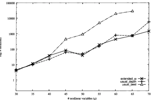
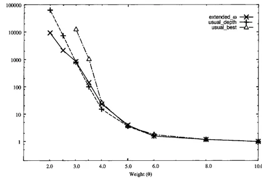
(8) 174. 5. Numerical results. In this. section,. we. report the numerical results comparing the extended. $\omega$ ‐subdivision. rule. with other subdivision rules. The test. those rules is. rating. a convex. problem solved using the simplicial algorithm incorpo‐ quadratic maximization problem of the form:. f(\mathrm{x})+ $\theta$ \mathrm{d}\mathrm{y}. maximize. subject to \mathrm{A}\mathrm{x}+\mathrm{B}\mathrm{y}\leq \mathrm{b}. (12). [x,y] \geq 0,. ,. where. f(\displayst le\mathrm{x})=\frac{1}2\mathrm{x}^{\mathrm{T}\mathrm{Q}\mathrm{x}+\mathrm{c}\mathrm{x}. To make the feasible set. bounded, the. vector. \mathrm{b}\in \mathbb{R}^{m}. was. fixed to. [ 1.0,. \cdots. ,. 1.0, n]^{\mathrm{T} and all. components of the last rows of \mathrm{A}\in \mathbb{R}^{m\times q} and \mathrm{B}\in \mathbb{R}^{m\times(n-q)} were set to 1.0. Other entries of A and \mathrm{B} together with components of \mathrm{c}\in \mathbb{R}^{q} and \mathrm{d}\in \mathbb{R}^{n-q} were generated randomly in ,. the interval. and 10%, entries. ,. [-0.5, 1.0]. respectively.. were. ,. that the percentages of The matrix \mathrm{Q}\in \mathbb{R}^{q\times q} was so. random numbers in. and. negative numbers were about 20 symmetric, tridiagonal, and the tridiagonal. zeros. [0.0, 1.0].. Note that the. part f with its. objective function of (12) can be linearized by replacing only the nonlinear concave envelope. Therefore, we may implement the branching process in the. of dimension q\leq n instead of in the whole space of dimension n Based on this decomposition principle [5], we coded the algorithm extended‐omega in GNU Octave 4.0.0 \mathrm{x} ‐space. .. ,. computing environment similar to MATLAB, tested it on one core of Intel (4.00\mathrm{G}\mathrm{H}\mathrm{z}) In order to compare the performance, we also coded the usual simplicial algorithm in two ways, one of which chooses the successor S^{i+1} of the current simplex S^{i} in [2],. a. numerical. Core i7. .. algorithm extended‐omega. usual‐depth, and the code of extended‐omega as extended tu. As the procedure for solving \overline{\mathrm{Q} (S) we used the revised simplex algorithm, which was not an optimization toolbox procedure but coded from scratch in Octave. Furthermore, we did not adopt the pruning criterion $\beta$_{S}-$\alpha$^{i}\geq $\epsilon$ in each octave best‐first order, and the other does in. depth‐first order,. We refer to the former Octave code. as. as. in the. usual‐best, the latter. as. ,. code, Uut instead used. $\beta$_{S}-(1+ $\epsilon$)$\alpha$^{i}\geq 0, where. $\epsilon$ was set to. 10^{-5}. ,. so as to. avoid the influence of the. magnitude. of the. optimal. value. the convergence. The number N prescribing the frequency of bisection in extended‐omega was fixed at 50. As varying m,n,q and $\theta$ we solved ten instances of (12) and measured the on. ,. performance of each code for each set of the parameters. Figures 1 and 2 plot the changes in the average number of iterations and the average CPU time in seconds, respectively, taken by each Octave code when the dimensionality q of \mathrm{x} increased from 30 to 70, with (m,n, $\theta$) fixed at (60, 100,5.0). Figures 3 and 4 show the results when the weight $\theta$ in the objective function changed between 2.0 and 10.0, with (m,n,q)=(60,100,30) We see from Figures 1 and 3 that extended‐omega and usual‐depth behave rather similarly and require less iterations than usual‐best. However, Figures 2 and 4 indicate that extended‐omega is rather faster than usual‐depth in terms of CPU time. The computational results for extended‐omega and usual‐depth on larger‐scale instances are sum‐ average. ..

(9) 175. \hat{underlioBms}\ne{fracitymho}. \underli{*\chek irc\math{b}0. 30. 35. 40. 45. 50. 55. \# nonlinear variables. Figure. 30. 1: Number of iterations when. 35. 40. 45. (m,n, $\theta$)=(60,100,5.0). 50. 55. \# nonlinear variables. Figure. 2: CPU time in seconds when. 60. 65. 70. 65. 70. (q). .. 60. (q). (m,n, $\theta$)=(60,100,5.0). ..

(10) 176. \hat{mring\athm{d} rs\inftya}. \underli{ot* $\hea}d{cir0mtn. 2.0. 3.0. 4.0. 6.0. 5.0. 8.0. 10.0. Weight (e). Figure. 3: Number of iterations when. (m,n,q)=(60,100,30). .. \hat{ildemrC}JD 0\Lftighaowu$me}. \chek{undrlie{\mathrQ}\mathr{o}^\mathr{n}. 2.0. 3.0. 4.0. 6.0. 5.0. 8.0. 10.0. Weight (e). Figure 4:. CPU time in seconds when. (m,n,q)=(60,100,30). ..

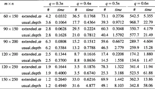
(11) 177. Table 1:. Computational results. \displaystyle \frac{q=0.3n}{\# time}\frac{q=0.4n}{\# time}\frac{q=0.5n}{\# time}\frac{q=0.6n}{\# time}. m\times n. 60\times 150. of extended‐omega when $\theta$=5.0.. \mathrm{e}x\mathfrak{t}\mathrm{e}\mathrm{n}\mathrm{d}\mathrm{e}\mathrm{d}_{-} $\omega$. 4.2. 0.0332. 36.5. 0.1768. 73.1. 0.2736. 542.5. 5.355. \displaystyle\frac{\mathrm{u}\mathrm{s}\mathrm{u}\mathrm{a}1_{-}\mathrm{d}\mathrm{e}\mathrm{p}\mathrm{t}\mathrm{h}3.60.106417. 0.436439.30.9712968.72 .79}{90\times150\mathrm{e}\mathrm{x}\mathrm{t}\mathrm{e}\mathrm{n}\mathrm{d}\mathrm{e}\mathrm{d}_{-}$\omega$2.80. 62829.50.2 2460.30.3048350.74.179} \displaystyle\frac{\mathrm{u}\mathrm{s}\mathrm{u}\mathrm{a}1_{-}\mathrm{d}\mathrm{e}\mathrm{p}\mathrm{t}\mathrm{h}2.80.162821.0 .781240.41.579257 .721.49}{90\times20 \mathrm{e}x\mathrm{t}\mathrm{e}\mathrm{n}\mathrm{d}\mathrm{e}\mathrm{d}_{-}$\omega$6.30. 80815.20.151259.60.6 72 89.74.604} \displaystyle\frac{\mathrm{u}\mathrm{s}\mathrm{u}\mathrm{a}1_{-}\mathrm{d}\mathrm{e}\mathrm{p}\mathrm{t}\mathrm{h}6.20.3 8413.20.7 8 46.52.7 9259. 15.28}{120\times20 \mathrm{e}\mathrm{x}\mathrm{t}\mathrm{e}\mathrm{n}\mathrm{d}\mathrm{e}\mathrm{d}_{-}$\omega$2.50.134 8.70.161617.40.2 08174.21.8 0} \displaystyle \frac{\mathrm{u}\mathrm{s}\mathrm{u}\mathrm{a}1_{-}\mathrm{d}\mathrm{e}\mathrm{p}\mathrm{t}\mathrm{h}2.50.370 8. 0.863614.51.\cdot5 8134.61 .47}{120\times250\mathrm{e}\times\mathrm{t}\mathrm{e}\cap \mathrm{d}\mathrm{e}\mathrm{d}_{-}\mathrm{r}o1.90.164 3.50.187678.3132 341.41 .94} \displaystyle\frac{\mathrm{u}\mathrm{s}\mathrm{u}\mathrm{a}1_{-}\mathrm{d}\mathrm{e}\mathrm{p}\mathrm{t}\mathrm{h}1.90.40 03.50.674025.3 .18 523.561.8 }{150\times250\mathrm{e}\mathrm{x}\mathrm{t}\mathrm{e}\mathrm{n}\mathrm{d}\mathrm{e}\mathrm{d}_{-}$\alpha$J1.20.26403 .0 .6216 9. 14 2362.313.86} usual‐depth. 1.2. 0.4940. 31.6. 4.877. 49.1. 8.103. 342.8. 58.06. . lists the average number of iterations and the column labeled time the average CPU time in seconds when (m,n,q) ranged up to (150,250,150), with $\theta$ fixed at 5.0. For each particular (m,n,q) again, we see that ex‐ marized in Table 1, where the column labeled. \#. ,. tended‐omega performs better than usual‐depth, especially when the proportion of nonlinear variables q/n is relatively large. These results suggest us not worry unnecessarily about the disadvantage (i) of \overline{\mathrm{Q} (S) par‐ ticularized in Section 3.. References. [1] Borovikov, V., On the intersection of a sequence of simplices (Russian), Uspekhi Matematicheskikh Nauk 7 (1952), 179‐180. [2] GNU Octave, http: / \mathrm{w}\mathrm{w}\mathrm{w}.gnu.org/software/octave/. [3] Horst, R., An algorithm for. gramming. 10. (1976),. nonconvex. programming problems. Mathematical Pro‐. 312‐321.. [4] Horst, R., P.M. Pardalos, and N.V. Thoai, Introduction Verlag (Berlin, 1995). [5] Horst, R., and H. Tuy, Global optimization: Springer‐Verlag (Berlin, 1996).. to. Global. Deterministic. 0ptimization, Springer‐ Approaches,. 3rd ed.,.

(12) 178. [6] Jaumard, B., and C. Meyer, A simplified convergence proof for the algorithm, Journal of Global 0ptimization 13 (1998), 407‐416.. cone. partitioning. [7] Jaumard, B., and C. Meyer, On the convergence of cone splitting algorithms with $\omega$subdivisions, Journal of optimization Theory andApplications 110 (2001), 119‐144. [8] Kuno, T., and P.E.K. Buckland, A convergent simplicial algorithm with $\omega$ ‐subdivision and $\omega$ ‐bisection strategies Journal of Global optimization 52 (2012), 371−390.. [9] Kuno, T., and T. Ishihama, A convergent conical algorithm with $\omega$ ‐bisection for concave minimization Journal of Global 0ptimization 61 (2015), 203‐220. [10] Kuno, T., and T. Ishihama, A generalization of $\omega$ ‐subdivision ensuring convergence of the simplicial algorithm Computational 0ptimization and Applications 64 (2016), 535‐555.. [11] Locatelli, M., Finiteness of conical algorithm with gramming A 85 (1999), 593‐616.. $\omega$ ‐subdivisions,. Mathematical Pro‐. [12] Locatelli, M., and U. Raber, On convergence of the simplicial branch‐and‐bound algo‐ rithm based on $\omega$ ‐suUdivisions, Journal of 0ptimization Theory and Applications 107 (2000), 69‐79. [13] Locatelli, M., and U. Raber, Tiniteness result for the simplicial branch‐and‐bound algo‐ rithm based on to‐subdivisions, Joumal of 0ptimization Theory and Applications 107 (2000), 81‐88. [14] Locatelli, M., and F. Schoen, Global 0ptimization: Theory, Algorithms, and Applica‐ tions, SIAM (PA, 2013). [15] Martin, R.K., Large Scale Linear And Integer 0ptimization Kluwer (Dordrecht, 1999).. —A. [16] Thoai, N.V., and H. Tuy, Convergent algorithms for minimizing Mathematics of Operations Research 5 (1980), 556‐566.. Unified Approach,. a concave. function,. [17] Tuy, H., Concave programming under linear constraints, Soviet Mathematics 5 (1964), 1437−1440.. [18] Tuy, H., Normal conical algorithm for concave minimization matical Programming 51 (1991), 229‐245.. over. polytopes. Mathe‐. [19] Tuy, H., ConvexAnalysis and Global optimization, Springer‐Verlag (Berlin, 1998)..

(13)