研
究
論 文
10 MV x - ray scatter
dose - spread
kernel
construction
using
the Bjarngard
scatter
factor
expression
Akira Iwasaki
School of Allied Medical Sciences, Hirosaki University
Research Code No.: 203
Key words: scatter factor, scatter - maximum ratio, differential scatter method , scatter dose - spread kernel, 10 MV x .rays
Abstract
The scatter factor (SF) formalism which Bjarngard has developed is so constructed that it can be applied to any high - energy photon beam, containing the in - water attenuation coefficient as a variable. However, it has not been confirmed that the SF formalism can reasonably be applied to small depths where longitudinal electron equilibrium does not exist and to small fields where lateral electron equilibrium does not exist. A method has been proposed to obtain reasonable SF data at such small depths and fields using the characteristics of a scatter dose - spread kernel . A 10 - MV x- ray scatter dose - spread kernel is given which is produced based on the SF formalism . Received Dec. 2, 1999 ; revision accepted Jan. 8, 2000
1. Introduction -
The absorbed dose at a point in a medium irradiated by photons can be separated into two components. One is the primary absorbed dose, arising from the charged secondary particles which are produced directly by primary photons. The other is the scatter absorbed dose , originating from all points hit by primary photons. When calculating the absorbed dose at a point in a medium irradiated by photons, one effective calculation method is to separate the absorbed dose into primary and scatter absorbed dose components. Cunningham l) has proposed a method of employing the zero - area tissue - air ratio (TAR) and scatter - air ratio (SAR) functions for calculation of primary and scatter absorbed dose components. The in - air absorbed dose is used for production of TAR and SAR data. For very high - energy photons, it is generally difficult to measure in - air absorbed doses at small fields accurately (there are cases where not all of the buildup cap is irradiated) . On the other hand, Khan et al.2) have proposed a method of employing the zero - area tissue - maximum ratio (TMR) and scatter - maximum ratio (SMR) functions for calculation of primary and scatter
absorbed dose components.
The convolution (or superposition) method is convenient for three - dimensional (3D) primary and
scatter absorbed dose calculations especially when using irregular fields with non - uniform incident
beam intensity. This method uses primary and scatter dose-spread kernels (or arrays) for primary
and scatter absorbed dose calculations, respectively. These kernels are usually produced3)-7) using
Monte Carlo simulations. On the other hand, Iwasaki8)-1°) has developed a method to generate
primary dose - spread kernels by analyzing the zero - area TMR in semi -infinite and finite water
phantoms. Each of these kernels is expressed by a pair of forward and backward primary
dose - spread functions. Using the differential scatter concept, 1)P11)
Iwasaki91°) has also developed a
method to generate scatter dose - spread kernels by analyzing the SMR -based scatter absorbed
dose in semi - infinite and finite water phantoms. These kernels are expressed by a pair of forward
and backward scatter dose - spread functions.
This paper uses SMR - based scatter dose - spread kernels. For a water phantom, we take points
(,r) and (Thr) on a cylindrical coordinate system whose
and 77 axes coincide with a fanline
emanating from the source (Fig. 1). Then K1 (,r) expresses the forward scatter dose components at
point (,r), arising from the origin 0 [(= 0, r= 0)] per
unit water collision kerma and per unit volume at
the origin 0, and K2 (lb
r) expresses the backward
scatter dose components at point (n,r), arising from
the origin 0 [(n= 0, r= 0)] per unit water collision
kerma and per unit volume at the origin 0.
The K1 and K2 scatter dose - spread expressions
also contain constants
of K0 and 2. Strictly
speaking, the SMR, K0, and Ti should be obtained
for the corresponding fanline; however, in this paper
we simply use SMR, K0, and IL data obtained for the
beam axis as follows. SMR(z,r) is defined as the
amount of scatter absorbed dose at a point in water
at a depth z on the beam axis for a circular field
with radius r, divided by the maximum primary
absorbed dose at the same point in water. K0 is
defined as the incident primary water collision
kerma at a point in free space on the beam axis,
divided by the maximum primary absorbed dose at
the same point in water.12)'13)
It should be noted that
all primary absorbed dose components used in this
paper are under conditions of lateral electronic
equilibrium. Au
is the average attenuation coefficient
for the primary radiation along the beam axis in a water phantom, where the attenuation coefficient is assumed to be a function of depth.
The forward scatter dose — spread function can then be expressed9)'10) as
On the other hand, the backward scatter dose — spread function for the fanline can be expressed9)3°)
In the above, a new physical quantity is employed using ?I (water phantom thickness). It is the
backscatter dose ratio (BSR). BSR(i,r) is defined as the backscatter absorbed dose at the beam —
axis incident surface point of a water phantom with thickness r for a field radius of r, divided by the
maximum primary absorbed dose at the same point within a semi —
infinite water phantom. In
previous papers,9)-11) the backscatter factor (BSF) is used instead of the BSR. The fir) function has
been introducedl° so that we can have Ki(0,r)=K2(0,r).
The scatter factor (SF) is defined") as the ratio of total absorbed dose to primary absorbed dose at
a point in water at a depth on the beam axis. TMR(z,O) expresses the zero —
area TMR for a depth z
in water on the beam axis. The zero —
area TMR is defined as the primary absorbed dose at a point
in water on the beam axis, divided by the maximum primary absorbed dose at the same point in
water. Using the above —
defined SMR and zero —
area TMR functions, the SF at depth z for a field
radius r can be given by
We let the primary radiation attenuation coefficient along the beam axis be expressed as fi.(z) and we put ,u0=y(0) (see the Appendix). Bjarngard and colleagues1516) have found that the SF can be approximated by
with ao=yo and wo = 1.73— 17.1,uo, where z and r are expressed in cm, ao and ,u0 are in cm-1, and wo is dimensionless.
Equation (6) has been constructed in the region which is under conditions of lateral and longitudinal electron equilibria. Equation (6) leads to SF(z,r) =1 for z = 0 for any given value of r. This means that the backscatter dose calculated on the incident surface is zero for any field size. Therefore, it can be understood that Eq.(6) is unreasonable at least at depths near z=0. On the other hand, it is reasonable that Eq.(6) leads to SF(z,r)=1 for r= 0; however, it is not guaranteed that Eq. (6) is valid for small field sizes.
This paper describes a method of deriving 10 MV x—ray SF (or SMR) data at small depths and fields from the original SF formalism of Eq.(6), and then produces a 10 MV x — ray scatter
dose — spread kernel using the K1 and K2 functions.
2. Methods
A. For small depths
We modify the right side of Eq.(6) by replacing z by_ a function g(z) so that we can have SF(z,r) 1 for z=0. We let zo be a certain value of z below which Eq.(6) can not hold reasonably. For z zo we rewrite Eq.(6) as
where Ii and 12 are constants. We simply determine the values of the constants as f2 = 1/4 and Ii =zo
exp(—fazo) using the relations Azo)=zo and e(z0)= 1 [Eqs.(6) and (7) can be connected smoothly at
z=z0j. Then we can have SF(0,r) < 1 for any non—zero value of r. Therefore, Eq.(5) leads to
B. For small fields
It can be seen that Eqs.(9) and (10) can not produce a finite K gr) value at r= 0 for any value of We re — evaluate the SMR for small values of r as follows. We let ro be a certain value of r below which Eqs.(9) and (10) can not hold reasonably. According to Iwasaki,17"8) the SMR for small field
radii of r < 7'0 should be expressed as
Jpn. J. Med. Phys. Vol.19. No.4 V4-1-NIX:14-*"' 19 4 14
where the values for F1(z) and F2(z) are obtained by setting SMR(z,r) and aSMR(z,r)/ ar of Eq.(11) equal to SMR(z,r) and aSMR(z,r)/ ar of Eq.(9) or (10), respectively, for r= ro.
3. Experiments and results
The experimental study was made on a Mitsubishi ML —15 M linear accelerator, producing 10 MV x rays. All experiments and calculations were performed along the beam axis. As the primary radiation attenuation coefficient expression in water on the beam axis, we employed13)'19)
where z is in cm and p(z) in cm-1 (see the Appendix). As the average attenuation coefficient (ü), we
employed 12=0.0365 cm-1 (see the Appendix). The value for zo used in Eq.(6) was yo=0.0391 cm-1
[=2(0)]. Therefore, we obtained ao = 0.0391 cm-1 and wo=1.061, which were used in Eqs.(6), (7), (9),
and (10). The value for Ko used in Eqs.(1) and (2) was Ko=1.11678.13)
As the zero —
area TMR expression on the beam axis, we used13)
where To=1.14838, Co= —100, U0=100.02935, a =1.28013 cm-1, and b =1.27999 cm-1. The depth
of maximum primary absorbed dose was zmax=2.779 cm [dTMR(z,0)/dz
=0 for z=zmax].
A. The values for ro and zo
We introduced another expression K1(t,0). It is reconstructed by setting =.'t cos° and r=t sin0 for IC1(',r) (see the inset in Fig. 3 below), where t is the distance of point (",r) from the origin along the fanline with an inclination of 0 against the axis.
In order to determine the values of ro and zo, we place the following three restrictions.
(a) Restriction 1: The SMR(z,r)/TMR(z,0) curve for any non—zero r value should increase with increasing z (refer to Fig. 6 below).
(b) Restriction 2: The K1(t,0) curve should decrease with increasing t (refer to Fig. 3 below). (c) Restriction 3: The relation K1(t,01) > Ki(t,02) for 01 < 02 should be obtained for any non—zero value of t (because high — energy radiation like 10 MV x rays is scattered forward strongly).
It has been found that restriction 1 can be satisfied for any values of ro and zo. Figure 2 shows the regions of 7.0 and zo values satisfying restrictions 2 and 3. The common region satisfying restrictions
2 and 3 is almost on a line from the point of ro = 0.615 cm and zo=1.055 cm to the point of 7-0=1.091 cm and 2'0=1.198 cm. We employed r0=0.615 cm and zo =1.055 cm. This is because K1(,r) with these ro and zo values can make a scatter dose — spread kernel which is more like Monte Carlo generated ones3)-7) near the origin 0 (=.0 and r= 0).
negative values of the order of —10-32 to —0 in a limited region of i and r, where a2BSR(72,r)/ an ar is expressed as
then we can obtain K2(i1,r) 0 for all values of i and r, keeping K1(0,r)=K2(0,r). In the following, we used Eq.(15) for calculation of K2(,,r).
B. Distributions of K1(,r) and K2(r1,r) values
Using Eqs.(9)—(11) with (4)=0.0391 cm-1, w0=1.061, ro = 0.615 cm, and zo =1.055 cm and using Eq.(13), we derived K1(,r) and K2(7),r) values. It can be understood from the K1(,r) and If2(Thr) definitions that their units are cm-3 when using a system of cm units for , n, and r.
Jpn. J. Med. Phys. Vol.19. No.4
seen from Fig. 3, the curves exhibit relatively large slope changes at points satisfying t= 0. 615/sine (cm) and t=1.055/cos0 (cm). From the insert in Fig. 4, we introduce a function K2(t,0) similarly. Figure 4 shows a set of K2(t,0) curves along fanlines emanating from the origin 0 (77=0, r= 0). The curve with 0=90° shows a relatively large slope change at the point t= 0.615 cm.
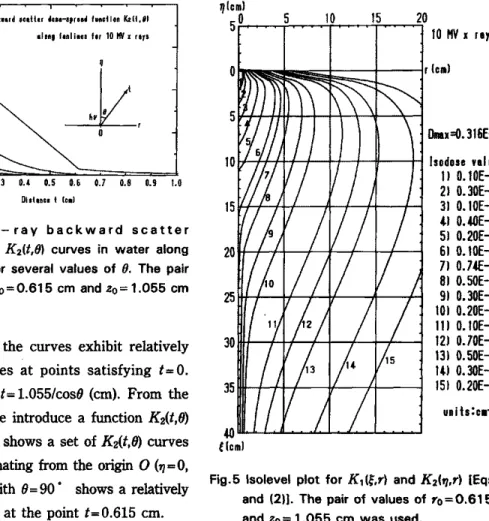
Figure 5 shows a set of K1(,r) and K2(ij,r)
isodose lines in water, constructed using Eqs.(1) and (2). Both K1(,r) and K2(n,r) functions take the same maximum value of 0.0316 cm-3 at the origin. When compared with Monte Carlo generated kernels,3)-7) the following characteristics are obtained: the K2(,,r) contribution is relatively small (the reason is described in section 4); the K1(,r) isodose lines show slightly unnatural patterns in the region < 1.055 cm (=z0); and the KI(I'M isodose lines with 0.74E-04 cm and less exhibit a tail — like isodose pattern around the axis when the value of is large.
According to Ahnesj6,7) the scatter dose — spread kernel should have an infinite value at the primary photon interaction point; namely, K1(0,0) =oo and K2(0,0) =oo . However, this stipulation can not be applied to the K1 and K2 functions.
C. SMR(z,^)/TMR(z,O) values
In this subsection, as the variable of field size we take the square field side (s) instead of the circular field radius (r). According to Bjdrngard and Siddon,") the equivalent square and circular fields have the following relationship:
For the present 10 MV x— ray radiation, the minimum square field size providing full lateral electronic equilibrium at deep points in water on the beam axis is 3.5 X 3.5 CM2.17) Two kinds of SMR fitting expressions have been reported1m18)
as a function of square field side (s) and depth (z). This paper employs another kind of SMR fitting expression, which has been constructed using SMR data obtained for z= 4-30 cm and s= 5-30 cm with the zero — area TMR of Eq.(13). It is given by
where z and s are in cm. The values for G1(z) and G2(z) are determined by setting SMR(z,^) and aSMR(z,^)I a s of Eq.(17) equal to SMR(z,^) and i;SMR(z,^)I as of Eq.(21), respectively, for s = 3.5 cm. As may be seen from the results shown in Fig. 6 below, Eq.(17) is valid at depths of about 1-30 cm. Figure 6 shows three sets of SMR(z,^)/TMR(z,0) values for depths of z 40 cm and square field sides of s 30 cm, where Eq.(13) was used for TMR(z,0). The first was produced using SMR data which were acquired using Eqs.(9)—(11) and (16), shown by the solid lines; the second was produced using SMR data which were acquired using Eqs.(17) and (21), shown by the broken lines; and the third was produced using a set of measured SMRs, shown by the dotted lines. From Fig. 6, we see the following points.
(a) In the region of — 5 cm <z <— 30 cm, the three sets coincide well with each other. (b) The broken lines show unreasonable values at depths of z > — 30 cm. This effect becomes more pronounced as the field size increases.
(c) The broken lines show unreasonable values near the depth of z =0 cm.
It can be understood that the solid lines express the most reasonable SMR(z,^)/TMR(z,0) data. Therefore, we may state that the SMR(z,^)/TMR(z,0) function should be a continuously increasing function with depth z for any non — zero s value (restriction 1).
D. Another type of scatter dose — spread kernel
We produced another kind of scatter dose — spread kernel, where we used the same parameters as when we produced the kernel of Fig. 5; however, we let the value of 7-0 be a function of , as given by
where ro and
are expressed in cm. Figure 7 illustrates the result. This kernel does not exhibit
tail —
like isodose lines like Fig. 5 does. It is more like Monte Carlo generated kernels.3)-7)
Figure 8 shows a set of SMR(z,^)/TMR(z,0) curves, where TMR(z,0) was evaluated using Eq.(13)
and SMR(z,^) was evaluated using Eqs.(9) —
(11) and (16) with s0(z)
= ro(z)/0.561 [refer to Eq.(22)]. The
SMR(z,^)/TMR(z,0) curves at small fields are not continuously increasing functions with depth z (not
satisfying restriction 1); namely, they are not reasonable. Therefore, it can be understood that such
tail —
like isodose patterns as shown in Fig. 5 certainly have an important role when using the
Bjarngard scatter factor (SF) formalism.
4. Discussion
For 1.25-18 MeV incident photon energies, McGary et al.21) have compared first scattered point
dose arrays generated by a Monte Carlo method and an analytic method, where the analytic method
models energy deposition using Klein—Nishina
cross sections for Compton scatter
and
approximations for electron transport. They concluded that there was good agreement for the
forward scatter volume, but significant differences appeared within the backscatter regions where
the analytical method made approximations. Therefore, the tail—like isodose patterns shown in Fig.
5 must be unreasonable.
For the present 10 MV x —
ray radiation, Iwasaki17) has reported that the minimum square field
side with complete lateral electronic equilibrium in water on the beam axis is s 3.5 cm with respect
to the primary plus scatter absorbed dose component (almost the same value may also be adapted to
the case of the pure primary absorbed dose component) and that the minimum depth with complete
longitudinal electronic equilibrium in water on the beam axis is z = 6 cm with respect to the primary
absorbed dose component. These s and z values are much larger than the values of so
=1.096 cm and
zo =1.055 cm, respectively, obtained for the Bjarngard SF formalism. This fact suggests that the
Bjarngard SF formalism can be valid even at points where the lateral and longitudinal electronic
equilibria are partly broken.
The original Ka")
and K2(Thr) functions have been derived in a paper by Iwasaki and Ishito.11)
From this paper and another,9) the following three facts can be obtained.
(a) The scatter absorbed dose calculated by convolution using Eqs.(1) and (2) for a point at a depth
Z on the beam axis with a circular field of radius R becomes exactly SMR(Z,R) if the beam is
parallel, if the irradiated medium is a semi—infinite water phantom, if the beam attenuation
coefficient along raylines is not a function of depth and off —
axis distance, and if the incident beam
intensity is Ku within the field and zero outside the field.
(b) Strictly speaking [refer to Fig. 9(0], the Ki(,r) function expresses the amount of forward scatter absorbed dose for point (,r) in a semi — infinite water phantom per unit primary water collision kerma per unit volume at the interaction point (= 0, r= 0) situated on the pencil—beam entry surface.
(c) Strictly speaking [refer to Fig. 9(b)], the If2(Thr) function expresses the backward scatter absorbed dose for point (i,r) on the pencil—beam incident surface of a water phantom with thickness ri per unit primary water collision kerma per unit volume at the interaction point (77 = 0, r=0) situated on the pencil — beam exit surface. Therefore, we can understand one reason why the KAT/A function produces a smaller scale dose distribution as shown in Fig. 5. Another reason may be caused by the mathematical restriction of Ki(0,r)=K2(0,r) used for deriving the f(r) function of Eq.(4).
On the other hand, the primary and scatter dose—spread kernels which have been produced by the Monte Carlo approach usually have their interaction point forced to the center of a large water phantom. When using such kernels for convolution methods, a worst—case error is introduced22) near the beam incident surface since the primary and scatter dose perturbation beyond the boundary of the phantom is not taken into account. However, AhnesjO22) has pointed out that such an error can be neglected with respect to both primary and scatter absorbed dose components.
5. Conclusions
On the basis of the Bjdrngard scatter factor (SF) formalism, we have proposed a method for obtaining reasonable SF data at small depths and fields where longitudinal and/or lateral electronic equilibria do not exist. A 10 MV x—ray scatter dose — spread kernel was constructed using a pair of forward and backward scatter dose — spread functions in which the scatter — maximum ratio (SMR) was evaluated using the SMR — SF relationship.
Acknowledgments
This work was done using 10 MV x — ray data measured by personnel of Aomori Kousei Hospital . The author would like to express his appreciation to Dr. T. Ishikawa.
Appendix: The 10 MV x — ray attenuation expression
The method for constructing the 10 MV x —ray primary radiation attenuation coefficient expression used in this paper is detailed in Ref.19. We take a point in water with a depth of z (cm) on the beam axis. Then the attenuation coefficient (cm-1) for the point can be approximated as
attenuation coefficient of water among the spectrum lines whose energy fluences are not zero.
Equation (Al) is so constructed that we can have 12(00)=yinin
(= the attenuation coefficient for 10
MeV photons).
The average (or effective) attenuation coefficient (ji=0.0365 cm 1) is obtained from the slope of a
straight line that is drawn under the assumption that the exp[mu(z)z] data at z= 0-30 cm decrease
linearly with increasing depth (z) on semilog graph paper. In this case we have IL k- y(30).
Bjàrngard and Shackford23) have proposed the following attenuation coefficient expression:
/t(z)
=tici(l
noz)
(A2)
where A0[=y(0)] and no are constants. The values for yo and no can be derived by setting exp(—goz)
=1 —goz
in Eq.(A1), as
/20 =f0 //min (A3)
=fo - go/yo. (A4)
References
1) Cunningham JR: Scatter—air ratios. Phys Med Biol 17:42-51, 1972
2) Khan FM, Sewchand W, Lee J, and Williamson JF: Revision of tissue—maximum ratio and scatter — maximum ratio concepts for cobalt 60 and higher x—ray beams. Med Phys 7: 230-237,
1980
3) Mackie TR, Scrimger JW, and Battista JJ: A convolution method of calculating dose for 15—MV x rays. Med Phys 12: 188-196, 1985
4) Mohan R, Chui C, and Lidofsky L: Differential pencil beam dose computation model for photons. Med Phys 13: 64-73, 1986
5) AhnesjO A, Andreo P, and Brahme A: Calculation and application of point spread functions for treatment planning with high energy photon beams. Acta Oncologica 26: 49-56, 1987 6) Mackie TR, Bielajew AF, Rogers DWO, and Battista JJ: Generation of photon energy deposition
kernels using the EGS Monte Carlo code. Phys Med Biol 33: 1-20, 1988
7) AhnesjO A: Collapsed cone convolution of radiant energy for photon dose calculation in heterogeneous media. Med Phys 16: 577 —592, 1989
8) Iwasaki A: Calculation of three — dimensional photon primary absorbed dose using forward and backward spread dose—distribution functions. Med Phys 17: 195-202, 1990
9) Iwasaki A: 10 — MV x — ray primary and scatter dose calculation using convolutions. Med Phys 17: 203-211, 1990
10) Iwasaki A: A convolution method for calculating 10— MV x — ray primary and scatter dose including electron contamination dose. Med Phys 19: 907-915, 1992
11) Iwasaki A and Ishito T: The differential scatter - air ratio and differential backscatter factor method combined with the density scaling theorem. Med Phys 11: 755 - 763, 1984
12) Iwasaki A: A method of calculating high - energy photon primary absorbed dose in water using forward and backward spread dose - distribution functions. Med Phys 12: 731- 737, 1985 13) Iwasaki A: A 10 MV x -ray zero - area tissue - maximum ratio expression constructed by taking
into account depth and off axis beam quality change. Med Phys 25: 2209 -2214, 1998 14) Day MJ and Pitchford WG: The normalized peak scatter factor and normalized scatter functions
for high energy photon beams. In Central Axis Depth Dose Data for Use in Radiotherapy: 1996. Brit J Radiol Supplement 25: 168 -176, 1996
15) Bjarngard BE, Vadash P, and Ceberg CP: Quality control of measured x - ray beam data. Med Phys 24: 1441-1444, 1997
16) Bjarngard BE and Vadash P: Relations between scatter factor, quality index and attenuation for x -ray beams. Phys Med Biol 43: 1325-1330, 1998
17) Iwasaki A: 10 MV x ray SMRs obtained using zero area Sp correction factors derived by means of the Bjarngard - Petti method. Phys Med Biol 41: 625 - 636, 1996
18) Iwasaki A: 10 MV x- ray zero - area phantom scatter correction factors (Sr) obtained using three extrapolation methods. Phys Med Biol 41: 2627 -2634, 1996
19) Iwasaki A: A 10 MV x - ray attenuation coefficient expression for water as a function of depth and off - axis distance. J Jpn Soc Ther Radiol Oncol 10: 53-60 1998
20) Bjarngard BE and Siddon RL: A note on equivalent circles, squares, and rectangles. Med Phys 9: 258-260, 1982
21) McGary JE, Boyer AL, and Mackie TR: A comparison of Monte Carlo and analytic first scatter dose spread arrays. Med Phys 26: 751 -759, 1999
22) AhnesjO A: Invariance of convolution kernels applied to dose calculations for photon beams. Proc 9th Int Conf on the Use of Computers in Radiation Therapy: 99 102, 1987
23) Bjarngard BE and Shackford H: Attenuation in high energy x - ray beams. Med Phys 21: 1069-1073, 1994