21
Nonexistence ofbifurcation from Crapper’s pure capillary waves*
HISASHI OKAMOTO AND MAYUMI SHOJI
岡本 久 東海林 まゆみ
\S 1.
Introduction.We consider a free boundary problem of progressive waves of two dimensional
ir-rotational flow of inviscid incompressible fluid. In [1] Crapper showed that this free
boundary problem has a family of solutions expressed by elementary functions in the
case where the gravity is neglected and only the capillary force is taken into account.
The purpose of the present paper is to prove that there is no bifurcation from this
family of solutions, in other words, this family is isolated from any other solutions.
The reason that we give a complete but rather elementary proof is that the result
contributes to clarifying the global bifurcation diagram of the solutions. In fact, when
we take account of both the gravity and the capillary force, nulnerical simulations
show that there is a rather complicated bifurcation structure including secondary
bi-furcations in the set of the solutions ([6,7]). Yet, in the limit of zero gravity, our
theorem implies that no secondary bifurcation is possible.
The present paper consists of five sections. The precise mathematical formulation is givenin
\S 2.
Basic facts onCrapper’s waves are briefly reviewed in\S 3.
Theorem andits proofis given in
\S 4.
We present some numerical results in \S 5, which visually showthe meaning of our theorem and seems, at the same time, to indicate the following
conjecture: only Crapper’s waves are solutions when the gravity is zero.
\S 2.
Formulation ofthe problem.We take a coordinate system $(x, y)$ moving with the wave with thesame speed. The
x-coordinate is taken horizontally to the right and y-coordinate is taken vertically
upward. By definition, the wave profile of aprogressive wave is at rest in this moving
frame and there is an underlying flow travellingin the opposite direction. We consider
two dimensional irrotational flow of incompressible inviscid fluid. As usual in this
problem, we assume that the wave profile is periodic in $x$ with a period $L$, and is
symmetric with respect to a vertical line passing through a crest. We take theline as
y-axis. We consider a flow of infinite depth with a smooth free boundary expressed
by $y=h(x)$. Consequently it is sufficient to consider the flow in $\Omega_{h}\equiv\{z=x+iy\in$
$C;-L/2<x<L/2,$
$-\infty<y<h(x)$}.
The problem is to find an even function $y=h(x)$ $(|x|<L/2)$, and an analytic
function $f(z)$ $(z\in\Omega_{h})$ called a complex potential satisfying the following (2.1-4):
(2.1) $V=0$ on $y=h(x)$
.
(2.2) $U=\pm cL/2$ on $x=\pm L/2$, respectively.
’This work was partially supported by Ohbayashi Corporation
数理解析研究所講究録 第 745 巻 1991 年 21-38
22
(2.3) $\frac{1}{2}|\frac{df}{dz}|^{2}+gy-\frac{T}{m}(\frac{h_{x}}{\sqrt{1+h_{x}^{2}}})_{x}=constant$ on $y=h(x)$,
(2.4) $\frac{df}{dz}arrow c$ as
$yarrow-\infty$
.
where the subscript implies the differentiation, $g,$ $m$ and$T$are positiveconstantscalled
the gravityconstant, the mass density, and the surface tension coefficient, respectively.
We require that $f(z)$ is analytic in $\Omega_{h}$ and continuously differentiable (in the real
variables) in $\overline{\Omega_{h}}$. The complex potential$f(z)$ determines the velocity vector $(u, v)$ by
$u– iv=df/dz$. For the derivation of (2.1-4), see [2] or [4].
We can give an alternative formulation to this free boundary problem. The original
problem (2.1-4) is formulated by the relation between $f$ and $z$. The new formulation is
written in terms of $\zeta\equiv\exp(-2\pi if/(cL))$ and $\omega\equiv i\log(c^{-1}df/dz)$. This formulation
is due to Levi-Civita and expressed as follows. Find a
function
$\omega=\omega(\zeta)$ which iscontinuous on $|\zeta|\leq 1$, is analytic in $|\zeta|<1$ and
satisfies
$\omega(0)=0$ and(2.5) $e^{2\tau} \frac{\partial\tau}{\partial\sigma}-pe^{-\tau}\sin\theta+q\frac{\partial}{\partial\sigma}(e^{\tau}\frac{\partial\theta}{\partial\sigma})=0$ on $\rho=1$,
where $(\rho, \sigma)$ is the polar coordinate
of
$\zeta,$ $\theta=\theta(\rho, \sigma)$ is the real partof
$\omega$, and $\tau=$$\tau(\rho, \sigma)$ the imaginary part. $p$ and $q$ are nondimensional parameters
defined
by $p=$$gL/(2\pi c^{2}),$$q=2\pi T/(mc^{2}L)$. The derivation of (2.5) is given in [5]. We remark that
$\theta$ is related with the free boundary by the following relation:
(2.6) $\tan\theta=\frac{d}{dx}h(x)$.
Since an analytic function is uniquely determined by its boundary value, a
fur-ther reduction of the equation (2.5) is possible. In fact we can write (2.5) only by
$\theta(1, \sigma)$ $(0\leq\sigma<2\pi)$
.
To this end, we define aHilbert transform on $S^{1}$:$H( \sum_{n=1}^{\infty}(a_{n}\sin n\sigma+b_{n}\cos n\sigma))=\sum_{n=1}^{\infty}(-a_{n}\cos n\sigma+b_{n}\sin n\sigma)$
.
Thisis alinearisomorphismfrom$L^{2}(S^{1})/R$ ontoitself. $H(\theta(1, \sigma))$ is well-defined, since
$\int_{0}^{2\pi}\theta(1, \sigma)d\sigma=0$ is assured by $\omega(0)=0$ (see [5]). Then we have $\tau(1, \sigma)=H(\theta^{*})$,
where $\theta^{*}(\sigma)=\theta(1, \sigma)$. The equation (2.5) is now written as
(2.7) $e^{2H\theta^{*}} \frac{dH\theta^{*}}{d\sigma}-pe^{-H\theta^{*}}\sin\theta^{*}+q\frac{d}{d\sigma}(e^{H\theta^{*}}\frac{d\theta^{*}}{d\sigma})=0$ $(0\leq\sigma<2\pi)$.
Accordingly the problem is to find a $2\pi$-periodic function $\theta^{*}$ satisfying (2.7).
Equiva-lence of (2.7) and (2.5) with $\omega(0)=0$ is also shown in [5]. Obviously, $\theta^{*}\equiv 0$ satisfies
(2.7) for all $p$ and $q$
.
This is a trivial solution. In fact, (2.6) implies $h\equiv$ constant.Thus free boundary is completely flat. By the definition of $\omega,$ $\theta(1, \sigma)\equiv 0$ implies
$df/dz\equiv c$, which shows that the velocity field is uniform: $(u, v)\equiv(c, 0)$
.
Theprob-lem ofperiodic progressive water waves is to find$\theta^{*}$ which is not identically zero and
23
\S 3.
Crapper’s waves.In what follows we consider (2.5) or (2.7) in the case of$p=0$. Namely we neglect
thegravityforce and only the capillary forceis assumed. In this extremecase, Crapper
[1] found a family of solutions which are expressed by elementary functions. We put
$F(q, u)= \frac{d}{d\sigma}(\frac{1}{2}e^{2Hu}+qe^{Hu}\frac{du}{d\sigma})$ .
Thus we wish to find zeros of F. $F$ is defined in a certain Banach space, which will
be defined in the next section. Since we consider only Crapper’s special solutions in
this secton, the functional analytic formalism in the next section is not necessary here.
Note that $(q, u)$ is a zero of $F$, if $qdu/d\sigma=-\sinh(Hu)$.
THEOREM 3.1 (CRAPPER [1]). Define an analytic function $\omega$ by
(3.1) $\omega=\theta+i\tau=2i\log\frac{1+A\zeta}{1-A\zeta}$,
where $A$ is a real parameter$sati$
)
$sfying-1<A<1$
an$d$ theprincipal bran$ch$ of $log$ is$t$aken. We also define
(3.2) $q= \frac{1+A^{2}}{1-A^{2}}$
Then $u=\theta(1, \sigma)$ satisfies $F(q, u)=0$ for-l $<A<1$ .
PROOF: For $A\in(-1,1)$, the relation (3.1) defines an analytic function in the unit
disk. We have
(3.3) $\tau(1, \sigma)=2\log|\frac{1+Ae^{i\sigma}}{1-Ae^{i\sigma}}|=\log\frac{1+A^{2}+2A\cos\sigma}{1+A^{2}-2A\cos\sigma}$
$=4(A \cos\sigma+\frac{A^{3}}{3}\cos 3\sigma+\frac{A^{5}}{5}\cos 5\sigma+\cdots)$
and (3.4)
$\theta(1, \sigma)=-2$arctan $( \frac{2A\sin\sigma}{1-A^{2}})=-4(A\sin\sigma+\frac{A^{3}}{3}\sin 3\sigma+\frac{A^{5}}{5}\sin 5\sigma+\cdots)$.
It also holds that $\tau(1, \sigma)=H(\theta(1, \sigma))$ and
(3.5) $e^{\tau(1,\sigma)}= \frac{1+A^{2}+2A\cos\sigma}{1+A^{2}-2A\cos\sigma}=\frac{1+3A^{2}}{1-A^{2}}+\frac{4(1+A^{2})}{1-A^{2}}\sum_{n=1}^{\infty}A^{n}\cos n\sigma$,
and
24
These two equations give
$\sinh\tau=\frac{4(1+A^{2})}{1-A^{2}}$
(A
$\cos\sigma+A^{3}\cos 3\sigma+\cdots$).
This equality and (3.4) prove that
$q \frac{d}{d\sigma}\theta(1, \sigma)=-\sinh\tau$
.
It is now easy to check $F(q, u)=0.1$
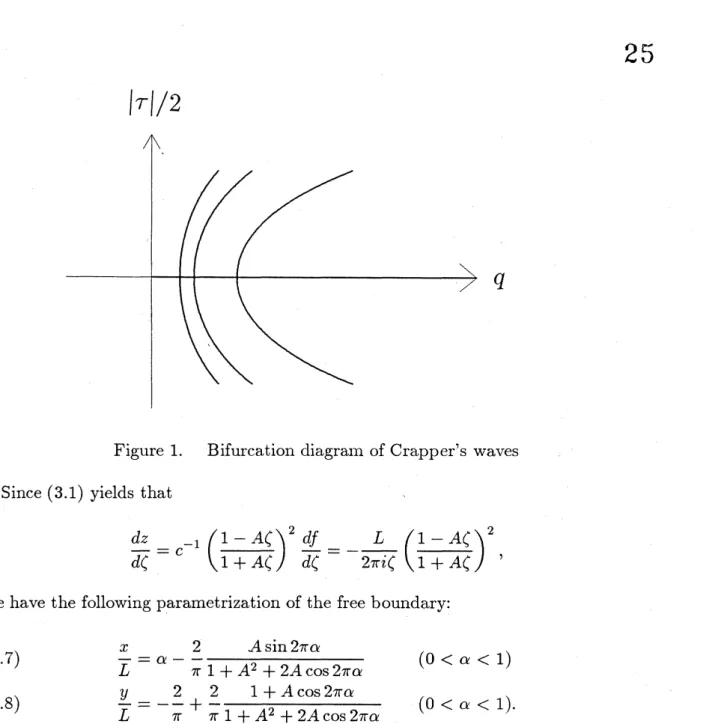
We call the solution in Theorem 3.1 Crapper’s wave. By the definition, Crapper’s wave satisfies $\omega\equiv 0$ at $q=1$
.
This means that $df/dz\equiv c$. Thus, at $q=1$,Crap-per’s wave becomes a trivial solution. In other words, CrapCrap-per’s wave bifurcates at $q=1$ from the trivial solution. (3.2) also shows that the bifurcation takes place
supercritically in $q$
.
The bifurcation diagram is illustrated by$q= \cosh(\frac{1}{2}\tau(1,0))$ ,
which follows from (3.2, 3). This curve and the trivial solutions $\{(q, 0);0<q<\infty\}$
form a pitchfork.
If we linearize $F$ at $u=0$, then we obtain the following Fr\’echet derivative:
$D_{u}F(q,0)w= \frac{d}{d\sigma}(Hw+q\frac{dw}{d\sigma})$
.
This formula yields $D_{u}F$($q$, O)(cos$n\sigma$) $=n(1-nq)\cos n\sigma$ and $D_{u}F$($q$,O)(sin$n\sigma$) $=$
$n(1-nq)\sin n\sigma$ for $n=1,2,$ $\cdots$
.
Therefore, the Frechet derivative at the trivialsolution has nontrivial kernel if and only if $q=1/n$ for some $n=1,2,$ $\cdots$
.
Thesolutions (3.4) corresponds to the one emanating from $(q, u)=(1,0)$. The solutions
bifurcating from $(q, u)=(1/N, 0)$ $(N=1,2, \cdots)$ are given by
$q= \frac{1}{N}\frac{1+A^{2}}{1-A^{2}}$ $u(\sigma)=\theta(1, N\sigma)$,
where $\theta$ is defined by (3.4). We call this family of solutions Crapper’s solutions of
25
$|\tau|/2$
$q$
Figure 1. Bifurcation diagram of Crapper’s waves
Since (3.1) yields that
$\frac{dz}{d\zeta}=c^{-1}(\frac{1-A\zeta}{1+A\zeta})^{2}\frac{df}{d\zeta}=-\frac{L}{2\pi i\zeta}(\frac{1-A\zeta}{1+A\zeta})^{2}$ ,
we have the following parametrization of the free boundary:
(3.7) $\frac{x}{L}=\alpha-\frac{2}{\pi}\frac{A\sin 2\pi\alpha}{1+A^{2}+2A\cos 2\pi\alpha}$ $(0<\alpha<1)$
(3.8) $\frac{y}{L}=-\frac{2}{\pi}+\frac{2}{\pi}\frac{1+A\cos 2\pi\alpha}{1+A^{2}+2A\cos 2\pi\alpha}$ $(0<\alpha<1)$.
By this formula we can draw the figures of the free boundaries. In Figure 2, free
boundaries with negative$A$ aregiven. Curves with positive $A$ are obtained by shifting
thosefigures $with-A$ by half a wave length. While $|A|$ is small, the wave profiles look
sinusoidal. They, however, form particular shapes for large $|A|$ and, eventually, $y$ is
not a single valued function of $x$ when $|A|>0.414215\cdots$ . If $|A|>0.454670\cdots$ , then
the free boundary has a self-intersection and becomes physically meaningless. In this
sense we redraw Figure 1 as Figure 1’, where solid curves represent physical solutions
26
A $=$ $-$ $0.414215$ A $=$ $-$ $0.1$ 0.454670 A $=$ $-$ $0.2$ 0. 5 A$=-0.3$
Figure 2
$|\mathcal{T}|/2$ $q$Figure
$1^{)}$27
Note, however, that (3.1) is well-defined for all $A\in(-1,1)$ and is a mathematical
solution to$F=0$. Computations in [7] pointedout that: acquisition of not only
phys-ical solutions with no self-intersection but also self-intersecting, unphysical solutions
is necessary for the complete understanding of global structure of the solutions. In fact, consider a bifurcation point at which the wave profile is self-intersecting. The
new bifurcating solutions near the bifurcation point are self-intersecting. The branch,
however, may go back to the region of physical solutions and there may be physically
meaningful solutions other than Crapper’s waves. A possible example is illustrated
by Figure 3, where solid curves represents physical solutions and the broken curves
do unphysical ones. Sqppose we are tracing solutions along the curve AB and find
that the solutions begin forming self-intersections. If we neglect solutions after $B$
then we clearly overlook the physical solutions C. Bifurcation of this nature do occur
when both surface tension and gravity are taken into account ([7]). This point is
explained in more detail later in
\S 4.
Accordingly we consider (3.4) for all $A\in(-1,1)$.Figure 3. Possible recovery from self-intersection
\S 4.
No bifurcation from Crapper’s waves.In this section, we prove nonexistence of a bifurcation from the branch of Crapper’s waves. In order to state a theorem precisely, we define the following function spaces
for a nonnegative integer $m$:
$X^{m}=$ $H^{m}(S^{1})/R$
$= \{f=\sum_{n=1}^{\infty}(a_{n}\sin n\sigma+b_{n}\cos n\sigma)$; $\sum_{n=1}^{\infty}n^{2m}(|a_{n}|^{2}+|b_{n}|^{2})<\infty\}$ ,
where$H^{m}(S^{1})$ is the Sobolevspace. The mapping$F$is a smooth mappingfrom $R\cross X^{2}$
28
Then $F$ sends every element of $Y^{2}$ into $Y^{0}$ ([5]). For the sake of convenience, we
write for a positive integer $N$,
(4.1) QN$(A)= \frac{1+A^{2}}{N(1-A^{2})}$ $\Theta_{N}(A, \sigma)=-2$ arctan $( \frac{2A\sin(N\sigma)}{1-A^{2}})$ .
We then have $F(Q_{N}(A), \Theta_{N}(A, \cdot))=0$ for all-l
$<A<1$
.
We note that Crapper’ssolutions (4.1) lie in $Y^{2}$.
THEOREM 4.1. For an$yN=1,2,$ $\cdots$ and any $A\in(-1,1)$ with $A\neq 0$, Crapper’s
solutions (4.1) are isolated. Namely, there is no bifurcation from Crapper’s waves
except for $(q, u)=(1/N, 0)$.
PROOF: We must be careful about the meaning of isolatedness. In fact, if $\theta(\sigma)$ is
a solution, then $\theta(\sigma+\beta)$ is a solution, too, where $\beta$ is a constant in $[0,2\pi$). In
$R\cross Y^{2}$, Crapper’s waves form a pitchfork givenby (2.2, 4). In $R\cross X^{2}$, we have a set
of solutions which is obtained by revolving the pitchfork around the q-axis. Thus we
have a bifurcationdiagram consisting of a parabolic surface and a lineintersectingwith
it. What we have to show is that any point of the parabola except for $(q, u)=(1,0)$
has a neighborhood in $R\cross X^{2}$ such that the zeros of $F$ in the neighborhood are only
those points- on the parabola.
We first calculate the Fr\’echet derivative:
(4.2) $F_{u}(q, u)w= \frac{d}{d\sigma}[e^{2Hu}Hw+qe^{Hu}\frac{du}{d\sigma}Hw+qe^{Hu}\frac{dw}{d\sigma}]$ $(w\in X^{2})$.
In what follows, we fix a positive integer $N$. We write $F_{u}(Q_{N}(A), \Theta_{N}(A, \cdot))$ as $L_{A}$.
We note that
(4.3) $F(Q_{N}(A), \Theta_{N}(A, \cdot+\beta))=0$
for all $A\in(-1,1)$ and $\beta\in[0,2\pi$). By differentiating with respect to $\beta$ and putting
$\beta=0$, we obtain $L_{A}(\partial\Theta_{N}/\partial\sigma)=0$. Differentiating (4.3) in $A$ and putting $\beta=0$, we
have
$L_{A}( \frac{\partial\Theta_{N}}{\partial A})+F_{q}(Q_{N}, \Theta_{N})\frac{\partial Q_{N}}{\partial A}=0$
.
We consider the following equation in $R\cross X^{2}$:
(4.4) $L_{A}w+\Phi_{A}\lambda=0$,
where $\Phi_{A}=F_{q}(Q_{N}, \Theta_{N})\frac{\partial Q_{N}}{\partial A}$. By the above consideration, we already have two
independent solutions to this equation, i.e.,
(4.5)
$( \lambda, w)=(0, \frac{\partial\Theta_{N}}{\partial\sigma})=(0, -4AN(\cos N\sigma+A^{2}\cos 3N\sigma+A^{4}\cos 5N\sigma+\cdots))$
(4.6)
$( \lambda, w)=(1, \frac{\partial\Theta_{N}}{\partial A})=(1, -4(\sin N\sigma+A^{2}\sin 3N\sigma+A^{4}\sin 5N\sigma+\cdots))$ ,
29
LEMMA. $Su$ppose that
$-1<A<1$
an$dA\neq 0$.
Then the set ofall $(\lambda, w)\in R\cross X^{2}$satisfying (3.4) is exactly equal to the two dimensional $su$bspace $sp$anned by (4.5,6).
For the moment, we admit the validity of this lemma and complete the proof of
Theorem 4.1. To this end, let us consider a mapping $G$ defined by
$G(A, \beta, u)=F(Q_{N}(A), \Theta_{N}(A, \cdot+\beta)+u)$ .
Let $Z$ be the set of all the elements of $X^{2}$ which is $L^{2}$-orthogonal to $\partial\Theta_{N}/\partial\sigma$. We
regard $G$ as a mapping from $(-1,1)\cross[0,2\pi)\cross Z$ to $X^{0}$. Suppose $(\overline{A},\overline{\beta})\in(-1,1)\cross$
$[0,2\pi)$ is fixed. We notice that theFr\’echet derivative $U$ $:=DG(\overline{A}, \overline{\beta}, 0)$ is represented
as follows:
$U(a, b, w)=F_{q}(Q_{N}( \overline{A}), \Theta_{N}(\overline{A}, \cdot+\overline{\beta}))\frac{\partial Q_{N}}{\partial A}(\overline{A})a$
$+D_{u}F(Q_{N}(\overline{A}),$$\Theta_{N}(\overline{A}, \cdot+\overline{\beta})(\frac{\partial\Theta_{N}}{\partial A}(\overline{A}, \cdot+\overline{\beta})a+\frac{\partial\Theta_{N}}{\partial\sigma}(\overline{A}, \cdot+\overline{\beta})b+w)$
$( a, b\in R w\in Z)$.
The equation $U(a, b, w)=0$ is, by (4.2), equivalent to
$\Phi_{A}a+L_{A}(\frac{\partial\Theta_{N}}{\partial q}a+\frac{\partial-O_{N}}{\partial\sigma}b+w_{\beta})=0$,
where $w_{\beta}(\sigma)=w(\sigma-\beta)$ and we have dropped the bars of $\overline{A}$ and $\overline{\beta}$. Therefore the
lemma above shows that the kernel of $DG(\overline{A}, \overline{\beta}, 0)$ is equal to $R^{2}$
.
It isnot
difficultby (4.1) to see that the range of $U$ is closed and $U$ has a left inverse from $X^{0}$ to $Z$.
Namely there is a bounded linear operator $V$ : $X^{0}arrow Z$ such that $VUw=w$ for all
$w\in Z$. We now recall the implicit function theorem. A proof of the uniqueness of the
implicit function works in this situation and we see that $u\equiv 0$ is the only solution to
$G(A, \beta, u(q, \beta))=0$ in some neighborhood of$(\overline{A},\overline{\beta})$
.
Thus we are done.PROOF OF LEMMA; Suppose now that $(\lambda, w)$ satisfies (4.4) at $A=\overline{A}$. For simplicity,
$Q_{N}(\overline{A})$ is denoted by $q$
.
Then there exists a constant $c$ such that$c=(e^{2\tau}+q \frac{\partial\Theta_{N}}{\partial\sigma}e^{\tau})Hw+qe^{\tau}\frac{dw}{d\sigma}+\lambda e^{r}\frac{\partial\Theta_{N}}{\partial\sigma}\frac{\partial Q_{N}}{\partial A}(\overline{A})$
$=e^{\tau} \cosh\tau Hw+qe^{r}\frac{dw}{d\sigma}-\frac{\lambda}{q}e^{\tau}\sinh\tau\frac{\partial Q_{N}}{\partial A}(\overline{A})$,
where, $\tau=H(\Theta_{N}(\overline{A}, \cdot))$. Hereafter wewrite$A$ instead of$\overline{A}$
.
Bythis equation we have (4.7) $ce^{-\tau}= \cosh\tau Hw+q\frac{dw}{d\sigma}-\frac{\lambda}{q}\sinh\tau\frac{\partial Q_{N}}{\partial A}$
30
We expand $w$ as follows:
$w= \sum_{n=1}^{\infty}a_{n}\sin n\sigma+\sum_{n=1}^{\infty}b_{n}\cos n\sigma$.
It holds that
$\cosh\tau=\frac{1+A^{4}+4A^{2}+2A^{2}\cos 2N\sigma}{1+A^{4}-2A^{2}\cos 2N\sigma}$ sinh$\tau=\frac{4A(1+A^{2})\cos N\sigma}{1+A^{4}-2A^{2}\cos 2N\sigma}$
Taking the even and the odd part of(4.7), wehave
(4.8)
$ce^{-r}+ \frac{\lambda}{q}\sinh\tau\frac{\partial Q_{N}}{\partial A}=\cosh\tau(-\sum_{n=1}^{\infty}a_{n}\cos n\sigma)+q\sum_{n=1}^{\infty}na_{n}\cos n\sigma$
(4.9) $0= \cosh\tau(\sum_{n=1}^{\infty}b_{n}\sin n\sigma)-q\sum_{n=1}^{\infty}nb_{n}\sin n\sigma$
Wefirst consider (4.9). It yields
$(1+A^{4}+4A^{2}+2A^{2} \cos 2N\sigma)\sum_{n=1}^{\infty}b_{n}\sin n\sigma=(1+A^{4}-2A^{2}\cos 2N\sigma)q\sum_{n=1}^{\infty}nb_{n}\sin n\sigma$.
For a positive integer $n$, we define $b_{-n}=-b_{n}$ and put $b_{0}=0$ Then we have
$(1+A^{4}+4A^{2}+A^{2}e^{2Ni\sigma}+A^{2}e^{-2Ni\sigma}) \sum_{n\in Z}b_{n}e^{in\sigma}$
$-q(1+A^{4}-A^{2}e^{2Ni\sigma}-A^{2}e^{-2Ni\sigma}) \sum_{n\in Z}|n|b_{n}e^{in\sigma}=0$.
Consequently (4.9) is equivalently rewritten as the following recurrence relation:
(4.10) $(1+A^{4}+4A^{2}- \frac{|n|}{N}\frac{1+A^{2}}{1-A^{2}}(1+A^{4}))b_{n}+A^{2}(1+\frac{|n-2N|}{N}\frac{1+A^{2}}{1-A^{2}})b_{n-2N}$
$+A^{2}(1+ \frac{|n+2N|}{N}\frac{1+A^{2}}{1-A^{2}})b_{n+2N}=0$, $(n\in Z)$.
Note that (4.10) with $n=0$ holds trivially and that the relations with negative $n$ are
obtainable from those with positive $n$. Therefore it is sufficient to consider (4.10) for
positiveintegers $n$. Wenow consider the case where $n\geq 2N$. In this casethe relation
(4.10) is written as
31
where $B_{n}=b_{n+2N}-A^{2}b_{n}$, and
$\mu_{n}=\frac{n(1+A^{2})-N(1+3A^{2})}{A^{2}[N(3+A^{2})+n(1+A^{2})]}$.
Since $\mu_{n}>0$ for $n\geq 2N$ and since
$\lim_{narrow\infty}\mu_{n}=\frac{1}{A^{2}}>1$,
either of the followings holds for each $k=0,1,2,$ $\cdots 2N-1$ :
$B_{k}=B_{2N+k}=\cdots=0$, or$\lim_{marrow\infty}|B_{2mN+k}|=\infty$
.
On the other hand, $B_{n}$ can not increase indefinitely, since $\{b_{n}\}$ is square summable
hence is bounded. Accordingly we obtain
$b_{2mN+k}=A^{2m}b_{k}$ $(k=0,1, \cdots 2N-1, m=1,2, \cdots)$.
By virtue of$b_{0}=0,$ $b_{2mN}$ vanishes for any $m=1,2,$ $\cdots$ .
We now consider (4.9) in the case where $1\leq n\leq 2N-1$. In this case we have
$(1+A^{4}+4A^{2}- \frac{n}{N}\frac{1+A^{2}}{1-A^{2}}(1+A^{4}))b_{n}+A^{2}(1-\frac{n-2N}{N}\frac{1+A^{2}}{1-A^{2}})b_{n-2N}$
$+A^{2}(1+ \frac{n+2N}{N}\frac{1+A^{2}}{1-A^{2}})b_{n+2N}=0$. $(n=1,2, \cdots 2N-1)$
.
Noting that $b_{2N+n}=A^{2}b_{n}$ and $b_{n-2N}=-b_{2N-n}$, we obtain after some computation,
$[N(1+3A^{2})-n(1+A^{2})]b_{n}-A^{2}[N(3+A^{2})-n(1+A^{2})]b_{2N-n}=0$
.
Replacing $n$ by $2N-n$ we have
$[N(-1+A^{2})+n(1+A^{2})]b_{2N-n}-A^{2}[N(1-A^{2})+n(1+A^{2})]b_{n}=0$
.
When $n=N$ these two equalities identically hold and imply nothing. Therefore we
have $b_{2mN+N}=A^{2m}b_{N}$, $(m=1,2, –)$ as a solution. When $n\neq N$, then these two
equalities implies $b_{n}=b_{2N-n}=0$ or
$\frac{A^{2}[N(3+A^{2})-n(1+A^{2})]}{N(1+3A^{2})-n(1+A^{2})}=\frac{-N(1-A^{2})+n(1+A^{2})}{A^{2}[N(1-A^{2})+n(1+A^{2})]}$
Byan elementary computation, we see that this equation does not hold for$A\in(-1,1)$
and $n\neq N$
.
Consequently the only nontrivial solution is:32
Thus the even part of$w$ is aconstant multiple of$\partial\theta/\partial\sigma$.
We now consider (4.8). Writing
$\eta=\frac{\lambda}{q}\frac{\partial Q_{N}}{\partial A}$
we have
$c[(1+4A^{2}+A^{4}-4A(1+A^{2})\cos N\sigma+2A^{2}\cos 2N\sigma]+4A(1+A^{2})\eta\cos N\sigma$
$=(1+4A^{2}+A^{4}+2A^{2} \cos 2N\sigma)\sum_{n=1}^{\infty}(-a_{n}\cos n\sigma)$
$+q(1+A^{4}-2A^{2} \cos 2N\sigma)\sum_{n=1}^{\infty}na_{n}\cos n\sigma$
.
For those $n’ s$ which are not integer multiples of $N,$ $a_{n}$ satisfies the same
recur-rence relation as $b_{n}$, hence it must vanish. Consequently we have only to consider
$a_{mN}$, $(m=1,2, \cdots)$. For $m\in N$, we define $d_{-m}=d_{m}=a_{mN}$
.
We then have$c[(1+4A^{2}+A^{4}-2A(1+A^{2})(e^{i\xi}+e^{-i\xi})+A^{2}(e^{2i\xi}+e^{-2i\xi})]+2A(1+A^{2})\eta(e^{i\xi}+e^{-i\xi})$
$=-(1+4A^{2}+A^{4}+A^{2}(e^{2i\xi}+e^{-2i\xi})) \sum_{m\in Z}\frac{d_{m}}{2}e^{im\xi}$
$+q(1+A^{4}-A^{2}(e^{2i\xi}+e^{-2i\xi})) \sum_{m\in Z}|m|N\frac{d_{m}}{2}e^{im\xi}$ ,
where we have put $\xi=N\sigma$. This equality gives the following relations:
(4.11) $c(1+A^{4}+4A^{2})=-A^{2} \frac{d_{-2}+d_{2}}{2}-2qNA^{2}\frac{d_{-2}+d_{2}}{2}$
(4.12) $-2cA(1+A^{2})-2A(1+A^{2}) \eta=-(1+A^{4}+4A^{2}-(1+A^{4})qN)\frac{d_{1}}{2}$
$-A^{2} \frac{d_{-1}+d_{3}}{2}-A^{2}qN\frac{d_{-1}+3d_{3}}{2}$,
(4.13) $cA^{2}=-(1+A^{4}+4A^{2}-2(1+A^{4})qN) \frac{d_{2}}{2}-A^{2}(4qN+1)\frac{d_{4}}{2}$,
and for $m\geq 3$,
(4.14) $(1+A^{4}+4A^{2}-m(1+A^{4})qN)d_{m}=$
33
This equation (4.14) is of the same form as (4.10). Therefore, it holds that
(4.15) $d_{2k+1}=A^{2k}d_{1}$ $d_{2k+2}=A^{2k}d_{2}$ $(k=0,1,2, \cdots)$
Substituting$d_{4}=A^{2}d_{2}$ into(4.13), we obtain$d_{2}=2cA^{2}$. Substitutingthis into (4.11),
we obtain
$c(1+A^{4}+4A^{2}+4A^{4} \frac{1+A^{2}}{1-A^{2}}+2A^{4})=0$.
Hence we have $c=0$ and $d_{2}=0$. Then (3.16) implies that $d_{2k}=0$ for all $k$. By $c=0$,
(4.12) and $d_{3}=A^{2}d_{1}$, we obtain $\eta=-d_{1}A/(1-A^{4})$, which implies that $\lambda=-d_{1}/4$.
We have thus shown that the solutions to (4.4) consists of two dimensional space
spanned by (4.5,6).
1
Remark. Kinnersley [3] obtained a formulafor the free boundary in the case of finite
depth. His formula is written in terms of Jacobi’s elliptic functions. We do not know
whether we can generalize Theorem 3.1 so as to include the case of finite depth.
\S 5.
Numerical solutions.In this section, we present a numerical result, which seems to indicate a conjecture.
By theorem 4.1 we know that, as we gradually increase the parameter $q$, Crapper’s
waves bifurcate from the trivial solution and there is no secondary bifurcation from
the branch of Crapper’s waves. It is, however, possible that a solution may exists
which is not connected with neither the trivial solution nor Crapper’s waves. In fact,
for relatively large positive$p$, it is known that such isolated solutions exist ([6,7]).
We conjecture that
if
$p=0$, then any solution to (2.7) is either a trivial solution or oneof
Crapper’swaves.
The following numerical results seems to support this conjecture. We computed
bifurcation diagrams (Figure 4 and 5) in the $(q, A_{1}, A_{2})$ space with different $p$,
where $A_{1}$ and $A_{2}$ are the Fourier coefficients of $\sin$a and $\sin 2\sigma$ of $dx/d\sigma$. Do not
confuse these with the parameter $A$ in
\S 3.
Figure 4 shows the bifurcation diagramsfor $p=0.7$,0.6666667, 0.64. The left hand sides show views in an obligue direction
and the right hand sides show the views in the direction of $A_{1}$
-axis.
All the figuresare symmetric with respect to $q-A_{2}$ plane. At $p=0.7$, we observe a loop which is
connected to q-axis and the upper pitchfork branch. The $10$op has two turning points.
As $p$ decreases, the joint of the loop and q-axis approaches the pitchfork bifurcation
point and at $p=1/3$ the loop emanates from the bifurcation point. As $p$ decreases
further, the joint climb up the pitchfork. At approximately $p=0.54$, the turning
points disappear (see Figure 5). As $p$ decrease further, the size of the loop decrease.
At$p=0.465$ wecan observe only mode 1 branch and mode 2 branch. Thus numerical
results comply with ourconjecture.
We presents another numerical results in Figure 6 and 7, where we computed
34
are symmetric with respect to $q-A_{2}$ plane. Those in Figure 6 and 7 are, however,
symmetric with respect to the $q$ axis. For big $p$, we have interecting loops. Note that
some on the loops are physical and others are unphysical. As $p$ decreases, the loops
shrink to points and we can see only two pitchfork branches when$p<0.58$.
THEOREM 4.1 and our numerical computations seem to suggest our conjecture
above. The proof, however, is not known to the authors.
REFERENCES
1. G.D. Crapper, An exact solutionforprogressive capillarywaves ofarbitrary amplitude, J. Fluid
Mech. 2 (1957), 532-540.
2. G.D. Crapper, (Introduction to Water Waves,” EllisHorwood, Cllichester, 1984.
3. W. Kinnersley, Exact large amplitude capillary waves on sheets offluid, J. Fluid Mech. 77
(1976), 229-241.
4. L.M. Milne-Thomson, (Theoretical Hydrodynamics,” Macmillan Press, London, 1968.
5. H. Okamoto, On the progressive water waves of $l^{J(}$ ,’uanent configuration, Nonlinear Anal.,
Theory&Appl. 14 (1990), 469-481.
6. H. Okamoto and M. Shoji, Normalforms ofthe $bi \int m$(1\primetion equations in the problem of
capil-lary-gravity waves, Kyoto Univ., Research Institute for Mathematical Science, Kokyu-roku (to
appear).
7. M. Shoji, New bifurcationdiagrams in the problem ofpermanent progressive waves, J. Fac.Sci.
Univ. Tokyo, Sec. IA 36 (1989), 571-613.
Authors’ address.
HisashiOKAMOTO;
Research institute for Mathematical Sciences
35
36
$p=$ 0. 54
$p=$ $0.47$
$p=$ 0.465
38
$p=$ $0.62$
$p=$ $0.59$
$p=$ $0.584$
37
$p=$ 0. 77
$p=$ 0.75
$p=$ 0. 68