Loosely-Stabilizing Leader Election on Arbitrary Graphs in Population Protocols

全文

(1)Loosely-stabilizing Leader Election on Arbitrary Graphs in Population Protocols Yuichi Sudo12 , Fukuhito Ooshita2 , Hirotsugu Kakugawa2 , and Toshimitsu Masuzawa2 1. 2. NTT Secure Platform Laboratories 3-9-11 Midori-cho, Musashino, Tokyo, 180-8585, Japan [email protected] Graduate School of Information Science and Technology, Osaka University 1-5 Yamadaoka, Suita, Osaka, 565-0871, Japan {y-sudou, f-oosita, kakugawa, masuzawa}@ist.osaka-u.ac.jp. Abstract. In the population protocol model Angluin et al. proposed in 2004, there exists no self-stabilizing protocol that solves leader election on complete graphs without knowing the exact number of nodes. To circumvent the impossibility, we previously introduced the concept of loosestabilization, which relaxes the closure requirement of self-stabilization. A loosely-stabilizing protocol guarantees that starting from any initial configuration a system reaches a loosely-safe configuration, and after that, the system keeps its specification (e.g. the unique leader) not forever, but for a sufficiently long time. Our previous work presented a loosely-stabilizing protocol that solves the leader election on complete graphs using only the upper bound N of n, not the exact value of n. We take this work one step further in this paper: We propose two looselystabilizing protocols that solve leader election for arbitrary graphs. One is a deterministic protocol that uses the identifiers of nodes while the other is a probabilistic protocol that works on anonymous networks. Given the upper bounds N and ∆ of the number of nodes and the maximum degree of nodes respectively, both protocols keep a unique leader for Ω(N eN ) expected steps after entering a loosely-safe configuration. The former enters a loosely-safe configuration within O(m∆N log n) expected steps while the latter does within O(m∆2 N 3 log N ) expected steps where m is the number of edges of the graph.. Keywords: Loose-stabilization, Population protocols, Leader election. 1. Introduction. The population protocol (PP) model, which was presented by Angluin et al.[1], represents wireless sensor networks of mobile sensing devices that cannot control their movement. Two devices (say agents) communicate with each other only when they come sufficiently close to each other (we call this event an interaction). One example represented by this model is a flock of birds where each bird is.

(2) equipped with a sensing device with a small transmission range; each device can communicate with another device only when the corresponding birds come sufficiently close to each other. This unique but meaningful model has attracted broad attention, and there have been numerous studies involving it. Self-stabilizing leader election (SS-LE) requires that starting from any configuration, a system (say population) reaches a safe-configuration in which a unique leader is elected, and after that, the population has the unique leader forever. Self-stabilizing leader election is important in the PP model because (i) many population protocols in the literature work on the assumption that a unique leader exists [1–3], and (ii) self-stabilization tolerates any finite number of transient faults and this property suits systems consisting of numerous cheap and unreliable nodes. (Such systems are the original motivation of the PP model.) However, there exists strict impossibility of SS-LE in the PP model: no protocol can solve SS-LE for complete graphs, arbitrary graphs, trees, lines, degree-bounded graphs and so on unless the exact size of the graph (the number of agents n) is available [3]. This impossibility holds even if we strengthen the PP model by assigning unique identifies to agents, allowing agents to use random numbers, introducing memory of communication links (mediated population protocols [10]), or allowing more than two agents (k agents) to interact at the same time (the PPk model [5]). Accordingly, many studies of SS-LE took either one of the following two approaches. One approach is to accept the assumption that the exact value of n is available and focus on the space complexity of the protocol. Cai et al. [6] proved that n states of each agent is necessary and sufficient to solve SS-LE for a complete graph of n agents. Mizoguchi et al.[12] and Xu et al.[14] improved the space-complexity by adopting the mediated population protocol model and the P Pk model respectively. The other approach is to use oracles, a kind of failure detectors. Fischer and Jiang [8] took this approach for the first time. They introduced oracle Ω? that informs all agents whether at least one leader exists or not and proposed two protocols that solve SS-LE for rings and complete graphs by using Ω?. Beauquier et al.[4] presented an SS-LE protocol for arbitrary graphs that uses two copies of Ω?. Canepa et al.[7] proposed two SS-LE protocols that use Ω? and consume only 1 bit of each agent: one is a deterministic protocol for trees and the other is a probabilistic protocol for arbitrary graphs although the position of the leader is not static and moves among the agents. Our previous work [13] took another approach to solve SS-LE. We introduced the concept of loose-stabilization, which relaxes the closure requirement of selfstabilization: we allow protocols to deviate from the specification after following it for a sufficiently long time. Concretely, starting from any initial configuration, the population must reach a loosely-safe configuration within a relatively short time; after that, the specification of the problem (the unique leader) must be kept for a sufficiently long time, though not forever. We then proposed a looselystabilizing protocol that solves leader election on complete graphs using only an upper bound N of n, not using the exact value of n. Starting from any configuration, the protocol enters a loosely-safe configuration within O(nN log n).

(3) expected steps. After that, the unique leader is kept for Ω(N eN ) expected steps. Since the specification is kept for an exponentially long time, we can say this loosely-stabilizing protocol is practically equivalent to a self-stabilizing leader election protocol. Furthermore, this protocol works on any complete graph whose size is no more than N while protocols using the exact value of n work only on the complete graph of size n. Some works on population protocols assume the probabilistic distribution regarding the interactions of agents: any interaction occurs uniformly at random [1, 2, 13]. This assumption have been used partly for evaluating the time complexity of protocols. We also adopt this assumption because the measure of time is crucial in the concept of loose-stabilization.. 1.1. Our Contribution. In this paper, we consider loosely-stabilizing leader election for arbitrary undirected graphs. We adopt two settings: the population with agent-identifiers as in [9] 3 and the population in which agents can use random numbers for statetransition as in [7]. As mentioned above, no self-stabilizing protocol can solve SS-LE for arbitrary graphs, even in these settings, unless the exact value of n is available. For each setting, we propose two protocols PID and PRD respectively. Given upper bounds N of n and ∆ of the maximum degree of nodes, both protocols keep the unique leader for Ω(N eN ) expected steps after entering a loosely-safe configuration. Protocol PID enters a loosely-safe configuration within O(mN ∆ log n) expected steps while PRD does within O(mN 3 ∆2 log N ) expected steps where m is the number of edges of the graph. Both protocols consume only O(log N ) bits of each agent’s memory. We can say this space complexity is small because even space optimal self-stabilizing protocols that use exact value of n consume O(log n) bits of each agent[6, 12]. For simplicity, our protocols are presented for undirected graphs. However, they work on directed graphs with slight modification which is discussed in the conclusion. Angluin et al.[1] proves that for any population protocol P working on complete graphs, there exists a protocol that simulates P on any arbitrary graph. However, this simulation can be achieved assuming that all the agents have the common initial states at the start of the execution. Since we cannot assume the specific initial states (This is the essence of self-stabilization), we cannot translate our previous loosely-stabilizing algorithm[13] for complete graphs to a loosely-stabilizing algorithm that works for arbitrary graphs. 3. Strictly speaking, our model with identifiers is stronger than the model in [9]. We use identifiers to compare their values while Guerraoui et al.[9] only allow equalitytest of identifiers and prohibited any other calculation of identifiers such as valuecomparing..

(4) 2. Preliminaries. This section defines the model we consider for this paper. The model includes both agent-identifiers and random numbers while protocols PID and PRD use only one of them. In what follows, we denote set {z ∈ N | x ≤ z ≤ y} by [x, y]. A population is a simple and weakly-connected directed graph G(V, E, id) where V (|V | ≥ 2) is a set of agents, E ⊆ V × V is a set of directed edges and id defines unique identifiers of agents. Each edge represents a possible interactions (or communication between two agents): If (u, v) ∈ E, agents u and v can interact with each other where u serves as an initiator and v serves as a responder. Each agent v has the unique identifier id(v) ∈ I (I = [0, idmax ], idmax ∈ O(nc ) for constant c). We say that G is undirected if it satisfies (u, v) ∈ E ⇔ (v, u) ∈ E. We define n = |V | and m = |E|. A protocol P (Q, Y, I, R, T, O) consists of a finite set Q of states, a finite set Y of output symbols, a set of possible identifiers I, a range of random numbers R ⊂ N, transition function T : (Q × I) × (Q × I) × R → Q × Q, and output function O : (Q × I) → Y . When an interaction between two agents occurs, T determines the next states of the two agents based on the current states of the agents, identifiers of the two agents, and a random number r ∈ R generated at each interaction. The output of an agent is determined by O: the output of agent v with state q ∈ Q is O(q, id(v)). We assume that the set of possible identifiers I is a given parameter and not subject to protocol design. A configuration is a mapping C : V → Q that specifies the states of all the agents. We denote the set of all configurations of protocol P by Call (P ). We say that configuration C changes to C ′ by interaction e = (u, v) and integer r ∈ R, e,r denoted by C → C ′ , if we have (C ′ (u), C ′ (v)) = T (C(u), id(u), C(v), id(v), r) and C ′ (w) = C(w) for all w ∈ V \ {u, v}. A scheduler determines which interaction occurs at each time. In this paper, we consider a uniformly random scheduler Γ = Γ0 , Γ1 , . . . : each Γt ∈ E is a random variable such that Pr(Γt = (u, v)) = 1/m for any t ≥ 0 and any (u, v) ∈ E. We also define the random number sequence as Λ = R1 , R2 , . . . : each number Rt ∈ R is a random variable such that Pr(Rt = r) = 1/|R| for any t ≥ 0 and r ∈ R. Given an initial configuration C0 , Γ , and Λ, the execution of protocol P is defined as ΞP (C0 , Γ, Λ) = C0 , C1 , . . . Γt ,Rt. such that Ct → Ct+1 for all t ≥ 0. We denote ΞP (C0 , Γ, Λ) simply by ΞP (C0 ) when no misunderstanding can arise. The leader election problem requires that every agent should output L or F which means “leader” or “follower” respectively. We say that a finite or infinite sequence of configurations ξ = C0 , C1 , . . . preserves a unique leader, denoted by ξ ∈ LE , if there exists v ∈ V such that O(Ct (v), id(v)) = L and O(Ct (u), id(u)) = F for any t ≥ 0 and u ∈ V \ {v}. For ξ = C0 , C1 , . . . , the holding time of the leader HT(ξ, LE ) is defined as the maximum t ∈ N that satisfies (C0 , C1 , . . . , Ct−1 ) ∈ LE . We define HT(ξ, LE ) = 0 if C0 ∈ / LE . We denote E[HT(ΞP (C), LE )] by EHTP (C, LE ). Intuitively, EHTP (C, LE ) is the expected number of interactions for which the population keeps the unique leader after protocol P starts from configuration C. For configuration sequence.

(5) ξ = C0 , C1 , . . . and a set of configurations C, we define convergence time CT(ξ, C) as the minimum t ∈ N that satisfies Ct ∈ C. We define CT(ξ, C) = |ξ| if Ct ∈ /C for any t ≥ 0, where |ξ| is the length of ξ. We denote E[CT(ΞP (C), C)] by ECTP (C, C). Intuitively, ECTP (C, C) is the expected number of interactions by which the population enters a configuration in C after P starts from C. Definition Protocol P (Q, Y, I, R, T, O) is an (α, β)-loosely-stabilizing leader election protocol if there exists set S of configurations satisfying two inequalities maxC∈Call (P ) ECTP (C, S) ≤ α and minC∈S EHTP (C, LE ) ≥ β.. 3. Leader Election with Identifiers. This section presents loosely-stabilizing leader election protocol PID , which works on arbitrary undirected graphs with unique identifiers of agents (Protocol 1). In the protocol description, we regard a state of agents as a collection of variables (e.g. timer), and denote a transition function as pseudo code that updates variables of initiator x and responder y. We denote the value of variable var of agent v ∈ V by v.var. We also denote the value of var in state q ∈ Q by q.var. This protocol elects the agent with the minimum identifier, denoted by vmin , as the leader. Each agent v tries to find the minimum identifier and stores it on v.lid. At interaction, two agents x and y compare their lid and store the smaller value on their lid (Lines 3 and 6), by which the smallest identifier id(vmin ) eventually spreads to all the agents. Then, after some point, vmin is the unique leader because output function O makes only agents v satisfying id(v) = v.lid output L and other agents output F . However, in the initial configuration, some agents may have false identifiers (or the integers that are not identifiers of any agent in the population) on lid. A false identifier may spread to the population instead of id(vmin ) if it is smaller than id(vmin ). We define ID = {id(v) | v ∈ V }, which is the correct identifiers set (Note that ID ⊆ I). Protocol PID removes false identifiers i ∈ / ID from lid of all the agents by the timeout mechanism. Specifically, if x.lid ̸= y.lid, we take the timer value of the agent with smaller lid, decrease it by one, and substitute the decreased value into x.lid and y.lid (Lines 4 and 7). If x.lid = y.lid, we take the larger value of x.timer and y.timer, decrease it by one, and substitute the decreased value into x.lid and y.lid (Line 9). We call this event larger value propagation. If x or y is a leader, both timers are reset to tmax (Line 12). We call this event timer reset. When a timer becomes zero, agents x and y suspect that there exists no leader in the population. In this case, they elect the one with a smaller identifier as a leader by substituting min(id(x), id(y)) into x.lid and y.lid (Line 14). We call this event timeout. Agents with false identifiers never experience timer reset; thus, their timers keep on decreasing. Hence, timeout eventually occurs and their lids satisfy lid ∈ ID. This mechanism rarely ruins the stability of the unique leader because agents with lid ∈ ID keep high value timers because of timer reset and lager value propagation..

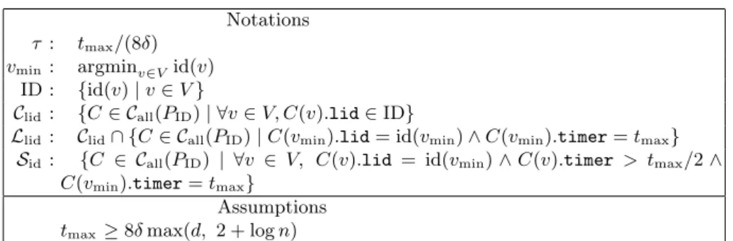
(6) Protocol 1 Leader Election with Identifiers PID Variables of each agent: lid ∈ I, timer ∈ [0, tmax ] Output function O: if v.lid = id(v) holds, then the output of agent v is L; Otherwise, F . Interaction between initiator x and responder y: 1: if x.lid > id(x) then x.lid ← id(x) endif 2: if x.lid < y.lid then 3: y.lid ← x.lid 4: x.timer ← y.timer ← max(x.timer − 1, 0) 5: else if x.lid > y.lid then 6: x.lid ← y.lid 7: x.timer ← y.timer ← max(y.timer − 1, 0) 8: else // x.lid = y.lid at this time 9: x.timer ← y.timer ← max(x.timer − 1, y.timer − 1, 0) 10: end if 11: if id(x) = x.lid or id(y) = y.lid then // a leader resets timers 12: x.timer ← y.timer ← tmax 13: else if x.timer = 0 then // a new leader is created at timeout 14: x.lid ← y.lid ← min(id(x), id(y)) 15: x.timer ← y.timer ← tmax 16: end if. Complexity Analysis The upper bound tmax of variable timer is the only parameter of PID , which affects the correctness and complexities of the protocol. We assume tmax ≥ 8δ max(d, 2+log n) where δ is the maximum degree of the agents and d is the diameter of population G. (Note that δ is an even number because G is undirected. ) We prove the following equations under this assumption: maxC∈Call ECTPID (C, Sid ) = O(mδτ log n), minC∈Sid EHTPID (C, LE ) = Ω(τ eτ ),. (1) (2). where τ = tmax /(8δ) and Sid is the set of configurations in which v.lid = id(vmin ) and v.timer > tmax /2 hold for all v ∈ V and vmin .timer = tmax holds. When upper bounds N of n and ∆ of δ are available and we assign tmax = 8N ∆, protocol PID is an (O(m∆N log n), Ω(N eN ))-loosely-stabilizing leader election protocol. First, we analyze the expected holding time. Let C0 ∈ Sid and ΞPID (C0 ) = C0 , C1 , . . . . To prove (2), it suffices to show that both C0 , . . . , C2mτ ∈ LE and C2mτ ∈ Sid hold with probability at least psuc = 1 − O(ne−τ ). Then, we have minC0 ∈Sid EHTPID (C0 , LE ) ≥ 2mτ /(1 − psuc ) = Ω(τ eτ ). Note We use some variants of Chernoff bounds for the proofs of Sections 3 and 4. See appendix for those Chernoff bounds. Lemma 1 The probability that every v ∈ V joins only less than tmax /2 interactions among Γ0 , . . . , Γ2mτ −1 is at least 1 − ne−τ ..

(7) Proof For any v ∈ V and t ≥ 0, v joins interaction Γt with probability at most δ/m. Thus, the number of interactions v joins during the 2mτ interactions is bounded by binomial random variable X ∼ B(2mτ, δ/m). Applying a variant of Chernoff bound (See Lemma C1 in Appendix), we have Pr(X ≥ tmax /2) = Pr(X ≥ 2E[X]) ≤e. = e−2δτ /3 ≤e. ∵ tmax = 8δτ. −E[X]/3. −τ. (By Chernoff Bound of Lemma C1) ∵δ≥2. .. Summing up the probabilities for all v ∈ V gives the lemma.. ⊓ ⊔. Lemma 2 Let C0 ∈ Llid and ΞPID (C0 ) = C0 , C1 , . . . . Then, we have the following inequality: Pr(∀v ∈ V, C2mτ (v).timer > tmax /2) ≥ 1 − 2ne−τ . Proof It suffices to show Pr(C2mτ (v).timer > tmax /2) ≥ 1 − 2e−τ for any agent v ∈ V . We denote the shortest path from vmin to v by (v0 , v1 , . . . , vk ) where v0 = vmin , vk = v, 0 ≤ k ≤ d and (vi−1 , vi ) ∈ E for all i = 1, . . . , k. For any t ∈ [0, 2mτ ], we define vhead (t) as vl with maximum l ∈ [1, k] such that there exist t1 , t2 , . . . , tl satisfying 0 ≤ t1 < t2 < · · · < tl < t and Γti ∈ {(vi−1 , vi ), (vi , vi−1 )} for i = 1, 2, . . . , l. We define vhead (t) = v0 if such l does not exist. Intuitively, vhead (t) is the head of the agents in path (v0 , v1 , . . . , vk ) to which a large timer value is propagated from vmin . (Remember that vmin resets the timers to tmax .) We define J(t) as the number of integers i ∈ [0, t] such that vhead (i) joins interaction Γi . Intuitively, J(t) is the number of interactions that the head agent joins among Γ0 , . . . , Γt . Obviously, we have Ct (vhead (t)).timer ≥ tmax − J(t) for any t ≥ 0. In what follows, we prove Pr(vhead (2mτ ) = v) ≥ 1 − e−τ and Pr(J(2mτ ) < tmax /2) ≥ 1 − e−τ , which give Pr(C2mτ (v).timer > tmax /2) ≥ 1 − 2e−τ . For any i ∈ [1, k], a pair vi−1 and vi interacts with probability 2/m at each interaction. Hence, we can say each interaction makes vhead forward with probability 2/m. Therefore, by letting Z be a binomial random variable such that Z ∼ B(2mτ, 2/m), we have Pr(vhead (t) = v) = 1 − Pr(Z < k) ≥ 1 − Pr(Z < d) ( ) 1 ≥ 1 − Pr Z < · E[Z] 4 ≥ 1 − e−9E[Z]/32 >1−e. −τ. ∵d≤τ =. 1 · E[Z] 4. (By Chernoff bound of Lemma C3). .. The probability that vhead (t) joins interaction Γt is at most δ/m regardless of t. Hence, by letting Z ′ be a binomial random variable such that Z ′ ∼ B(2mτ, δ/m),.

(8) we have Pr(J(2mτ ) < tmax /2) > 1 − Pr(Z ′ ≥ tmax /2) = 1 − Pr(Z ′ ≥ 2E[Z ′ ]) > 1 − e−E[Z =1−e. ′. ]/3. (By Chernoff bound of Lemma C1). −2δτ /3. > 1 − e−τ .. ∵δ≥2. Thus, we have shown Pr(C2mτ (v).timer > tmax /2) ≥ 1 − 2e−τ .. ⊓ ⊔. Lemma 3 minC∈Sid EHTPID (C, LE ) = Ω(τ eτ ). Proof We have C0 , . . . , C2mτ ∈ LE and C2mτ ∈ Sid if C0 ∈ Sid holds, no timeout happens, and any agent interacts at most tmax /2 times during 2mτ interactions. Hence, probability psuc discussed in the beginning of this section is at least 1 − 3ne−τ by Lemmas 1 and 2, which leads to the lemma. ⊓ ⊔ Next, we analyze the expected convergence time. To prove (1), we define two sets of configurations: Clid = {C ∈ Call (PID ) | ∀v ∈ V, C(v).lid ∈ ID} and Llid = Clid ∩ {C ∈ Call (PID ) | C(vmin ).lid = id(vmin ) ∧ C(vmin ).timer = tmax }. Lemma 4 maxC∈Call (PID ) ECTPID (C, Clid ) = O(mδτ log n). Proof Let z be the maximum value of v.timer such that v.lid ∈ / ID. This z decreases by one every time all interactions of E occur. Thus, it takes at most m m m m + m−1 + . . . 1 ≤ m(1 + log m) expected steps to decrease z by one. Hence, maxC∈Call (PID ) ECTPID (C, Clid ) ≤ tmax m(1 + log m) = O(mδτ log n). ⊓ ⊔ Lemma 5 maxC∈Clid ECTPID (C, Llid ) = O(m). Proof We have vmin .lid = id(vmin ) and vmin .timer = tmax just after vmin interacts in any configuration of Clid . This takes O(m) expected interactions. ⊓ ⊔ Lemma 6 maxC∈Llid ECTPID (C, Sid ) = O(mτ ). Proof Sketch Let C0 ∈ Llid and ΞPID (C0 ) = C0 , C1 , . . . . By similar argument to Lemmas 1 and 2, we can prove Pr(C2mτ ∈ Sid ) > 1 − 2ne−τ . Since C ∈ Llid cannot change to D ∈ / Llid , we have maxC∈Llid ECTPID (C, Sid ) ≤ 2mτ + 3ne−τ · maxC∈Llid ECTPID (C, Sid ). Solving this inequality gives the lemma. (See Appendix for the complete proof.) ⊓ ⊔ The following lemma immediately follows from Lemmas 4, 5, and 6. Lemma 7 maxC∈Call (PID ) ECTPID (C, Sid ) = O(mδτ log n). Lemmas 3 and 7 gives the following theorem. Theorem 1 Protocol PID is a (O(mδτ log n), Ω(τ eτ )) loosely-stabilizing leader election protocol for arbitrary graphs when tmax ≥ 8δ max(d, 2 + log n). Therefore, given upper bound N and ∆ of n and δ respectively, we get a (O(m∆N log n), Ω(N eN )) loosely-stabilizing leader election protocol for arbitrary graphs by assigning tmax = 8N ∆..

(9) 4. Leader Election with Random Numbers. This section presents loosely-stabilizing leader election protocol PRD . It works on arbitrary undirected anonymous graphs with a random number generated at each interaction (Protocol 2). Random numbers are used in Line 11: When the protocol enters Line 11, the code is executed with probability p = 1/|R|. This is implemented as the code is executed only when a specific number is generated. For example, p = 0.01 if we assign R = [0, 99] and treat 0 as a specific number. Each agent has binary variable DoA ∈ {DEAD, ALIVE} and three timers timerL , timerV and timerS . The output function defines leaders based on DoA : agent v is a leader if v is alive (or v.DoA = ALIVE), and a follower if v is dead (or v.DoA = DEAD). Protocol PRD consists of a timeout mechanism (Lines 1-7) and a virus-war mechanism (Lines 8-14). By using timerL , the timeout mechanism creates a leader when it is suspected that no leader exists. By using timerV and timerS , the virus-war mechanism reduces the number of leaders. The timeout mechanism is almost the same as PID . By the timer reset and the larger value propagation, timeout eventually occurs when no leader exists, and all agents keep high timer values with high probability when one ore more leaders exist. At timeout, a dead agent becomes a leader (Line 5). In the virus-war mechanism, each leader tries to kill other leaders by viruses and become the unique leader. We say that agent v has a virus if v.timerV > 0, and v wears a (head) shield if v.timerS > 0. A leader creates a new virus with probability p when it interacts as an initiator (Line 11). When creating a virus, the agent wears a shield so as not to be killed by the new virus (Line 11). A virus spreads among agents by interactions (Line 8), and an agent is killed when it has a virus without a shield (Lines 13-14). A virus has TTL (time to live), which is memorized on timerV and decreased by one at each interaction of its owner (line 8). When timerV becomes zero, the virus vanishes and looses the ability to kill agents. A shield also has TTL, which is memorized on timerS and decreased by one at each interaction of its owner (Line 9). When timerS becomes zero, the shield vanishes and looses the ability to protect its owner from viruses. The virus-war mechanism correctly works if p is sufficiently small and tshld is sufficiently greater than tvirus . Consider the case multiple leaders exist. Since p is small, all viruses and shields eventually vanishes. After that, some agent eventually creates a new virus and shield. The created virus kill all other agents unless some of them also create a new virus and shield before the virus reaches them. Since p is sufficiently small, the probability of the latter is small. Thus, the unique leader is elected within a relatively short time. Even after that, the unique leader keeps on creating new viruses, each of which may kill the leader. However, the leader is not killed for an extremely long time: since tshld ≫ tvirus , the leader’s shield rarely vanishes before all viruses vanish from the population. Complexity Analysis We have four parameters in PRD : three upper bounds tmax , tvirus , and tshld of the timers, and probability p. We assume tvirus = tmax /2, tmax ≥ 8δ max(d, 2 + log(13nδ⌈log n⌉)), tshld ≥ 2δtmax ⌈log n⌉ and p ≤.

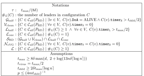
(10) Protocol 2 Leader Election with Random Numbers PRD Variables of each agent: DoA ∈ {DEAD, ALIVE}, timerL ∈ [0, tmax ], timerV ∈ [0, tvirus ], timerS ∈ [0, tshld ] Output function O: if v.DoA = ALIVE holds, then the output of agent v is L, otherwise F . Interaction between initiator x and responder y: 1: x.timerL ← y.timerL ← max(x.timerL − 1, y.timerL − 1, 0) 2: if x.DoA = ALIVE or y.DoA = ALIVE then 3: x.timerL ← y.timerL ← tmax // a leader resets timer 4: else if x.timerL = 0 then // a new leader is created at timeout 5: x.DoA ← ALIVE 6: x.timerL ← y.timerL ← tmax 7: end if 8: x.timerV ← y.timerV ← max(x.timerV − 1, y.timerV − 1, 0) 9: x.timerS ← max(0, x.timerS − 1) 10: if x.DoA = ALIVE then 11: Execute (x.timerS ← tshld , x.timerV ← tvirus ) with probability p 12: end if 13: if x.timerV > 0 and x.timerS = 0 then x.DoA ← DEAD endif 14: if y.timerV > 0 and y.timerS = 0 then y.DoA ← DEAD endif. (4mtshld )−1 . We prove the following equations under this assumption: maxC∈Call ECTPRD (C, SRD ) = O(mp−1 ), minC∈SRD EHTPRD (C, LE ) = Ω(τ eτ ),. (3) (4). where τ = tmax /(8δ) and SRD is the set of configurations we define later. When upper bounds N and ∆ are available and we assign tmax = 8N ∆, tshld = 2∆tmax ⌈log N ⌉ and p = (4N 2 tshld )−1 (i.e., R = [0, 4N 2 tshld − 1]), then PRD is an (O(m∆2 N 3 log N ), Ω(N eN ))-loosely-stabilizing leader election protocol. Before proving equations (3) and (4), we define five sets of configurations: Ghalf = {C ∈ Call (PRD ) | ∃v ∈ V, C(v).DoA = ALIVE ∧ C(v).timerS > tshld /2}, Vclean = {C ∈ Call (PRD ) | ∀v ∈ V, C(v).timerV = 0}, Lhalf = {C ∈ Call (PRD ) | #L (C) ≥ 1 ∧ ∀v ∈ V, C(v).timerL > tmax /2}, Lone = {C ∈ Call (PRD ) | #L (C) = 1}, SRD = (Ghalf ∪ Vclean ) ∩ Lhalf ∩ Lone , where #L (C) denotes the number of leaders in configuration C. Note that Ghalf requires that not all agents but at least one leader has timerS more than tshld /2. First, we analyze the expected holding time. Let C0 ∈ SRD and ΞPRD (C0 ) = C0 , C1 , . . . . To prove (4), it suffices to show that both C0 , . . . , C8mδτ ⌈log n⌉ ∈ LE and C8mδτ ⌈log n⌉ ∈ SRD hold with probability no less than psuc = 1 − O(nδ log n · e−τ ). Then, minC0 ∈SRD EHTPRD (C0 , LE ) ≥ 8mδτ ⌈log n⌉τ /(1 − psuc ) = Ω(τ eτ ). We define two predicates PROPi and HALFi for any i ≥ 0: PROPi = 1 if C2mτ (i+1) (v).timerL > ti − tmax /2 for all v ∈ V , otherwise PROPi = 0, where.

(11) ti = maxv∈V C2mτ i (v); HALFi = 1 if every agent joins only less than tmax /2 interactions among Γ2mτ i , . . . , Γ2mτ (i+1)−1 , otherwise HALFi = 0. Intuitively, PROPi = 1 means the maximum value of timerL propagates to all the agents well during the 2mτ interactions, and HALFi = 1 means every agent does not interact so much during the 2mτ interactions. Lemma 8 Let C0 ∈ SRD and ΞPRD (C0 ) = C0 , C1 , . . . . Then, we have both C0 , . . . , C8mδτ ⌈log n⌉ ∈ LE and C8mδτ ⌈log n⌉ ∈ SRD if the following conditions hold: (A) #L (Ct ) ≥ 1 for all t = 0, . . . , 8mδτ ⌈log n⌉, (B) C8mδτ ⌈log n⌉ ∈ Ghalf ∪ Vclean , (C) PROPi = 1 for all i = 0, . . . , 4δ⌈log n⌉ − 1, and (D) HALFi = 1 for all i = 0, . . . , 4δ⌈log n⌉ − 1. Proof We have C2mτ i (v).timerL > tmax /2 for any i ∈ [0, 4δ⌈log n⌉] from (A) and (C). Since no agent interacts more than tmax /2 times among each 2mτ interactions (i.e. (D)), timeout does not occur at any interaction Γ0 , . . . , Γ8mδτ ⌈log n⌉−1 , by which we obtain C0 , . . . , C8mδτ ⌈log n⌉ ∈ LE . We also obtain C8mδτ ⌈log n⌉ ∈ Lhalf ∩ Lone ∩ (Ghalf ∪ Vclean ) = SRD from above discussion and (B). ⊓ ⊔ Lemma 9 The probability that every agent joins only less than tshld /2 interactions as an initiator among Γ0 , . . . , Γ8mδτ ⌈log n⌉−1 is at least 1 − ne−δτ . Proof For any v ∈ V and t ≥ 0, v joins interaction Γt as an initiator with probability at most δ/(2m) since v has at most δ/2 outgoing edges. Thus, the number of interactions v joins as an initiator during the 8mδτ ⌈log n⌉ interactions is bounded by binomial random variable X ∼ B(8mδτ ⌈log n⌉, δ/(2m)). We have Pr(X ≥ tshld /2) ≤ Pr(X ≥ 8δ 2 τ ⌈log n⌉) = Pr(X ≥ 2E[X]) ≤ e−E[X]/3 =e. ∵ tshld ≥ 16δ 2 τ ⌈log n⌉. (By Chernoff Bound of Lemma C2). −4δ 2 τ ⌈log n⌉/3. = e−δτ . Summing up these probabilities gives the lemma.. ⊓ ⊔. Lemma 10 Let C0 ∈ SRD and ΞPRD (C0 ) = C0 , C1 , . . . . Then, we have Pr(∀t ∈ [0, 8mδτ ⌈log n⌉ − 1], #L (Ct ) ≥ 1) ≥ 1 − ne−δτ . Proof By Lemma 9, it suffices to show that #L (Ct ) ≥ 1 holds for all t ∈ [0, 8mδτ ⌈log n⌉] when we assume every agent joins only less than tshld /2 interactions as an initiator among Γ0 , . . . , Γ8mδτ ⌈log n⌉−1 . Since C0 ∈ SRD , we have C0 ∈ Ghalf ∪Vclean . If C0 ∈ Ghalf , there exists a leader v such that C0 (v).timerS > tshld /2. By the assumption, v decrease its timerS by at most tshld /2; thus, v is never killed and remains a leader in C0 , . . . , C8mδτ ⌈log n⌉ . If C0 ∈ Vclean , no leader is killed before a new virus is created. Even if some leader u creates a new virus at interaction Γt (0 ≤ t < 8mδτ ⌈log n⌉), u wears a new shield at the same time. Hence, u remains a leader in Ct , . . . , C8mδτ ⌈log n⌉ by the assumption. ⊓ ⊔.

(12) We define the first round time RTΓ (1) as the minimum t satisfying ∀e ∈ E, 0 ≤ ∃t′ ≤ t, Γt′ = e. For any i ≥ 2, we define the i-th round time RTΓ (i) as the minimum t satisfying ∀e ∈ E, RTΓ (i − 1) < ∃t′ ≤ t, Γt′ = e. Lemma 12 bounds RTΓ (i) from above with high probability. To prove the lemma, we firstly prove Lemma 11. Lemma 11 Let v1 , v2 , . . . , vl be any l (l < n) agents in V . There exists at least 2l edges of E that are incident to at least one of the l agents. Proof Since l < n, there exists agent r ∈ V that differs from any v1 , v2 , . . . , vl . Since G is strongly connected, there exists a rooted spanning tree T on G where r is the root agent of T . Then, every vi (i ∈ [1, k]) has two edges between vi and the parent agent of vi in T . (Remind that G is undirected, that is, (u, v) ∈ E ⇔ (v, u) ∈ E for any u, v ∈ V .) These edges are mutually exclusive. Thus, we have 2l edges of E that are incident to at least one of the l agents. ⊓ ⊔ Lemma 12 Pr(RTΓ (i) < 2im⌈log n⌉) ≥ 1 − ne−i/4 holds for any i ≥ 1. Proof Each round j (j ≥ 1) finishes when every agent v ∈ V interacts in round j. Consider the case that k (k ≥ 1) agents have not yet interacted in round j and only n−k agents have interacted in round j. We call the former uninvolved agents and the latter involved agents. If k < n, one of the k uninvolved agents joins the next interaction and becomes an involved agent with probability more than 2k/m by Lemma 11. If k = n, some uninvolved agent joins the next interaction with probability 1. Let Xj,k (j ≥ 1, k ≥ 1) be the random variable that corresponds to the number of trials to the first success in which the success probability of each trial is 2k/m. From the above discussion, we obtain   ( ) i n−1 ∑ ∑ Pr(RTΓ (i) ≥ 2im⌈log n⌉) ≤ Pr  1+ Xj,k ≥ 2im⌈log n⌉  ≤ Pr . j=1 n−1 i ∑∑. k=1. . (5). Xj,k ≥ 2im⌈log n⌉ − i .. k=1 j=1. ∑i 2k For binomial random variable Yk ∼ B(⌈ im j=1 Xj,k > k ⌉, m ), we have Pr( ∑i im Pr( j=1 Xj,k ≥ ⌈ k ⌉) ≤ Pr(Yk ≤ i). Hence, we have  Pr . i ∑ j=1. Xj,k. im k ).  im  > ≤ Pr(Yk ≤ i) k ) ( 1 ≤ Pr Yk ≤ · E[YK ] 2 ≤ e−E[Yk ]/8 −i/4. ≤e. .. (By Chernoff Bound of Lemma C2). ≤. (6).

(13) From Inequalities (5) and (6), we have . . Pr(RTΓ (i) ≥ 2im⌈log n⌉) ≤ Pr . Xj,k ≥ 2im⌈log n⌉ − i. n−1 i ∑∑. . k=1 j=1. n−1 i ∑∑. ≤ Pr . Xj,k. k=1 j=1. ≤. n−1 ∑. . Pr . k=1. i ∑. Xj,k. j=1.  im  > k k=1  im  > k n−1 ∑. ≤ ne−i/4 , ∑n−1 where k=1 im k ≤ im(1 + log n) − i < 2im⌈log n⌉ − i is used for the second inequality. Thus, Pr(RTΓ (i) < 2im⌈log n⌉) ≥ 1 − ne−i/4 holds. ⊓ ⊔ Lemma 13 Let C0 ∈ SRD and ΞPRD (C0 ) = C0 , C1 , . . . . Then, we have Pr(C8mδτ ⌈log n⌉ ∈ Ghalf ∪ Vclean ) ≥ 1 − 2ne−δτ . Proof Assume that RTΓ (tvirus ) < 8mδτ ⌈log n⌉ holds and every agent joins only less than tshld /2 interactions as an initiator among Γ0 , . . . , Γ8mδτ ⌈log n⌉−1 . These assumptions lead to C8mδτ ⌈log n⌉ ∈ Ghalf ∪ Vclean as follows. If a new virus is not created among Γ0 , . . . , Γ8mδτ ⌈log n⌉−1 , then all viruses in the initial configuration vanish during the period since each round decreases the maximum value of timerV by at least one. Thus, C8mδτ ⌈log n⌉ ∈ Vclean holds. If some agent v creates a new virus at Γt , then v wears a new shield at the same time. Thus, Ct+1 (v).timerS = tshld . Since v interacts as an initiator only less than tshld /2 times among Γt+1 , . . . , Γ8mδτ ⌈log n⌉−1 , we have C8mδτ ⌈log n⌉ (v).timerS > tshld /2, which means C8mδτ ⌈log n⌉ ∈ Ghalf . By tvirus = 4δτ and Lemmas 9 and 12, the probability that the two assumptions hold is at least 1 − 2ne−δτ . ⊓ ⊔ Lemma 14 Pr(PROPi = 1) ≥ 1 − 2ne−τ for any i ≥ 0. Proof The same argument as the proof of Lemma 2 gives the lemma.. ⊓ ⊔. Lemma 15 Pr(HALFi = 1) ≥ 1 − ne−τ for any i ≥ 0. Proof Each interaction is independent. Thus, Lemma 1 gives the lemma.. ⊓ ⊔. Lemma 16 minC∈SRD EHTPRD (C, LE ) = Ω(τ eτ ). Proof Probability psuc , discussed in the beginning of this section, is at least 1 − 3ne−δτ − 4δ⌈log n⌉ · 3ne−τ ≥ 1 − 13nδ⌈log n⌉e−τ by Lemmas 8, 10, 13, 14 and 15, which leads to the lemma. ⊓ ⊔ Next, we analyze the expected convergence time. We define two sets of configurations: NoVG = {C ∈ Call (PRD ) | ∀v ∈ V, C(v).timerV = C(v).timerS = 0} and L = {C ∈ Call (PRD ) | #L (C) ≥ 1}..

(14) Lemma 17 maxC∈Call (PRD ) ECTPRD (C, SRD ) = O(mp−1 ). Proof Sketch Probability p, with which a leader creates a virus at each interaction, is sufficiently small (p < 1/(4mtshld )). Thus, the probability that all viruses and shields vanish (i.e. the population enters a configuration of NoVG ) within 2mtshld interactions is at least 1−(2mtshld ·p+O(ne−τ )) > 1/2−O(ne−τ ). Even if the reached configuration of NoVG does not have any leader, the timeout mechanism creates a leader, and the population enters a configuration of NoVG ∩ L. This takes less than 16mδτ ⌈log n⌉ interactions with probability 1 − O(ne−τ ). After the population enters into NoVG ∩L, additional ⌈m/p⌉ interactions create a new virus with probability 1−e−2 . Let v be a leader that creates the virus. Since v wears a new shield at the same time, v is not killed and remains a leader during the next 2mτ interactions with probability 1 − O(e−τ ). On the other hand, the virus spreads to all the agents within these 2mτ interactions with probability 1−O(ne−τ ), killing all the agents other than v. A leader other than v may create a new virus during the 2mτ interactions, and survives with a shield. However, this probability is at most 2mτ · p ≤ 1/4. Hence, v becomes the unique leader within the 2mτ interactions with probability 3/4−O(ne−τ ). After the 2mτ interactions, all the agents have timerL > tmax /2 with probability 1 − O(ne−τ ) by the larger value propagation, and v.timerS > tshld /2 holds with probability 1 − O(ne−τ ). Hence, the population enters a configuration of Lone ∩ Lhalf ∩ Ghalf ⊂ SRD within the 2mτ interactions with probability 3/4 − O(ne−τ ). As a result, starting from any configuration, the population enters into SRD within O(mp−1 ) interactions with probability 1/4 − e−2 − O(ne−τ ) > 0.11 − o(1), which gives the lemma. (See Appendix for the complete proof.) ⊓ ⊔ Lemmas 16 and 17 gives the following theorem. Theorem 2 Protocol PRD is a (O(mp−1 ), Ω(τ eτ )) loosely-stabilizing leader election protocol for arbitrary graphs when tmax ≥ 8δ max(d, 2 + log(13nδ⌈log n⌉)), tvirus = tmax /2, tshld ≥ 2δtmax ⌈log n⌉ and p ≤ (4mtshld )−1 . Therefore, given upper bound N and ∆ of n and δ respectively, we get a (O(m∆2 N 3 log N ), Ω(N eN )) loosely-stabilizing leader election protocol for arbitrary graphs by assigning tmax = 8N ∆, tvirus = tmax /2, tshld = 2∆tmax ⌈log N ⌉ and p = (4N 2 tshld )−1 .. 5. Conclusion. We have presented two loosely-stabilizing leader election protocols for arbitrary undirected graphs in the PP model: one works with agent-identifiers and the other works with random numbers. Both protocols keep a unique leader for an exponentially long expected time after entering a loosely-safe configuration. The protocols use only upper bounds N of n and ∆ of δ while any self-stabilizing leader election protocol needs the exact knowledge of n. The restriction of the protocols to undirected graph is only for simplicity of protocol description and.

(15) complexity analysis. The proposed protocols also work on arbitrary directed graphs with slight modification: it is only necessary that a responder also executes some actions of an initiator (Line 1 of Protocol 1 and Lines 10-12 of Protocol 2). Our future work is to develop a loosely-stabilizing leader election protocol without agent-identifiers or random numbers for arbitrary graphs. We will also tackle with loosely-stabilizing leader election for some classes of graphs (e.g. rings and trees).. References 1. D. Angluin, J Aspnes, Z. Diamadi, M.J. Fischer, and R. Peralta. Computation in networks of passively mobile finite-state sensors. Distributed Computing, 18(4):235– 253, 2006. 2. D. Angluin, J. Aspnes, and D. Eisenstat. fast computation by population protocols with a leader. In DISC, pages 61–75, 2006. 3. D. Angluin, J. Aspnes, M. J Fischer, and H. Jiang. Self-stabilizing population protocols. ACM Transactions on Autonomous and Adaptive Systems, 3(4):13, 2008. 4. J. Beauquier, P. Blanchard, and J. Burman. Self-stabilizing leader election in population protocols over arbitrary communication graphs. In OPODIS, pages 38–52, 2013. 5. J. Beauquier, J. Burman, L. Rosaz, and B. Rozoy. Non-deterministic population protocols. In OPODIS, pages 61–75, 2012. 6. S. Cai, T. Izumi, and K. Wada. How to prove impossibility under global fairness: On space complexity of self-stabilizing leader election on a population protocol model. Theory of Computing Systems, 50(3):433–445, 2012. 7. D. Canepa and M. G. Potop-Butucaru. Stabilizing leader election in population protocols. 2007. http://hal.inria.fr/inria-00166632. 8. M. J. Fischer and H. Jiang. Self-stabilizing leader election in networks of finite-state anonymous agents. In OPODIS, pages 395–409, 2006. 9. R. Guerraoui and E. Ruppert. Even small birds are unique: Population protocols with identifiers. Rapport de Recherche CSE-2007-04, Department of Computer Science and Engineering, York University, York, ON, Canada, 2007. 10. O. Michail, I. Chatzigiannakis, and P. G. Spirakis. Mediated population protocols. Theoretical Computer Science, 412(22):2434–2450, 2011. 11. M. Mitzenmacher and E. Upfal. Probability and Computing: Randomized Algorithms and Probabilistic Analysis. Cambridge University Press, 2005. 12. R. Mizoguchi, H. Ono, S. Kijima, and M. Yamashita. On space complexity of selfstabilizing leader election in mediated population protocol. Distributed Computing, 25(6):451–460, 2012. 13. Y. Sudo, J. Nakamura, Y. Yamauchi, F. Ooshita, H. Kakugawa, and T. Masuzawa. Loosely-stabilizing leader election in a population protocol model. Theoretical Computer Science, 444:100–112, 2012. 14. X. Xu, Y. Yamauchi, S. Kijima, and M. Yamashita. Space complexity of selfstabilizing leader election in population protocol based on k-interaction. In SSS, pages 86–97, 2013..

(16) Table 1. Notations and Assumptions for PID. τ : vmin : ID : Clid : Llid : Sid :. Notations tmax /(8δ) argminv∈V id(v) {id(v) | v ∈ V } {C ∈ Call (PID ) | ∀v ∈ V, C(v).lid ∈ ID} Clid ∩ {C ∈ Call (PID ) | C(vmin ).lid = id(vmin ) ∧ C(vmin ).timer = tmax } {C ∈ Call (PID ) | ∀v ∈ V, C(v).lid = id(vmin ) ∧ C(v).timer > tmax /2 ∧ C(vmin ).timer = tmax } Assumptions tmax ≥ 8δ max(d, 2 + log n). Appendix The appendix presents the proofs of the lemmas that have only proof sketches in the main body of this paper. Specifically, we presents the complete proofs of Lemmas 6 and 17 in Sections A and B respectively. In Section C, we show the three variants of Chernoff bounds [11] used in several proofs of this paper. The appendix also presents Tables 1 and 2 that summarize notations and assumptions for protocols PID and PRD respectively.. A. Proofs in Leader Election with Identifiers. Lemma 6 maxC∈Llid ECTPID (C, Sid ) = O(mτ ). Proof Let C0 ∈ Llid and ΞPID (C0 ) = C0 , C1 , . . . . Since Ct ∈ Llid holds for every t ≥ 0, identifier id(vmin ) is the smallest among lid of all the agents in any configuration C0 , C1 , . . . . Hence, once agent v satisfies v.lid = id(vmin ), then v.lid = id(vmin ) always holds until a timeout occurs at v. Lemma 2 has shown that, with probability at least 1 − 2ne−τ , every agent v satisfies v.lid = id(vmin ) within 2mτ interactions, and after that, keeps on satisfying v.timer > tmax /2 at least until Γ2mτ −1 finishes. Thus, the probability that C2mτ (v).lid = id(vmin ) and C2mτ (v).timer > tmax /2 hold for all v ∈ V is at least 1 − 2ne−τ . Note that C2mτ (vmin ).timer = tmax holds with probability 1. Hence, we have max ECTPID (C, Sid ) ≤ 2mτ + 2ne−τ · max ECTPID (C, Sid ).. C∈Llid. C∈Llid. Solving this inequality gives maxC∈Llid ECTPID (C, Sid ) ∈ O(mτ ).. B. ⊓ ⊔. Proofs in Leader Election with Random Numbers. We show Lemmas B2, B3 and B5 to prove Lemma 17. Lemma B2 (B3, B5) gives the lower bound of the probability that the population enters from Call (PRD ).

(17) Table 2. Notations and Assumptions for PRD. τ #L (C) Ghalf Vclean Lhalf Lone SRD NoVG L. : : : : : : : : :. Notations tmax /(8δ) the number of leaders in configuration C {C ∈ Call (PRD ) | ∃v ∈ V, C(v).DoA = ALIVE ∧ C(v).timerS > tshld /2} {C ∈ Call (PRD ) | ∀v ∈ V, C(v).timerV = 0} {C ∈ Call (PRD ) | #L (C) ≥ 1 ∧ ∀v ∈ V, C(v).timerL > tmax /2} {C ∈ Call (PRD ) | #L (C) = 1} (Ghalf ∪ Vclean ) ∩ Lhalf ∩ Lone {C ∈ Call (PRD ) | ∀v ∈ V, C(v).timerV = C(v).timerS = 0} {C ∈ Call (PRD ) | #L (C) ≥ 1} Assumptions tmax ≥ 8δ max(d, 2 + log(13nδ⌈log n⌉)) tvirus = tmax /2 tshld ≥ 2δtmax ⌈log n⌉ p ≤ (4mtshld )−1. into NoVG (from NoVG into NoVG ∩ L, from NoVG ∩ L into SRD , respectively) within a certain number of interactions. We also show Lemmas B1 and B4 to prove Lemmas B2 and B5 respectively. Lemma B1 The probability that every v ∈ V joins more than tshld interactions as an initiator among Γ0 , . . . , Γ2mtshld is at least 1 − ne−tshld /4 . Proof For any v ∈ V and t ≥ 0, v joins interaction Γt as an initiator with probability at least 1/m. Thus, the number of interactions v joins during the 2mtshld interactions is bounded from below by binomial random variable X ∼ B(2mtshld , 1/m). Applying the Chernoff bound of Lemma C2, we have Pr(X ≤ tshld ) = Pr(X ≤ E[X]/2) ≤ e−E[X]/8 =e. −tshld /4. (By Chernoff Bound of Lemma C2). .. Summing up the probabilities for all v ∈ V gives the lemma.. ⊓ ⊔. Lemma B2 Let C0 ∈ Call (PRD ) and ΞPRD (C0 ) = C0 , C1 , . . . . Then, we have Pr(C2mtshld ∈ NoVG ) ≥ 1 − 2ne−δτ − 2mtshld · p. Proof First, we show that C2mtshld ∈ NoVG holds when the following three conditions hold: (A) every agent v ∈ V joins more than tshld interactions as an initiator among Γ0 , . . . , Γ2mtshld , (B) RT(tvirus ) ≤ 2mtshld , and (C) no new virus is created during Γ0 , . . . , Γ2mtshld ..

(18) Until a new virus is created, variable v.timerS for each v ∈ V is monotonically non-increasing and it decreases by one every time v interacts as an initiator. Hence, no agent wears a shield in configuration C2mtshld by (A) and (C). Until a new virus is created, the maximum value of all v.timerV (i.e. maxv∈V v.timerV ) is monotonically non-increasing during Γ0 , . . . , Γ2mtshld and it decreases at least by one in each round. Hence, no agent has a virus in configuration C2mtshld by (B) and (C). Thus, we have C2mtshld ∈ NoVG when (A),(B) and (C) hold. Next we give lower bounds on probability of (A),(B) and (C). The probability of (A) is at least 1 − ne−tshld /4 > 1 − ne−δτ from Lemma B1. The probability of (B) is at least 1 − ne−tvirus /4 = 1 − ne−δτ from Lemma 12. At each interaction, a new virus is created with probability at most p (with probability exact p when a leader interacts as an initiator and with probability 0 otherwise). Hence, the probability of (C) is at least 1 − 2mtshld · p. Thus, Conditions (A),(B) and (C) hold with probability at least 1 − 2ne−δτ − 2mtshld · p. ⊓ ⊔ Lemma B3 Let C0 ∈ NoVG and ΞPRD (C0 ) = C0 , C1 , . . . . Then, we have Pr(∃i ∈ [0, 16mδτ ⌈log n⌉], Ci ∈ NoVG ∩ L) ≥ 1 − 2ne−δτ . Proof The lemma trivially holds if C0 has one or more leaders. Therefore, we consider the case C0 does not have any leader (i.e. C0 ∈ / L). Since followers never create viruses or shields, there exists neither a virus nor a shield until a leader is created. Therefore, the population reaches a configuration of NoVG ∩ L at the first timeout of execution ΞPRD (C0 ) = C0 , C1 , . . . . Thus, it suffices to show that a timeout occurs within 16mδτ ⌈log n⌉ interactions with probability at least 1 − 2ne−δτ . During the period no leader exists, the maximum value of all v.timerL (i.e. maxv∈V v.timerL ) is monotonically non-increasing and decreases at least by one in each round. This means a timeout occurs until tmax rounds finish. By Lemma 12, we have Pr(RT(tmax ) < 16mδτ ⌈log n⌉) ≥ 1 − ne−tmax /4 = 1 − ne−2δτ . ⊓ ⊔ Lemma B4 Let C0 ∈ Call (PRD ) and ΞPRD (C0 ) = C0 , C1 , . . . . Let tinit be the maximum value of all v.timerV in C0 (i.e. maxv∈V C(v).timerV ). Then, we have Pr(∀v ∈ V, C2mτ (v).timerV > tinit − tmax /2) > 1 − 2ne−τ . Proof The same argument as the proof of Lemma 2 gives the lemma.. ⊓ ⊔. Lemma B5 Let C0 ∈ NoVG ∩ L and ΞPRD (C0 ) = C0 , C1 , . . . . Then, we have Pr(∃i ∈ [0, ⌈2mp−1 ⌉ + 2mτ ], Ci ∈ SRD ) ≥ 1 − e−2 − 5ne−τ − 2mτ · p. Proof Let t be the minimum integer (i.e. the first time) such that configuration Ct has a virus. During the period one or more leaders exist, each interaction makes a new virus with probability at least p/m. Hence, the probability of −1 t < ⌈2mp−1 ⌉ is at least 1 − (1 − p/m)⌈2mp ⌉ > 1 − e−2 . Therefore, it suffices to show that Ct+2mτ ∈ SRD holds with probability at least 1 − 5ne−τ − 2mτ · p. We denote the leader that creates a virus at interaction Γt−1 by v. Note that, in configuration Ct , only v has a virus and a shield while the other agents do not have viruses or shields. Furthermore, the virus and the.

(19) shield of v have the maximum TTL (tvirus and tshld respectively in Ct . We have Ct+2mτ ∈ SRD if all the following conditions hold: (A) every agent has a virus in Ct+2mτ , (B) every agent except for v does not wear a shield in Ct+2mτ , (C) agent v joins only less than tshld /2 interactions as an initiator during Γt , Γt+1 , . . . , Γt+2mτ −1 , and (D) every agent has timerL larger than tmax /2 in Ct+2mτ . By (A) and (B), all agents except for v are dead in Ct+2mτ . By (C), v always has a shield larger than tshld /2 during the 2mτ interactions, and hence, is alive (i.e. is a leader) in Ct+2mτ . Therefore, Ct+2mτ ∈ Lone ∩ Ghalf holds. Moreover, Ct+2mτ ∈ Lhalf holds by (D). Thus, we have Ct+2mτ ∈ Lone ∩ Ghalf ∩ Lhalf ⊂ SRD when (A),(B),(C) and (D) hold. Therefore, it suffices to show that all (A),(B),(C) and (D) hold with probability 1 − 5ne−τ − 2mτ · p. Since Ct (v).timerV = tvirus = tmax /2, the probability of (A) is at least 1 − 2ne−τ by Lemma B4. The sufficient condition of (B) is that a new virus is not created during Γt , Γt+1 , . . . , Γt+2mτ −1 . The probability of this condition is at least 1 − 2mτ · p. The probability of (C) is at least 1 − ne−δτ > 1 − ne−τ by Lemma 9. Finally, The probability of (D) is at least 1 − 2ne−τ by Lemma 14. Thus, all (A), (B), (C) and (D) hold with probability at least 1 − 5ne−τ − 2mτ · p. ⊓ ⊔ Lemma 17 maxC∈Call (PRD ) ECTPRD (C, SRD ) = O(mp−1 ). Proof By Lemmas B2, B3 and B5, starting from any configuration of Call (PRD ), the population enters a configuration of SRD within 2mtshld + 16mδτ ⌈log n⌉ + ⌈2mp−1 ⌉ + 2mτ interactions with probability at least 1 − 2ne−δτ − 2mtshld · p − 2ne−δτ − e−2 − 5ne−τ − 2mτ · p. The former expression is at most ⌈(2m + 1) · p−1 ⌉ and the latter expression is at least 1 − 3mtshld · p − 6ne−τ − e−2 > 1 − 3/4 − 6e−2 /26 − e−2 > 0.08. Hence, we have max. ECTPRD (C, SRD ). C∈Call (PRD ). ≤ ⌈(2m + 1)p−1 ⌉ + 0.92 ·. max C∈Call (PRD ). ECTPRD (C, SRD ).. Solving this inequality gives maxC∈Call (PRD ) ECTPRD (C, SRD ) = O(mp−1 ).. C. ⊓ ⊔. Chernoff Bounds. Lemma C1 (from Eq. (4.2) in [11]) The following inequality holds for any binomial random variable X: Pr(X ≥ 2E[X]) ≤ e−E[X]/3 ..

(20) Lemma C2 (from Eq. (4.5) in [11]) The following inequality holds for any binomial random variable X: Pr(X ≤ E[X]/2) ≤ e−E[X]/8 . Lemma C3 (from Eq. (4.5) in [11]) The following inequality holds for any binomial random variable X: Pr(X ≤ E[X]/4) ≤ e−9E[X]/32 ..

(21)