Reception of the Jupiter Decameter Waves at
Mt.Zao Observatory
著者
Oya Hiroshi, Morioka Akira, Kondo Minoru
雑誌名
Science reports of the Tohoku University. Ser.
5, Geophysics
巻
22
号
3-4
ページ
137-144
発行年
1975-04
URL
http://hdl.handle.net/10097/44724
Sci. Rep, TOhoku Univ., Ser. 5, Geophysics, Vol. 22, Nos. 3-4 , pp. 137-143, 1975.
Reception of the Jupiter Decameter Waves at Mt.
Zao Observatory
HIROSHI OYA, AKIRA MORIOKA, and MINORU KONDO
Upper Atmosphere and Space Research Laboratory
TOhoku University, Katahira, Sendai 980, Japan
(Received January 11, 1975)
Abstract: A new station for the observation of Jovian decameter wave emissions
has been developed at Mt. Zao Observatory . Using the dipole antenna with
quarter wavelength elements, that is equipped with a reflector element, gives a threshold value, 10-21 Watt/m2Hz. From Oct. 20, 1974 , a succesful observation of the decameter wave emissions provides the data that give an identification of the main and the early sources of the emissions; it is also confirmed that the early source emissions are controlled by the position of Io satellite. The galactic decameter waves are also identified; the maximum value of the measured galactic intensity is 5 X 10-19 Wattim2Hz.
1. Introduction
After the first identification of the Jupiter decameter waves by Burke and Franklin (1955), the observations of the Jupiter decameter waves have been carried out extensively during last two decades. The observation stations, at Boulder (Warwick, 1967), Florida (Carr, 1961) and Greenbelt (Alexander, 1967) were established in USA and a station was built at Tasmania (Ellis, 1965) in Australia. The data provided by these stations were used to clarify the fundamental features of the Jupiter decameter waves. Being based on these established features, the mechanisms of the decameter wave origin were discussed but the origin of this decameter waves had not been settled yet. A new theory on the origin of the decameter waves has been presented (Oya, 1974). On this theory, the plasma waves are considered to be an origin; while the plasma waves propagate through the Jupiter plasmasphere, the plasma waves can be converted into the electromagnetic waves. The calculated conversion rate indicates high values within a range from 1 to 10%.
New data of the Jupiter decameter waves are required to investigate this proposed hypothesis. The data can also provide important informations on the Jupiter plasmasphere and the mangetosphere. For this motivation, a new observation station has been established at Mt. Zao Observatory of Upper Atmosphere and Space Research Laboratroy, Tohoku University, Sendai, Japan. The station has started to rec jive the decameter waves from October 20, 1974. This is a preliminary report of the development of the new decameter observation station. The contents are mainly concentrated to the technical side; a result of recent observation is given in the last part.
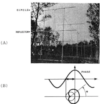
138 H. OYA, A. MORIOKA and M. KONDO (A) (B) DIPOL E-. REFLECTOR. ^ PHASE
Fig. 1. Antenna configuration (A) and the gain characteristics (B).
2. Antenna and Pre-Amplifier
The decameter waves are received at four frequencies as 19.945 MHz, 20.010 MHz, 23.505 MHz and 24.320 MHz using the dipole with quarter wave, length elements. As has been given in Fig. 1, this dipole is equipped with a set of reflector. The total antenna gain is approximately 4dB and indicates (1+ cos 0) relationship with resepct to the azimuth 0 (see Fig. 1). The collected wave energy on the antenna is fed to the coaxial line with the matching loss of 4dB. An energy input for the best matching condition (no matching loss condition) can be done with loss rate 6dB; therefore, the total energy can be transported from the antenna to the pre-amplifier with the loss rate of 10 dB. The pre-pre-amplifier consists of the low noise tran-sistor that is used in the base-grounded circuit to obtain the low input impedance. The resistance noise power NR is given by
NR=4kTB (1)
where k, T and B are the Boltzmann constant, the resistance temperature and the receiving band width, respectively. As given in eq. (1), the low resistance tem-perature for the input stage is essential factor to obtain the high signal to noise ratio. In this amplifier, we used an input resistance (see Fig. 2) of 7552 which gives an input noise, 2.4 x 10⁻⁸ Volt for T=300°K and B=500Hz. This value gives a threshold of the decameter wave observation that is equivalent to —22dB, con-sidering antenna matching loss, where 0 dB is defined for 10-6 Volt. The threshold value for this amplifier is plotted in Fig. 3 being compared with the Jupiter decameter wave intensity that was obtained by the previously established observation stations.
RECEPTION OF THE JUPITER DECAMETER WAVES 139 INPUT •-1 INPUT STAGE Tr. 2 1,( MIXER Tr. 3 I F 1,1 Tr.4 AMP
.r-a-;;
+12V OUTPUT T r.5 Fig. 1 LOCAL OSCILATO R2. Pre-amplifier circuits; a base ground input stage circuit is employed to obtain the high SiN ratio; Tr. 5 is used as the local oscillator.
the first IF frequency signal.
The signal is converted at the mixer (Tr. 3) to
Fig. ri., I ,_. >- I-(1) Z 'LI 0 X D -J LI_ JA43--' --- 1"V‘!°S ---, B,, , ^,...4. -..:,....S - f: -,k ../i, vAo1.5:3
.41,
<e4G,
10 20 30 FREQUENCY—MHz3. The threshold value of the pre-amplifier for receiving the Jupiter decameter waves; the previous results of the decameter wave intensity obtained at different observation station are plotted for the comparison. When the cable matching loss of 10 dB is considered, the threshold becomes higher, by one order of magnitude, than the J-1-B case.
The signal is
IF frequency by
amplified by 50dB the first mixer (see
at the Fig. 2)
signal frequency for the further
and converted to the
amplification.
first
3. IF Amplifiers and Recording
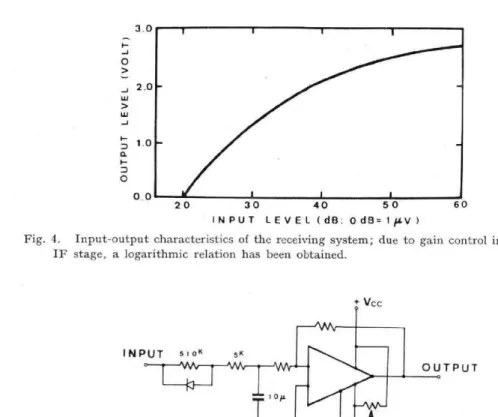
The output signal from the pre-amplifier has the intensity, 2x 10⁻⁴ Volt for the threshold. This provides sufficient level for the usage of FET, for the first stage of IF, with the input impedance of 500 kS2. The second IF stage has feed back loops for the automatic control of the gain; this approximately gives the logarithmic function
140 H. OYA, A. MORIOKA and M. KONDO 3.0 0 2.0 11.1 11J -J 1 . 0 0. D O 0.0 20 30 40 50
INPUT LEVEL (dB; 0 dEi-, 1 auv Fig. 4. Input-output characteristics of the receiving system; due to gain
IF stage, a logarithmic relation has been obtained.
6 0
control in the second
INPUT WINN TIT Vcc OUTPUT - Vcc
Fig. 5. Minimum reading circuit; the time constant for increasing signals is selected to be 100 times longer than that for decreasing signals to obtain steady recording for the white noise.
as has been given in Fig. 4. The detected quasi DC signal is recorded by usual pen-recorders that are fed through the minimum reading circuit (see Fig. 5.).
4. Observation
The decameter waves have been received from October 20, 1974. Several examples are given in Fig. 6 to 8. Since the waves were received with broad directional characteristic, for the present case, the galactic decameter wave is one of the dominant objects of this observation as has been given in Fig. 6. The maximum value of this galactic decameter waves is approximately 5dB (0 dB is equal, in this case, to 10-6
Volt) which gives the intensity of 3.78 x 10⁻¹⁹ Watt/m2Hz.
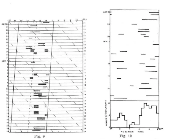
Separated from the general recording trend, that is indicating the galactic decameter waves, a sporadic emissions that approach sometimes to 3 dB out of the galactic emission can be identified. These sporadic emissions are indicated between the arrows in Fig. 6. The different examples of these sporadic emissions for Oct. 27 and Oct. 28 are selected in Fig. 7 and 8. All obtained sporadic type emissions are plotted versus the observed local time in Fig. 9; the diagram is scaled with the Jovian rotation period of 9h 55m 29s that is used as a recurrence period of the Jovian decameter wave emissions in the previous works. In the diagram, the occurence of the decameter
RECEPTION OF THE JUPITER DECAMETER WAVES 141
Fig. 6. Example of the recorded result of the decameter waves from the planet and the galaxy; a monotonic background noise is the decameter wave from the galaxy and sporadic emissions indicated between the arrows are identified coming from Jupiter . This is the case for the observation in Oct. 29, 1974. 19.945 MHz 24.320 MHz OCT. 27 1974 Fig. 7. d
12
1 1 I II2d13
Same as Fig. I „6 for the case observed in Oct. 27, 1974.
19.945 MHz 24.320 MHz OCT. 23 1974 Fig
12
d9
i i12d13
142 H. OYA, A. MORIOKA and M. KONDO OCT. NOV. t, to 8 20 \ I 2 \ 21 1- \ I \ \ I I \ \ I \ \I N\ I \ I \ NI I . I = 1 \
F
I\ T \ 1 I = I \ NI NI \ I I = IN NI N=1 NI \ IN N1 1 \ II \
N I \ I\ I \ 1\ -= = 1 IN ' IN I \ =1 N I IN I • - — -I \ I . . . . Fig. Fig. tahLT 121 27 28 23 30 31 2 3 II 5 8 7 e 10 tt t2 13 15 16 to IB 20 27 22 23 24 OC NOV W U 2 W Y 7 U U O O w m z;; 0" 2 CO TATION 4is TIME COW"
Fig. 9 Fig. 10
9. The occurence of the Jupiter decameter waves versus the local time; the observed data are indicated by thick lines within the visible range of Jupiter. Number of the thick lines in a given section is corresponding to the number of the observed point frequencies.
10. Occurence frequency of the Jupiter decameter waves versus the rotation period of the planet.
wave emissions is separated into two categories. The first is the case where the emission coincides with the predicted phase of the Jupiter rotation; and the second is the case where the emission occurence is shifted from the predicted time for the first category emissions.
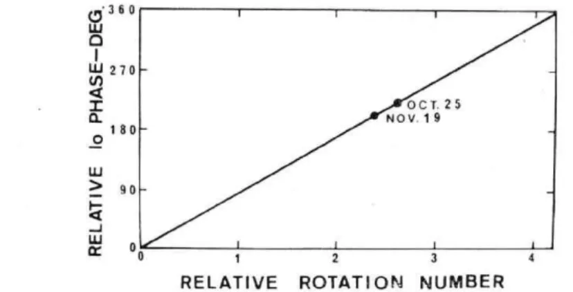
All the data that belong to the first and the second categories are plotted, in Fig. 10, versus the relative Jovian longitude that is rotating with the period, 9h 55m 29s. It is again confirmed that the emissions of the first category are taking place in a given interval of the rotational periods of the planet. The emissions of the second category occure at phases 3 or 4 hour prior to the emissions of the first category. Thus we can conclude that the majority of the emissions (the emissions of the first category) are taking place at the so called main source. The emissions of the second category are generated then at the early source though the ocurrence is less frequent. The emission of this early source seems to be controlled by the position of To as has been reported by Bigg (1964) and by other observation stations. Though the observed results of the early source emissions are limitted in two cases, for the present time, we can plot the emission data with respect to the Jo position as has been given in Fig. 11.
RECEPTION ON THE JUPITER DECAMETER WAVES 143 0'360 LIJ 270'- - U) OCT.25 • NOV.19 180- O La so - La cr 00 1 2 3 4 RELATIVE ROTATION NUMBER
Fig. 11. Occurence of the early source emissions versus the Io position and the rotation phases of the planet; the emissions from early source are limitted only in a given relative
phase of Io satellite as has been given by the cases of Oct. 25 and Nov. 19, 1974.
5. Conclusion
A new station of the Jupiter decameter wave reception has been built at Mt. Zao Observatory, Tohoku University. The system employs the dipole antenna, with a quarter wave length elements, that is equipped with a set of reflector and gives the decameter wave power to the amplifier with input impedance 75Q. The pre-amplifier has the threshold noise level, 2.4 x 10⁻⁸ Volt. The observation has been started at Oct. 20, 1974. The galactic and Jovian decameter waves were identified giving the value 5 x 10-19 Watt/m2Hz for the galactic waves and 2 x 10⁻²' Watt/m2Hz for the Jovian decameter waves. The result of the Jovian decameter waves indicate clear separation of two locations for the emission sources. One is located at the so called main source and the other is lacated at the early source. The emission from the early source indicates the To satellite control with respect to the decameter wave origin that is located in the Jovian plasmasphere.
Acknowledgement: The authors would like to express sincere thanks to Prof. H. Kamiyama and his colleague for their cooperations to develop the observation station.
References
Alexander, J.K., 1967: NASA Rep. No-X-615-67-531.
Bigg, E.K., 1964: Influence of the satellite Io on Jupiter's decametric emission, Nature 203, 1008.
Burke, B.F., and K.L. Franklin, 1955: Radio emission from Jupiter, Nature 175, 1074. Carr, T.D., A.G. Smith, H. Bollhagen, N.F. Six, and N.E. Chatterton, 1961: Recent decameter
wave-length observations of Jupiter, Saturn and Venus, Astrophys. J. 134, 105. Ellis, G.R.A., 1965: The decametric radio emissions of Jupiter, Radio Science 69D, 1513. Oya, H., 1974: Origin of Jovian decameter wave emissions conversion from the electron
cyclotron plasma wave to the ordinary mode electromagnetic wave, Planet Space
Sci. 22, 687.