東北大学機関リポジトリTOUR

(1)

Orbital diamagnetism of graphene

nanostructures

著者

大湊友也

学位授与機関

Tohoku University

(2)

Master Thesis

Orbital diamagnetism of graphene nanostructures

（グラフェンナノ構造体における軌道反磁性）

Yuya Ominato

Department of Physics, Graduate School of Science

Tohoku University

(3)

(4)

Chapter 1 Introduction

Graphene is one-atom-thick crystal which consists of a single sheet of carbon atoms, and the thinnest crystal ever produced. Theoretically, the electronic property of graphene was first studied as a simplified model of three-dimensional graphite, which is a layered ma-terial composed of graphenes. [1, 2, 3, 4] Two-dimensional graphene itself was considered as a purely theoretical material, but after the fabrication of graphene using a mechanical exfoliation,[5] enormous effort has been devoted to understanding its physical properties experimentally and theoretically. [6] Graphene has a characteristic band structure, where the valence and conduction bands stick together with a linear dispersion at corners of Bril-louin zone represented as K and K′. Using an effective-mass approximation, the electronic states of graphene in the vicinity of Fermi level are described by the relativistic Dirac equa-tion with vanishing rest mass. [1, 2, 3, 7, 8, 9, 10] This notable electronic band structure

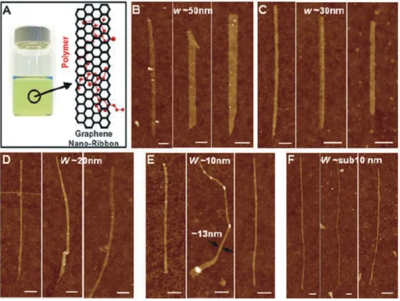
Figure 1.1: Chemically derived graphene nanoribbons with several width. All scale bars indicate 100nm. From [19].

(7)

2 CHAPTER 1. INTRODUCTION

Figure 1.2: STM imaging and spectroscopy on graphene flakes grown by CVD on Ir(111). (a) Large-scale STM image of graphene flakes (G) on an Ir(111) subtrate. Small graphene flakes have been indicated by red circles. (b) STM topography of a small graphene flake with an overlaid atomic model which has perfect hexagonal symmetry with 7 benzene ring along edges. (c) dlnI/dlnVb spectra measured on the points indicated in (b), the green

bars indicate the bias voltages corresponding to the two resonances in the spectra shown in (c). (e) The corresponding LDOS maps calculated for a particle in a box at the indicated energies and the underlying eigenstates. From [22].

gives rise to various unusual physical properties diﬀerent from the conventional electron systems. [10, 11, 12, 13, 14, 15, 16]

Recently, developments in experimental techniques enables to fabricate a various kind of nanostructures such as ribbons and flakes out of graphene. Graphene nanoribbons were first fabricated by top-down approaches using lithographic technique for exfoliated graphene films. [17, 18] Later, with the emergence of bottom-up approaches such as chemical syn-thesis and chemical vapor deposition (CVD), the control of the final system geometry has been significantly improved, and it is now possible to produce graphene systems of differ-ent size and forms with atomically smooth edges, ranging from the quasi-one dimensional ribbons to the zero-dimensional flakes. [19, 20, 21, 22, 23, 24] Figures 1.1 and 1.2 show chemically derived graphene nanoribbons, and CVD-grown graphene flakes, respectively. Alternatively, the graphene ribbons with atomically smooth edges can be fabricated by unzipping carbon nanotubes with chemical oxidative process, as shown in Fig. 1.3. [20, 21]

(8)

3

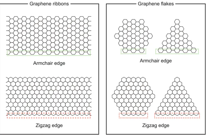
Electronic structures of graphene nanostructures strongly depend on the shapes and the edge configurations. Theoretically, two different edge forms, armchair and zigzag, have been considered as representative forms of interface as shown in Fig. 1.4. It was shown that the zigzag edge is accompanied by zero-energy edge state localized at the boundary, [25] and it is experimentally observed using scanning tunneling spectroscopy (Fig. 1.5). [26] So far, a number of theoretical researches have been devoted to understanding the electronic properties in the graphene ribbon [25, 27, 28, 29, 30, 31, 32, 33, 34] and graphene nanoflakes. [35, 36, 37, 38, 39, 40, 41, 42, 43, 44]

In this thesis, we study the orbital diamagnetism of graphene nanostructures. Gen-erally, the orbital magnetism sensitively depends on the electronic band structure of the system, and sometimes largely deviates from the conventional Landau diamagnetism of free electrons. Particularly, the diamagentism tends to be large in narrow gap systems such as graphite [3, 45, 46] and bismuth [47, 48] due to small eﬀective mass, and becomes even greater in graphene which is a truly zero-gap system. The magnetic susceptibility of bulk graphene contains a singularity expressed as a δ function in Fermi energy εF, which diverges

at Dirac point (εF = 0) where the two bands stick. [3, 49, 50, 51, 52, 53, 54, 55, 56, 57, 58, 59]

The singular magentic behavior is expected to be significantly modified in graphene nanos-tructures due to the quantum confinement effect. The orbital magnetism of finite-sized graphene system was theoretically studied for carbon nanotubes [60, 61, 62] and graphene ribbons [28, 63] while the dependence on the system size and atomic configuraions, nor the

Figure 1.3: (a) Representation of the gradual unzipping of one wall of a carbon nanotube to form a nanoribbon. Oxygenated sites are not shown. (b) The proposed chemical mechanism of nanotube unzipping. From [20].

(9)

4 CHAPTER 1. INTRODUCTION

Armchair edge

Zigzag edge

Graphene ribbons Graphene flakes

Armchair edge

Zigzag edge

Figure 1.4: Geometry of graphene nanostructures.

relation to the bulk limit are not well understood.

Experimentally, the magnetic property of graphene-based materials was investigated for bulk graphite [64, 65, 66], nanographite [67], and exfoliated graphene nanocrystals [68]. There the susceptibility always contains strong diamagnetic background due to the orbital eﬀect, whereas it is also contributed by the spin paramagnetism, [68] and the spin magentic ordering [65, 66, 67, 69] which may be caused by the zero-energy edge states, [28, 43, 44] and atomic defects. In any case, correct understanding of the orbital susceptibility of ﬁnite graphene systems is important to describe the overall magentic property in realistic graphene systems.

In this thesis, we investigate the orbital diamagnetism of graphene ribbons and flakes with various sizes, shapes and edge configurations. For each case we calculate the orbital magnetic susceptibility and the diamagnetic electric current distribution, to find charac-teristic properties peculiar to each different case, and also general tendencies independent of the configuration. For the theoretical model, we use the tight-binding model or the continuum Dirac model depending on the problem. The latter is derived from the tight-binding model using the effective mass approximation, and gives the equivalent result to the original as long as the system size is much larger than the lattice spacing. The virtue of the continuum approach is to enable one to treat the problem analyitically and also to extract the scale-invariant properties originating purely from the nature of the massless Dirac Hamiltonian. We apply the continuum Dirac model to the graphene ribbons, while use the original tight-binding model for graphene flakes where the continuum approach becomes overcomplicated.

The thesis is organized as follows: In Chapter. 2, we introduce the tight-binding model and the eﬀective Dirac model to describe in graphene electrons. In Chapter. 3 and 4, we discuss the orbital diamagnetism of graphene ribbons and graphene ﬂakes, respectively.

(10)

5

Figure 1.5: (a) An atomically resolved UHV STM image of zigzag and armchair edges (9×9nm2_{). (b) Typical dI/dV}

S curve from STS data at a zigzag edge. From [26].

(11)

(12)

Chapter 2 Band model of graphene

In this chaper, we review the band model to describe electrons in graphene which will be used in the following chapters. We first introduce the tight-binding model, and then derive the continuum Dirac model based on it by applying the effective mass approximation. In the last section, we calculate the orbital magnetic susceptibility of bulk graphene using the effective Dirac model, which is shown to be a δ function in the Fermi energy.

2.1 Atomic structure

The Lattice structure of graphene and the ﬁrst Brillouin zone are shown in Fig. 2.1. We have the primitive translation vectors

a = a(1, 0), b = a(−1/2,√3/2), (2.1)

and the vectors connecting nearest neighbor carbon atoms

τ1 = a(0, 1/ √ 3), τ2 = a(−1/2, −1/2 √ 3), τ1 = a(1/2,−1/2 √ 3), (2.2)

where a is the lattice constant given by a≈ 0.246nm. A hexagonal unit cell contains two carbon atoms, which will be denoted by A (black) and B (white). Afterward, we consider boundary conditions for graphene ribbons, so that we deﬁne η as the angle between the x and x′ axes, which is π/6 for the zigzag and 0 for the armchair boundary.

a b y’ x’

τ2

τ3

τ1

B A unit cell ky kx K K’ x y η η (a) (b)

Figure 2.1: (a) Lattice structures and (b) ﬁrst Brillouin zone of graphene.

(13)

8 CHAPTER 2. BAND MODEL OF GRAPHENE

The primitive reciprocal lattice vectors a∗ and b∗ are given by

a∗ = 2π/a(1, 1/√3), b∗ = 2π/a(0, 2/√3). (2.3) The K and K′ points at the corners of the Brillouin zone are given as

K = 2π/a(1/3, 1/√3), K′ = 2π/a(2/3, 0), (2.4) respectively. We have the relations between τ1, τ2, τ3 and K, K′

exp(iK· τ1) = ω, exp(iK· τ2) = ω−1, exp(iK· τ3) = 1, (2.5)

exp(iK′· τ1) = 1, exp(iK′· τ2) = ω−1, exp(iK′· τ3) = ω, (2.6)

where ω = exp(2πi/3).

2.2 Tight-binding model

The motion of graphene electrons can be modelled by the nearest-neighbor tight-binding model of pz orbitals. In a tight-binding model, the wave function is written as

ψ(r) =∑ RA ψA(RA)ϕ(r− RA) + ∑ RB ψB(RB)ϕ(r− RB), (2.7)

where RA= naa + nbb + τ1 and RB= naa + nbb, with integer na and nb, are the positions

of A-sites and B-sites, respectively, and ϕ(r) denotes the wave function of the pz orbital

of a carbon atom located at the origin. Let −γ0 be the transfer integral between

nearest-neighbor carbon atoms and choose the energy origin at that of the carbon pz level. The

parameter γ0 was experimentally estimated in the bulk graphite as γ0 ≈ 3eV.[70, 71] We

substitute this wave function into the Schr¨odinger equation

Hψ(r) = εψ(r), (2.8) multiply it by ψ(r− Rj), (j = A, B), and then integrate it in all space. Then we have

εψA(RA) = −γ0 3 ∑ l=1 ψB(RA− τl), εψB(RB) =−γ0 3 ∑ l=1 ψA(RB+ τl), (2.9)

where the overlap integral between nearest A and B sites is completely neglected for sim-plicity.

Using Bloch’s theorem, we have

ψA(RA)∝ fA(k) exp(ik· RA), (2.10) ψB(RB)∝ fB(k) exp(ik· RB), (2.11) and we derive ( 0 hAB(k) hAB(k)∗ 0 ) ( fA(k) fB(k) ) = ε ( fA(k) fB(k) ) , (2.12)

(14)

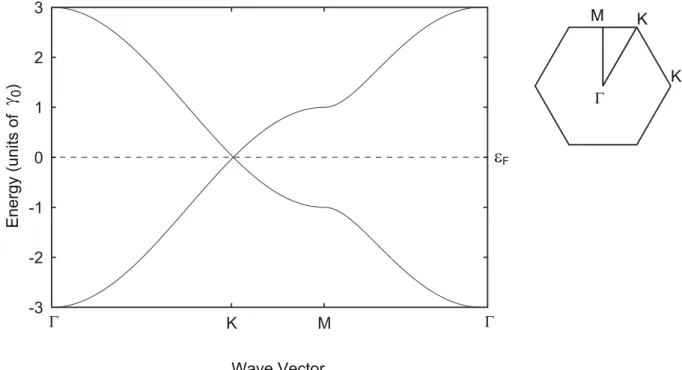
2.3. EFFECTIVE-MASS DESCRIPTION 9 -3 -2 -1 0 1 2 3 Γ K M En e rg y (u n it s o f

γ

)0 Wave Vector Γ

ε

F M _K K` Γ

Figure 2.2: The band structure of graphene obtained in the nearest-neighbor tight-binding model along Γ→ K → M → Γ. The Fermi level lies at the center ε = 0.

with hAB(k) =−γ0 3 ∑ l=1 exp(−ik · τl). (2.13)

The energy bands are given by

ε_±(k) =±|hAB(k)|. (2.14)

The band structure is shown in Fig. 2.2. Using eq. (2.5) and (2.6), it is clear that ε_±(K) =

ε_±(K′) = 0, so that the valence and conduction bands stick together at K and K′ points. Near the K and K′ points, we have

ε_±(K + k) = ε_±(K′+ k) =±~v √ k2 x+ k2y, (2.15) with ~v = √ 3aγ0 2 , (2.16) for |k|a ≪ 1.

2.3 Eﬀective-mass description

In the following, we shall derive an eﬀective-mass (k· p) equation describing states in the vicinity of K and K′points based on the nearest-neighbor tight-binding model. We consider the coordinates (x, y) rotated around the origin by η as well as original (x′, y′) as shown in Fig. 2.1.

(15)

10 CHAPTER 2. BAND MODEL OF GRAPHENE

For a state in the vicinity of zero energy, the wave function can be written as a linear combination of the band states in the vicinity of K and K′ points. There, a small deviation from exact K (K′) point can be included as a slowly-varying envelope function multiplied by Bloch factor eiK·r (eiK′·r). As a result, the wavefuncion is written as

ψA(RA) = eiK·RAFAK(RA) + eiηeiK ′_·RA F_AK′(RA), ψB(RB) = −ωeiηeiK·RBFBK(RB) + eiK ′_·RB F_BK′(RB), (2.17)

in terms of the slowly-varying envelope functions FK

A, FBK, FK

′

A , and FK

′

B . The phase factors

eiη _and −ωeiη _{are attached to simplify the ﬁnal equation. We substitute Eq. (2.17) for}

ψ’s in Eq. (2.9), and derive the diﬀerential equations for the envelop function F , using the

property that it is slowly varying in the atomic scale. We end up with the Schr¨odinger equation for the envelop functions, [2, 3, 7, 8, 9, 10]

H0F (r) = εF (r), (2.18) with H0 =~v      0 ˆkx− iˆky 0 0 ˆ kx+ iˆky 0 0 0 0 0 0 ˆkx+ iˆky 0 0 kˆx− iˆky 0     , (2.19) where ˆk =−i∇, and

F (r) =     FK A(r) F_BK(r) FK′ A (r) FK′ B (r)     . (2.20)

This is relativistic Dirac equation with vanishing rest mass known as Weyl’s equation for a neutrino.

2.4 Orbital diamagnetism of bulk graphene

We derive the orbital magnetic susceptibility for bulk graphene using the Dirac model. In a magnetic ﬁeld B perpendicular to the graphene, Hamiltonian for the K point is written as H = ~ωB ( 0 a a† 0 ) , (2.21) where a = (ℓB/ √ 2)(ˆkx− iˆky),~ωB = √ 2~v/ℓB, ℓB= √

c~/(eB), ˆk = −i∇ + (e/c~)A, and

A(r) is the vector potential giving the magnetic ﬁeld by B =∇ × A. We have [a, a†] = 1. We shall deﬁne a function hn(x, y) such that

hn(x, y) = (a†)n √ n h0(x, y), (2.22) with ah0(x, y) = 0. (2.23)

(16)

2.4. ORBITAL DIAMAGNETISM OF BULK GRAPHENE 11 Then, we have a†hn= √ n + 1hn+1, (2.24) ahn+1= √ n + 1hn, (2.25) a†ahn= nhn. (2.26)

The energy of n-th Landau level is then given by

εn= sgn(n)~ωB

√

|n|, (2.27)

and the wave function by

F_nK= ( sgn(n)h_|n|−1 h_|n| ) , (2.28)

where n = 0,±1, ±2, · · · and sgn(n) is n/|n| for n ̸= 0, and 0 for n = 0. Each Landau level has degeneracy g = 1/(2πℓB) per unit area. Similar expressions can be derived for the K′

point.

The magnetization M is given by the derivative of thermodynamic function Ω

M =− ( ∂Ω ∂B ) µ,T , (2.29)

where µ is the chemical potential and T is the temperature. Since the magnetization is written as M = χB in a weak magnetic ﬁeld, the susceptibility χ is obtained by calculating Ω up to the order of B2, and using

∆Ω =−1 2χB

2_. _(2.30)

For graphene, the thermodynamic function is given by

Ω =−kBT gvgsg ∞ ∑ n=−∞ C(|εn|) ln{1 + exp[(µ − εn)/kBT ]}, =−kBT gvgsg ∞ ∑ n=0 C(~ωB √ n) ( 1− 1 2δn0 ) × ln[1 + 2 exp(µ/kBT ) cosh(~ωB √ n/kBT ) + exp(2µ/kBT )], (2.31)

where gv = gs = 2 are the valley and spin degeneracies, respectively, and C(ε) is a cutoﬀ

function given by C(ε) = ε α c εα_{+ ε}α c , (2.32)

with cutoﬀ energy εc and parameter α, (α > 2). Consider a smooth function F (x) and its

integral ∫ _∞ 0 F (x)dx = ∫ h/2 0 F (x)dx + ∞ ∑ j=1 ∫ h/2 −h/2 F (x + hj)dx, (2.33) where h is a small positive number. For suﬃciently small h, we have

h [ 1 2F (0) + ∞ ∑ j=1 F (hj) ] = ∫ _∞ 0 F (x)dx− 1 12h 2 [ F′(0) +1 2F ′₍_∞) ] +· · · . (2.34)

(17)

12 CHAPTER 2. BAND MODEL OF GRAPHENE Let h = (~ωB)2, x = nh, and F (x) = C(√x) ln[1 + 2 exp(µ/kBT ) cosh( √ x/kBT ) + exp(2µ/kBT )]. (2.35) Then, we have Ω =− kBT gvgs 2πℓ2 B(~ωB)2 h ∞ ∑ n=0 C(√x) ( 1−1 2δn0 ) × ln[1 + 2 exp(µ/kBT ) cosh( √ nh/kBT ) + exp(2µ/kBT )], =− kBT gvgs 2πℓ2 B(~ωB)2 ∫ _∞ 0 C(√x) ln[1 + 2 exp(µ/kBT ) cosh( √ nh/kBT ) + exp(2µ/kBT )]dx + kBT gvgs 2πℓ2 B(~ωB)2 h2 12 exp(µ/kBT )/(kBT )2 [1 + exp(µ/kBT )]2 +· · · . (2.36) Note that the derivative of the cutoﬀ function at x = 0 can safely be neglected. Therefore, we have ∆Ω = gvgs e2_v2 12πc2B 2 ∫ _∞ −∞ ( −∂f (ε) ∂ε ) δ(ε)dε, (2.37) where f (ε) = 1/[1 + eβ(ε−µ)] is the Fermi distribution function with the chemical potential

µ. The susceptibility is derived as [3, 49, 50] χDirac(µ; T ) =−gvgs e2_v2 6πc2 ∫ _∞ −∞ ( −∂f (ε) ∂ε ) δ(ε)dε. =−gvgs e2_v2 24πc2 1 kBT cosh2[µ/(2kBT )] . (2.38) In the limit of T → 0, the susceptibility becomes

χDirac(µ) =−gvgs

e2_v2

6πc2δ(µ). (2.39)

Note that this expression is independent of the detail of the cutoff function. Eq. (2.39) indicates that the susceptibility diverges at the Dirac point and vanishes otherwise. This is significantly different from the conventional Landau diamagnetism, in which the sus-ceptibility is simply proportional to the density of states. The calculation of the Landau diamagnetism is briefly presented in Appendix A.

(18)

Chapter 3 Graphene Ribbons

3.1 Formulations

3.1.1 Eﬀective-mass description

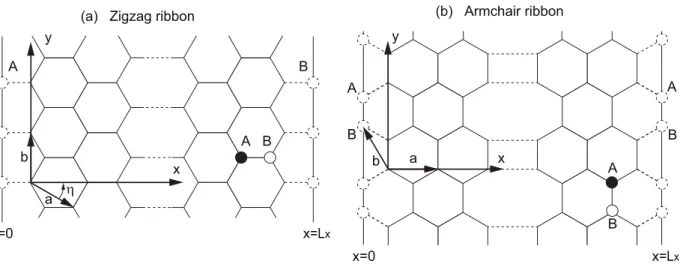
In this chapter, we condiser the zigzag and armchair graphene ribbons, of which atomic structures are illustrated in Fig. 3.1 (a) and (b), respectively. For both cases we set y-axis along the ribbon, and set x = 0 and Lx to the line of missing sites nearest from the edge.

η is the angle between x axis and a, which is π/6 for zigzag, and 0 for armchair boundary.

The electronic states of the graphene ribbon can be correctly described by setting the appropriate boundary condition to the eﬀective-mass Hamiltonian. [31] Now the eigenstates are labeled by ky since the system is translationally symmetric along y-axis. An eigenstate

of Eq. (2.18) with ky and the energy ε is generally written as

F (r) = eikyy     Aeikxx_{+ Be}−ikxx s(Aei(kxx+θ)− Be−i(kxx+θ)) Ceikxx_{+ De}−ikxx s(Cei(kxx−θ)− De−i(kxx−θ))     , (3.1) where k_x2 = ε2/~2v2 − k_y2, eiθ = (kx + iky)/ √ k2

x+ k2y, s = ε/|ε|, and A, B, C and D are

numbers to be determined by satisfying the boundary condition, as we will argue in the following.

(a) Zigzag ribbon (b) Armchair ribbon

x x B A y x=0 x=Lx b a η A B a b y A B A A B B x=0 x=Lx

Figure 3.1: Atomic structures of graphene ribbons with (a) zigzag boundary and (b) arm-chair boundary, respectively. Dashed circles indicate missing sites beyond the boundary.

(19)

14 CHAPTER 3. GRAPHENE RIBBONS

3.1.2 Zigzag boundary

In the zigzag ribbon, the boundary condition is given by ψA(RA) = 0 at x = 0, and

ψB(RB) = 0 at x = Lx. By using Eq.(2.17), this is translated to the condition for the

envelope function as

F_AK(0, y) = 0,

F_BK(Lx, y) = 0,

F_AK′(0, y) = 0,

F_BK′(Lx, y) = 0, (3.2)

which keeps the states at K and those at K′ independent. For an eigenstate for the K point, we apply the ﬁrst two lines of Eq.(3.2) to Eq.(3.1), to obtain

A + B = 0,

s(Aei(kxLx+θ)− Be−i(kxLx+θ))_{= 0.} _(3.3)

To have a solution other than A = B = 0, we require [31]

ky =

kx

tan kxLx

. (3.4)

For given ky, we deﬁne kn(n = 0, 1, 2,· · · ) as solution of Eq.(3.4) in kx satisfying

nπ < knLx < (n + 1)π. Corresponding eigenstates and the energy are obtained as Fsnky(r) = An eikyy √ LxLy     i sin knx s(−1)n+1_{sin k} n(x− Lx) 0 0     , An = ( 1− sin 2knLx 2knLx )_−1/2 , εsnky = s~v √ k2 n+ ky2, (3.5) -5 0 5 10 15 0 tanh kxLx tan kxLx y π/L_x 2π/Lx kx y = kx /ky (kyLx < 1) k1 k0 _κ 0 k1 k2 k2 y = kx/ky (kyLx > 1)

(20)

3.1. FORMULATIONS 15 for n = 0, 1, 2,· · · . For the normalization of the wavefunction, we assumed the periodic boundary condition in y-direction with a large enough period Ly.

Solution kn is obtained by searching for crossing points of tan kxLx and kx/ky as

illus-trated in Fig. 3.2. When kyLx > 1, the ﬁrst solution k0 becomes a pure imaginary number

iκ0 which satisﬁes

ky =

κ0

tanh κ0Lx

. (3.6)

The wavefunction and the energy then becomes

Fs0ky(r) = A0 eikyy √ LxLy     i sinh κ0x −s sinh κ0(x− Lx) 0 0     , A0 = ( −1 + sinh 2κ0Lx 2κ0Lx )_−1/2 , εs0ky = s~v √ −κ2 0+ ky2. (3.7)

This actually describes the edge state localized at the boundary x = 0 and Lx giving a

nearly ﬂat energy band. [25, 27, 28]

The eigenenergy εsnky represents the n-th branch of conduction (s = +) and valence

(s = −) bands respectively. Energy band structure of K as a function of ky is shown as

solid curves in Fig. 3.3(a). Eigenstates for K′point are obtained similarly, where the energy band structure is equivalent to Fig. 3.3(a) with ky inverted to −ky. The ﬂat band of edge

states of K and K′ are connected in a wave number away from K or K′. [25, 27, 28]

3.1.3 Armchair boundary

In the armchair ribbon, the boundary condition imposes both of ψA(RA) = 0 and ψB(RB) =

0 at each of x = 0 and x = Lx. The corresponding conditions for the envelope functions

are written as F_AK(0, y) + F_AK′(0, y) = 0, F_BK(0, y)− F_BK′(0, y) = 0, F_AK(Lx, y) + ω−2NFK ′ A (Lx, y) = 0, F_BK(Lx, y)− ω−2NFK ′ B (Lx, y) = 0, (3.8)

where N = Lx/a is the number of honeycomb lattices between x = 0 and Lx, which can

be integer or half-integer depending on the position of the edge. Applying above conditions to Eq.(3.1), we obtain

   

1 1 1 1

eiθ −e−iθ −e−iθ eiθ eiλ _e−iλ _αeiλ _αe−iλ

ei(λ+θ) _−e−i(λ+θ) _−αei(λ+θ) _αe−i(λ+θ)

        A B C D     =     0 0 0 0     , (3.9) where α = ω−2N and λ = kxLx. The determinant of matrix in Eq.(3.9) should vanish to

have a non-zero solution. This condition is reduced to

kx = kn≡ π Lx ( n−ν 3 ) , n = 0,±1, ±2, · · · , (3.10)

(21)

16 CHAPTER 3. GRAPHENE RIBBONS ν is an integer (0,±1) deﬁned by

2N = 3m + ν, (3.11)

with integer m. The eigenstate and energy are obtained as

Fsnky(r) = eikyy 2√LxLy     eiknx sei(knx+θ) −e−iknx se−i(knx−θ)     , εsnky = s~v √ k2 n+ ky2. (3.12)

When ν = 0, the energy bands of n = 0 and s = ± stick together and thus the system is metallic, while otherwise a gap opens at zero energy and the system becomes a semiconductor. Energy bands for metallic armchair ribbon (ν = 0) and semiconducting armchair ribbon (ν =±1) are shown in Fig. 3.3(b) and (c), respectively. In (c), the labeling

n is for the case of ν = +1, while n becomes −n in ν = −1.

3.1.4 Orbital susceptibility

To calculate the orbital diamagnetism, we consider a graphene ribbon under a uniform magnetic ﬁeld B perpendicular to graphene plane. We take the Landau gauge and set the vector potential as A(r) = [ 0, B ( x− Lx 2 )] . (3.13)

The Hamiltonian in presence of the magnetic ﬁeld is obtained by replacing ˆk by ˆk+eA/(~c),

as

H = H0+ δH, δH =

e

cvˆyAy, (3.14)

where c is the light velocity, and

ˆ vy = 1 ~ ∂H ∂ˆky = v     0 −i 0 0 i 0 0 0 0 0 0 i 0 0 −i 0     . (3.15)

The operator of the electric current density is given by

ˆ jy(r) =− e 2{ˆvyδ(r− r ′_{) + δ(r}_{− r}′_)ˆ_v y} . (3.16)

In the ﬁrst order perturbation in δH, the expectation value of the current density is written as jy(r) = ∑ α f (εα) ∑ β(̸=α) 2Re [ (δH)αβ(ˆjy(r))βα ] εα− εβ , (3.17) where α and β represent the unperturbed eigenstates of graphene ribbon, and f (ε) is the Fermi distribution function.

(22)

3.2. NUMERICAL RESULTS 17 In a zigzag ribbon, the current density always vanishes at the edges x = 0 and Lx, while

it is not generally the case in armchair ribbons. This is obvious from at the matrix element of ˆjy between two eigen states F and F′,

⟨F′_|ˆj y(r)|F ⟩ = iev [ F′KA(r)∗FBK(r)− F′KB(r)∗FAK(r) ] . (3.18) In the wavefunction of zigzag ribbon, Eqs. (3.5) and (3.7), the component F_AK is zero at

x = 0, and F_BK is at Lx, so that Eq. (3.18) vanishes at the both edges.

The current density on xy-plane is related to the local magnetic moment m(r) in z-direction by jx = c ∂m ∂y, jy =−c ∂m ∂x. (3.19)

In the present case, m(r) depends only on x so that the total magnetization per area is

M = 1 LxLy ∫ Lx 0 ∫ Ly 0 m(x)dxdy = 1 cLx ∫ Lx 0 ( x− Lx 2 ) jy(x)dx. (3.20)

The magnetic susceptibility is written as

χ = lim B→0 M B = 2 cLxLy ∑ α f (εα) ∑ β(̸=α) (δ_H/B)_αβ2 εβ − εα . (3.21) We calculate Eqs. (3.17) and (3.21) numerically. As we have inﬁnite energy bands below zero, we introduce a cut-oﬀ function C(εα) which smoothly vanishes |εα| > εc. In

the following, we take εc = 50ε0 where

ε0 =

2π~v

Lx

(3.22)

is the typical energy scale for the subband structure. The result is actually converging in the limit of large εc.

In the graphene ribbon, the characteristic unit of the susceptibility can be chosen as

χ0 = gvgs e2v2 6πc2 1 ε0 . (3.23)

3.2 Numerical Results

3.2.1 Magnetic susceptibility

Lower panels of Fig.3.3 show the orbital susceptibility χ(εF) of (a) zigzag, (b) metallic

armchair (ν = 0) and (c) semiconducting armchair (ν =±1) ribbons at zero temperature, where the upward direction represents the negative (i.e., diamagnetic) susceptibility. The ﬁgures are to be compared with the band structures in upper panels. In every case, the magnitude of χ becomes the maximum at εF = 0, and oscillates as a function of εF in

accordance with the subband structure. In the positive energy region, for example, the curve sharply rises when a subband starts to be occupied by electrons, while it tends

(23)

18 CHAPTER 3. GRAPHENE RIBBONS ε_F (units of ε0) -χ (u n it s o f χ 0 ) k y (u n it s o f 2 p /Lx )

(a) Zigzag ribbon (b) Armchair ribbon (ν=0) (c) Armchair ribbon (ν= 1)

0 0 0 2 -2 1 -1 1 -1 2 ε_F (units of ε0) εF (units of ε0) 0 1 -1 -1 0 1 n=0 1 2 n=0 s=+ s=− n=0 1 -1 -2 2 s=+ s=− s=− s=+ 0 1 2 +_-2 +_-1 0 0 1 -1 -2 2 1 + - +-2 +

-Figure 3.3: Band structure (upper panel) and magnetic susceptibility as a function of

εF (lower), of (a) zigzag, (b) metallic armchair (ν = 0) and (c) semiconducting armchair

(ν =±1) graphene ribbons. In upper panels, solid (black) and dashed (red) curves indicate the band structures at zero and a finite magnetic field, respectively. For the latter, the energy band is calculated with the perturbation theory in a magnetic field B. where we take

B = B0 for (a), and B = 0.5B0 in (b) and (c) for illustrative purpose, and B0 = (ch/e)/L2x.

-χ

(u n it s o f

χ

0 ) 0 1 -1 2

µ

(units of

ε

0) 0 -4 -2 2 4 k_BT/ε0=0 0.80 0.16 Armchair ribbon (ν=0)

Figure 3.4: Magnetic susceptibility against chemical potential µ for metallic armchair rib-bon (ν = 0) at several diﬀerent temperatures.

(24)

3.2. NUMERICAL RESULTS 19 x coordinate (units of L_x) 0 0.2 0.4 0.6 0.8 1.0 -20 -10 0 10 20 Zigzag ribbon Armchair ribbon (ν=0) Armchair ribbon (ν= 1)+₋ C u rre n t d e n si ty (u n it is o f c χ0 B / Lx )

Figure 3.5: Diamagnetic current density jy(x) of diﬀerent types of graphene ribbons with

εF = 0 at T = 0.

to decrease otherwise. In large |εF|, the amplitude of the oscillation slowly attenuates

approximately in proportional to 1/√|εF|.

The oscillating feature can be understood in terms of the band energy shift in an infinitesimal magnetic field. In the upper figures of Fig. 3.3, we plot as broken curves the energy band in some small B calculated by the second order perturbation. Here the amplitude B is set to some finite value for illustrative purpose. Generally the system is diamagnetic when the total energy shift caused by B is positive, and paramagnetic when negative. In the metallic armchair ribbon (b), for example, we see that a pair of the first subbands (n = 0, s =±) shift towards zero energy, due to the level repulsions from excited subbands nearby. All other bands (|n| ≥ 1) move in the opposite direction away from zero energy, while the absolute shifts are much smaller than that of n = 0.

When εF is zero, the energy gain of the ﬁrst valence band (s = −, n = 0) exceeds the

energy loss of all other valence bands (s =−, |n| ≥ 1), resulting in the total diamagnetism. When εF is shifted to positive side, the diamagnetism decreases because the ﬁrst conduction

band (s = +, n = 0) has a negative shift and gives paramagnetism. When the second conduction band (s = +,|n| = 1) starts to be ﬁlled, the susceptibility suddenly jumps to diamagnetic direction, because the shift is positive there and also the density of states diverges at the band bottom. The oscillation of other types, (a) and (c), can be explained in a similar manner.

In Fig. 3.4, the susceptibility at several diﬀerent temperatures is plotted as a function of the chemical potential µ. We here choose the metallic armchair ribbon (ν = 0) while the qualitative property is the same in other cases. We see that the oscillation rapidly disap-pears once kBT becomes of the order of ε0, i.e., the thermal broadening energy is as large as

the subband interval energy, and we are left with only a single diamagnetic peak at εF = 0.

When kBT >∼ε0, the curve becomes almost identical with the bulk susceptibility, Eq. (2.38),

or the thermally-broadened delta function. When we ﬁx the temperature and increase the ribbon width instead, we would see that the oscillatory curve of χ(µ) is shrinking in the horizontal direction as the energy scale ε0 decreases, and, once ε0 becomes as small as kBT ,

the oscillation vanishes and the curve goes to the bulk limit. Similar behavior is observed in all the types of ribbons considered here, and the ﬁnite size eﬀect always disappears when

(25)

20 CHAPTER 3. GRAPHENE RIBBONS Armchair ribbon (ν=0) 0.2 0.4 0.6 0.8 1.0 -2 -1 0 1 2 x coordinate (units of Lx) εF (u n it s o f ε0 ) 20 0 -20 0 j y (u n it s of c χ0 B / L x )

Figure 3.6: Two-dimensional density plot jy(x; εF) of the diamagnetic current density of

metallic armchair ribbon (ν = 0), as a function of position x (horizontal axis) and Fermi energy (vertical). hv/(2πk_BT) k_BT/_ε₀=0 0.80 0.16 -20 0 -10 10 20 C u rre n t d e n si ty (u n it is o f c χ0 B / Lx ) x coordinate (units of L_x) 0 0.2 0.4 0.6 0.8 1.0 Armchair ribbon (ν=0)

Figure 3.7: Diamagnetic current density jy(x) of metallic armchair ribbon (ν = 0) with

εF = 0, at several diﬀerent temperatures. The vertical arrows indicate the characteristic

(26)

3.2. NUMERICAL RESULTS 21

3.2.2 Diamagnetic current density

Fig. 3.5 shows the diamagnetic current density jy(x) in diﬀerent types of graphene ribbons

at εF = 0 and T = 0, calculated in the ﬁrst order perturbation of B. The unit of current

density is taken as cχ0B/Lx. The current ﬂows in opposite directions in the left-hand side

and right-hand side of the ribbon, to make a magnetization perpendicular to the layer. Reﬂecting the absence of the characteristic length scale, the current distribution is not localized to the edge but spread in the entire width in a form of slowly-varying monotonic function.

In zigzag ribbons, the current density actually becomes absolute zero at x = 0 and

Lx, in accordance with the constraint argued in the previous section. The current sharply

drops to zero at the edges, and some oscillatory feature remains around the edge due to a finite cut-off energy. When we increase the energy cut-off (not shown), the curve appears to slowly approach a fixed curve having a discontinuous jump at the edges. In the armchair ribbons, jy is not necessarily zero but logarithmically diverges at the both edges. The

numerical calculation converges much more rapidly there, since there is no discontinuity as in the zigzag case.

Fig. 3.6 is the two-dimensional density plot jy(x; εF) of the diamagnetic current density

of metallic armchair ribbon, as a function of position x (horizontal axis) and Fermi energy (vertical). In increasing εF, the current distribution begins to oscillate as a function of x,

with a characteristic wave number of the order of kF = εF/(~v).

The temperature dependence of the current density at µ = 0 is shown in Fig.3.7 for the same metallic armchair ribbon. When kBT becomes as large as ε0, the current distribution

is localized at the boundary forming the counter edge currents. This is the same tempera-ture range where the oscillation of χ disappears and the bulk limit is achieved. The depth of the current distribution is characterized by

λedge(T ) =

~v 2πkBT

, (3.24)

which shrinks in increasing temperature. With the band velocity of graphene, v ≈ 106

m/s, it is estimated as λedge ≈ [1/T (K)]µm.

This behavior is intuitively explained using the plot of jy(x; εF) in Fig.3.6. The current

density at a ﬁnite T is obtained by integrating jy(x; εF) in εF with the thermal averaging

factor −∂f/∂ε. The current of the middle part of the ribbon vanishes in averaging the oscillating function in εF, while the cancellation is not complete only near the edges, since jy

is always positive and negative in left and right ends, respectively. The similar temperature dependence of the current distribution is found in other types of ribbons considered here. This suggests that, in any finite pieces of graphene with length scale L, the finite-size effect disappears when kBT >∼ε0, and then the diamagnetic current circulates only near edge with

a depth λedge. This is actually conﬁrmed for graphene ﬂakes in Chapter. 3.

The diamagnetic current distribution in graphene is signiﬁcantly diﬀerent from conven-tional electron system. In Appendix B, we calculate the current distribution in a ribbon of usual two-dimensional electron gas, where we will see that the diamagnetic current is always localized near the edge with a depth of the Fermi wavelength, as long as the Fermi energy is much larger than kBT .

3.2.3 Relation to spin paramagnetism

We neglect the eﬀect of the electron spin through out the present analysis. In a zigzag ribbon, particularly, the large density of states contributed by the zero-energy ﬂat band is

(27)

expected to give a signiﬁcant magnitude of Pauli paramagnetism and reduce the orbital diamagnetism. [28]

The ratio between two eﬀects can be quantitatively estimated as follows. The suscep-tibility of Pauli paramagnetism is given by

χpara =

(_g 2

)

µ2_BD(ε), (3.25) where g ∼ 2 is the g-factor for graphene electron, µB = e~/(2mc) is the Bohr-magneton

with m being the free-electron mass, and D(ε) is the density of states per area given by the zero-energy ﬂat band. Since the number of edge states accommodated in a ribbon of the length L is∼ L/a per spin and per valley, [28] we have

D(ε)∼ gvgs L2

L

aδ(ε), (3.26)

which gives a delta-function singularity in χpara.

By comparing χpara with the bulk orbital diamagnetism χDirac, Eq. (2.38), we obtain

χpara χDirac = 3π 2 ~2 m2_v2_aL ∼ 1.0 × a L, (3.27)

which is negligible in a wide strip with L ≫ a. In a low temperature such that kBT <∼ε0,

however, χDirac cannot be regarded as thermally broadened delta-function due to the eﬀect

of the subband formation, and then χpara overcomes χDirac only at εF = 0.

3.3 Carbon Nanotubes

The carbon nanotube is a quasi-one-dimensional system similar to graphene ribbon, but diﬀerent in that there are no edges. [72, 73] Experimentally, graphene nanoribbons with smooth edges can be obtained by unzipping the carbon nanotubes, i.e., lengthwise cutting of carbon nanotube side walls. [20, 21] Then we may ask which of the ribbon and the original nanotube has greater diamagnetism, and how the susceptibility oscillation in εF changes

in unzipping. The orbital susceptibility of carbon nanotube was theoretically studied for small Fermi energies in the eﬀective mass approximation [60, 61]. Here we compute full Fermi energy dependence in parallel fashion to the analysis for ribbons.

A carbon nanotube is characterized by a chiral vector,

L = naa + nbb, (3.28)

where the atom at L on a graphene sheet is rolled up onto the origin in constructing a tube. The boundary condition is given by ψA(RA) = ψA(RA+ L) and ψB(RB) = ψB(RB+ L).

For the eﬀective mass wavefunction, it is written as [9]

FK(r + L) = exp ( −2πi 3 ν ) FK(r), FK′(r + L) = exp ( +2πi 3 ν ) FK′(r). (3.29) Here FK_{= (F}K

A, FBK) etc., and ν is an integer (0,±1) deﬁned by

(28)

3.3. CARBON NANOTUBES 23 with integer m.

For K point, the eigenstates are immediately obtained as

F_snkK _y(r) = e ikyy √ 2LxLy     eiknx sei(knx+θ) 0 0     , εsnky = s~v √ k2 y+ kn2, (3.31) where kn ≡ 2π Lx ( n− ν 3 ) , n = 0,±1, ±2, · · · , (3.32) and Lx =|L| and Ly is length of the carbon nanotube. The system is metallic when ν = 0,

and semiconducting when ν =±1. The band structure looks similar to armchair graphene ribbon’s, but the unit of momentum quantization doubled compared to Eq. (3.10), leading to wider energy spacing between subbands. The energy band for K′is obtained by replacing

ky by −ky and also ν by −ν.

When a uniform magnetic ﬁeld B is applied perpendicularly to the nanotube axis, the vector potential can be taken as

A(r) = ( 0, BLx 2π sin 2πx Lx ) . (3.33)

We should note that the expression diﬀers from that for ribbon, Eq. (3.13), because the magnetic ﬁeld perpendicular to the tube surface is not a constant, but a sinusoidal function in x. Except for that, the magnetic susceptibility χtube(εF) is calculated in the same

formula, Eq. (3.21).

The susceptibility of the carbon nanotube is naturally related to that of graphene against a spatial varying magnetic ﬁeld B(q) sin qx with q = 2π/Lx ≡ q0. When we deﬁne

the q-dependent susceptibility of graphene as χDirac(q) ≡ m(q)/B(q), [57] we obtain a

relation

⟨χtube(εF)⟩φ =

1

2χDirac(q0; εF). (3.34) Here⟨ ⟩φ represents an average over a phase factor φ which twists the boundary condition

of carbon nanotube as ψ(r + L) = exp(2πiφ)ψ(r). Physically, the phase factor corresponds to threading a magnetic ﬂux of (ch/e)φ into the nanotube cross section.[9, 60] It changes momentum quantization of Eq. (3.32) to kn = (2π/Lx)(n + φ−ν/3), and the ﬂux averaging

over φ smears the diﬀerence in ν. The factor 1/2 in Eq. (3.34) enters because the average of the squared magnetic ﬁeld on the nanotube surface is B(q0)2/2.

At the zero temperature, χDirac(q; εF) is explicitly evaluated as [57]

χDirac(q; εF) = − gvgse2v 16~c2 1 q θ(q− 2kF) × [ 1 + 2 π 2kF q √ 1− (_2k F q )2 − 2 πsin −1 2kF q ] , (3.35) where kF = |εF|/(~v) is the Fermi wave number and θ(x) is deﬁned by θ(x) = 1 (x > 0)

(29)

-χ

(u n it s o f χ0 ) 0 0.4 -0.4

-χ

(u n it s o f χ0 ) 0 1 -1 εF (units of ε0) 0 1 -1 -2 2 Zigzag ribbon CNT (av.) (a) (b) CNT (ν=0) CNT (ν= 1)+− CNT(ν=0)

Figure 3.8: (a) Magnetic susceptibility of carbon nanotubes. Solid (black), dashed (red) and dotted (green) curves are for metallic (ν = 0), semiconducting (ν =±1), and the ﬂux average, respectively. (b) Magnetic susceptibility of the carbon nanotube of ν = 0 (solid black) and the zigzag ribbon unzipped from the same nanotube (dashed red).

shown to be ⟨∫ ∞ −∞ χtube(εF)dεF ⟩ φ = 1 2 ( −gvgs e2_v2 6πc2 ) , (3.36)

which is exactly half of graphene’s, suggesting that the susceptibility is eﬀectively smaller in nanotube than in ribbon. This is simply because the B-ﬁeld component penetrating the lattice plane is smaller in the nanotube due to its cylindrical shape.

The susceptibility before taking ﬂux average can be calculated in numerics. Fig. 3.8 (a) shows χtube(εF) for the metallic (ν = 0) and the semiconducting (ν = ±1) nanotubes,

together with the ﬂux average. It has an oscillatory behavior similar to the graphene ribbon’s, while χ in |εF| > ~vq/2 completely vanishes after ﬂux average.[57] In increasing

temperature (not shown), the oscillation immediately disappears, leaving a single peak regardless of ν, similar to the graphene ribbon.

Fig. 3.8 (b) compares the susceptibility of a carbon nanotube and that of corresponding graphene ribbon unzipped from the same nanotube. Here we chose a zigzag ribbon as an example, when the corresponding nanotube becomes an armchair nanotube which is always metallic (ν = 0). [9] The oscillation period of the nanotube is approximately twice as large as that of the ribbon, reﬂecting the wider subband spacing. Overall magnitude of χ is smaller in nanotube roughly by factor 2. The integrate of susceptibility in εF diﬀers in

(30)

Chapter 4 Graphene Flakes

4.1 Formulations

In this chapter, we consider four different atomic configurations of graphene flakes as shown in Fig. 4.1, which are characterized by hexagonal or trigonal global shapes and by armchair or zigzag edge termination. For each case, we range the system size from a few nm to a few tens of nm. We describe the motion of graphene electrons using the nearest-neighbor tight-binding model of pz orbitals. The Hamiltonian is written as

H =−γ0

∑

⟨n,m⟩

ei2πϕnm_c†

ncm, (4.1)

where c†_n is the creation operator of π electron at the site n, and ⟨n, m⟩ represents sum-mation over all nearest-neighbor sites. The system is under a uniform magnetic ﬁeld B

(a) (b)

(c) (d)

Hexagonal Armchair Trigonal Armchair

Hexagonal Zigzag Trigonal Zigzag

Figure 4.1: Atomic structures of graphene ﬂakes with (a) hexagonal armchair, (b) trigonal armchair, (c) hexagonal zigzag, and (d) trigonal zigzag ﬂake.

(31)

26 CHAPTER 4. GRAPHENE FLAKES

perpendicular to the graphene plane, which is incorporated by the Peierls phase ϕnm,

ϕnm = e ch ∫ m n dℓ· A, (4.2)

where A(r) is the vector potential giving the magnetic ﬁeld by B =∇ × A.

For each single graphene ﬂake, we diagonalize Hamiltonian Eq. (4.1) and obtain a set of eigenenergies εi. The thermodynamical potential at temperature T and chemical potential

µ is written as

Ω =−kBT

∑

i

ln{1 + exp[(µ − εi)/kBT ]} . (4.3)

The magnetic susceptibility is given by

χ =−1 S ( ∂2_Ω ∂B2 ) µ,T B=0 , (4.4)

where S is an area of the system. To calculate this, we derive the eigenenergies at zero magnetic field and those at a small finite magnetic field, and numerically compute the derivative of the thermodynamic potential. The amplitude of the small field must be chosen so that the level shift from the zero field is smaller than kBT .

The electric current from site m to n is calculated by an operator,

Jnm =−i eγ0 ~ ( ei2πϕnm_c† ncm− h.c. ) . (4.5)

We obtain the expectation value of Jmn for each bond using the eigenstates at a suﬃciently

weak magnetic ﬁeld, where the current amplitude behaves linearly to B.

4.2 Magnetic susceptibility

Fig. 4.2 shows the susceptibility against the chemical potential for four types of the graphene flakes with several different temperatures. The areas of the flakes are taken to be nearly equal to S ≈ (23.5nm)2_{, which includes 1.1}× 104 _{of hexiagonal unit cells. The horizontal}

and vertical axes are scaled by

ε0 = ~v √ S, (4.6) χ0 = gvgse2v2 6πc2_ε 0 , (4.7)

respectively. ε0 represents the energy scale in the Dirac cone associated with the length

scale √S. We also calculated the same quantity for diﬀerent system sizes (not shown) and

found that for each of four types, the susceptibility and the level structure plotted in this scale becomes almost universal as long as √S ≫ a. This is naturally expected from the

fact that the low-energy physics are well described by the Dirac Hamiltonian.

Upper ﬁgure in each panel presents the energy level structure at B = 0, where dashed (black) lines are non-degenerate levels, and solid (red) lines are two-fold degenerate levels. In the low temperature regime, kBT ≪ ε0, we observe that the susceptibility abruptly

changes at every single energy level, and in particular, it exhibits sharp spikes toward the paramagnetic direction (downward in the ﬁgure) at two-fold degenerate levels. This is because the degenerate states, having opposite magnetic moments, split linearly in magnetic

(32)

4.2. MAGNETIC SUSCEPTIBILITY 27 ﬁeld just like spin Zeeman splitting, and this induces paramagnetism in an analogous way to spin Pauli paramagnetism. The contribution to the orbital suscpetibility (per area) from the degenerate states at E0 is written as

χ = 2 Sm

2

δ(µ− E0), (4.8)

where ±m is the magnetic moments of the doublet.

The major difference between armchair flakes and zigzag flakes comes from the zero-energy edge states peculiar to the zigzag edge. [35, 43] In the triangular zigzag flake, Fig. 4.2 (d), there are a number of energy levels exactly at zero energy, of which wavefunctions are shown to be localized at the edge and the degeneracy is as many as the number of edge sites of the system.[35] However, the susceptibility at T = 0 is completely flat there, meaning that the edge states have absolutely no contribution to the orbital magnetism. This is because the edge states are locked to zero energy even in the presence of magnetic field, and do not participate in total energy change.

In the hexiagonal zigzag flake, Fig. 4.2(c), on the other hand, the edge levels slightly shift from zero energy, because in the hexagonal case the edge states of neighboring sides are localized to different sublattices, and they are directly hybridized by the transfer integral connecting A and B sublattices. The energy shift generally depends on the magnetic field, giving some small contributions to the orbital suceptibility as actually observed in Fig. 4.2(c). Nevertheless, the edgestates do not play a significant role in the overall behavior of the orbital magnetism.

As the temperature increases, the spikes and steps in the suscpetibility are smeared out into an oscillatory curve, and in kBT /ε0 & 1, the oscillation eventually disappears leaving

a single diamagnetic peak centered at the Dirac point. In this temperature regime, the finite-size effect is already smeared out and the plot is almost independent of the atomic configuration of the graphene flake. The central diamagentic peak in high T corresponds to the thermally-broadened delta-function in the bulk limit, Eq. (2.38).

In Fig. 4.3, we present an extended plot of the susceptibility curve of kBT /ε0 = 2.22 in

Fig. 4.2, over the whole band region. The energy axis is now scaled by absolute unit γ0,

and the temperature amounts to kBT /γ0 = 0.02 in this unit. The curve is characterized

by the diamagentic peak at the Dirac point, and relatively smaller structures coming from the electronic states outside the Dirac cone (|µ| < γ0). Speciﬁcally, we see tiny Landau

diamagnetism in the quadratic band bottom at µ = ±3γ0, and paramagnetism around

the van Hove singularity at µ = ±γ0. [49, 58, 59] The contribution from the lower-half

spectrum adds up to a paramagnetic oﬀset to the central diamagnetic peak. Namely, the susceptibility near µ = 0 is approximately written as

χ(µ; T )≈ χDirac(µ; T ) + χpara, (4.9) where χpara ≈ 0.37 × gvgse2v2 6πc2_γ 0 . (4.10)

The oﬀset χpara is actually negligible compared to the height of the central peak which is

the order of gvgse2v2/(24πc2kBT ), since kBT is usually much smaller than γ0.

To make the size dependence clearer, we plot in Fig. 4.4(a) and (b) χ(µ = 0; T ) of hexag-onal armchair flakes with several different sizes. The panels (a) and (b) present the same information in different fashions: (a) plots χ in the absolute units γ0 and gvgse2v2/(6πc2γ0)

(33)

(a) Hexagonal Armchair (b) Trigonal Armchair

(c) Hexagonal Zigzag (d) Trigonal Zigzag

µ (units of ε0) − χ (u n it s o f χ0 ) -10 -5 0 5 10 -0.2 -0.1 0.0 0.1 0.2 0.3 0.4 -10 -5 0 5 10 -0.2 -0.1 0.0 0.1 0.2 0.3 0.4 -10 -5 0 5 10 -0.2 -0.1 0.0 0.1 0.2 -10 -5 0 5 10 -0.2 -0.1 0.0 0.1 0.2 kBT/ε0= 0.01 1.11 0.33 2.22

Edge States _{Edge states (144 levels)}

− χ (u n it s o f χ0 ) µ (units of ε0) µ (units of ε0) µ (units of ε0) S = 23.5 [nm]

Figure 4.2: Energy level structure (upper panel) and magnetic susceptibility as a function of µ (lower) at several diﬀerent temperatures, of (a) hexagonal armchair, (b) trigonal armchair, (c) hexagonal zigzag, and (d) trigonal zigzag graphene ﬂakes with the size of

S ≈ (23.5nm)2. In the upper panel, dashed (black) lines represent non-degenerate levels, and solid (red) lines two-fold degenerate levels.

(34)

4.3. COMPARISON TO SPIN MAGNETISM 29 -0.2 0 0.2 0 2 4 6 8 10 -3 -2 -1 0 1 2 3 -1.0 -0.5 0 0.5 1.0 1.5 2.0 µ (units of γ0) − χ (u n it s o f gv gs e 2v 2 / 6 π c 2γ 0 ) tri armchair hexa zigzag tri zigzag hexa armchair kBT/ γ0=0.02 (kBT /ε0=2.22) S = 23.5 [nm]

Figure 4.3: Extended plot of the susceptibility curve of kBT /ε0 = 2.22 in Fig. 4.2, over the

whole band region. The energy axis is now scaled by absolute unit γ0, and the temperature

amounts to kBT /γ0 = 0.02 in this unit. Inset shows the detail of the central peak.

from the Dirac cone, with relative units ε0 and χ0 depending on the system size. In (b),

we see that the curve converges to a single universal curve as the size increases, indicat-ing that the physics there is well described by Dirac equation. The susceptibility agrees with the bulk limit χDirac in the high temperature region kBT ≫ ε0, whereas in kBT . ε0

it deviates from χDirac and reaches some ﬁnite maximum value, where the descrete level

structure becomes signiﬁcant.

The universal curve depends on the detail of the flake shape and the edge configuration. In Fig. 4.4(c), we plot χ(µ = 0; T ) for four different types of graphene flakes in a similar fashion to Fig. 4.4(b). The flake sizes are set to S ≈ (23.5nm)2, which is sufficiently large to achieve the universal limit. In low temperatures, the susceptibility tends to be larger in armchair flake than in zigzag flake, and larger in hexagonal flake than trigonal flake. A similar edge dependence is found in graphene ribbons, where armchair ribbons generally exhibit larger diamagnetism than zigzag ribbons. In the high temperature region, on the other hand, all the curves approaches the bulk limit.

4.3 Comparison to spin magnetism

The orbital magentism always competes with the spin magnetism which has been neglected so far. When we include spin Zeeman splitting, a spin-less energy level at E0 is accompanied

by the Pauli paramagnetism

χPauli= 2 S (_g 2 )2 µ2_Bδ(µ− E0), (4.11)

where g∼ 2 is the g factor for a graphene electron, µB = e~/(2m0c) is the Bohr magneton

and m0 is the bare electron mass. This is similar to the orbital contribution Eq. (4.8),

(35)

of m is shown to be of the order of √Sev/c, which is the only magnetic-moment scale in

the massless Dirac system. m is typically much greater than µB, suggesting that the Pauli

paramagentic eﬀect is generally much smaller than the orbital eﬀect. At S = (1nm)2_{, for}

example, √Sev/c is already as large as 20µB. This in contrast to conventional electron

systems where orbital magnetic moment and spin magnetic moment are both of the order of µB. [74]

In a zigzag graphene ﬂake, a bunch of edge states degenerate at zero energy give excep-tionally large Pauli paramagnetism. The contribution is written as

χPauli = Nedge 2 S (_g 2 )2 µ2_Bδ(µ), (4.12) where Nedge(∼ √

S/a) is the number of edge states. In the low-temperature regime such

that kBT ≪ ε0, this is dominant over the orbital eﬀect near zero energy, since the orbital

susceptibility does not diverge at edge states as already shown. In high-temperature regime

kBT ≫ ε0, the delta-function is thermally broadened and it should be compared to the

bulk orbital susceptibility χDirac, Eq. (2.38). The ratio between two opposite components

approximates χPauli χDirac ∼ _g3π_v_g_s (_m~₀_va)2(g₂)2 √a S ∼ 0.4 × a √ S, (4.13)

so that the Pauli paramagnetism is negligible in a large ﬂake with √S ≫ a. This is

corresponding to Eq. (3.27).

It should be noted that graphene ﬂakes may have lattice vacancies and/or adatoms depending on the experimental condition, and the impurity levels at these defects con-tribute to additional Pauli paramagnetism. Moreover, we remark that there are several experimental studies that report ferromagnetic spin ordering in graphene-based materials. [65, 66, 67, 69] The origin of the spontaneous magnetism is still under debate, while it can be in principle caused by the atomic defects, grain boundaries, and highly-degenerate edge states. [28, 43, 44]

4.4 Diamagnetic current distribution

Fig. 4.5 shows the diamagnetic current distribution induced by the magnetic field in the four types of graphene flakes of the size S ≈ (23.5nm)2 _{at several different temperatures.}

To visualize the global current circulation, we illustrate continuous ﬂux lines obtained by smoothing the original discrete current Jmnon each bond, which is shown in the left insets.

Specifically, we find the potential function Ψ which satisfies J = ez× ∇Ψ, and obtain the

equi-potential lines of Ψ. At zero temperature, the flux circulates entirely on the system reflecting the absence of the characteristic wave length in graphene, while it gradually becomes localized near the edge as temperature becomes higher. The current circulation of zigzag and armchair graphene flakes are globally similar, but the flux lines of armchair flakes exhibit some roughness while it is not observed in zigzag flakes. This actually corresponds to the atomic-scale current circulation in the Kekulé pattern seen in the original current map, [28] which is caused by the inter-valley (between K and K′) hybridization peculiar to the armchair edge.

Fig. 4.6 shows the detailed plots of the electric current as a function of position from the boundary to the center, for (a) the zigzag and (b) armchair ﬂake. The position is labeled by the bond index deﬁned in the inset, and A and B (B’) correspond to the edge and the

(36)

4.5. RANDOMLY STACKED MULTILAYER GRAPHENE 31 center of triangle (hexagon), respectively, which are depicted in Fig. 4.6(c). The current distribution is more edge-localized when T becomes higher, and the typical depth of the edge current is characterized by

λedge= ~v

2πkBT

, (4.14)

as is consistent with the result for graphene ribbons. The current distribution in the atomic scale crucially depends on the edge type even in the high temperature regime, but we can show that the integrated edge current approximates cχDiracB independently of the edge

type, as long as the diamagnetic current is well localized near the edge. When comparing hexagonal and triangular ﬂakes of the same edge type, we see that the curves are almost completely equivalent in kBT /ε0 & 2. This suggests that the current distribution in the high

temperature regime does not depend on the global shape any more but is solely determined by the edge conﬁguration.

4.5 Randomly stacked multilayer graphene

The diamagnetism can be made even greater by stacking graphenes in three dimensions. The recent experimental technique realizes a novel kind of graphene multilayer in which successive layers are stacked with random rotating angles. [75, 76, 77] There it is known that the interlayer coupling is signiﬁcantly weakened and the Dirac cone is kept almost intact near zero energy as long as the rotating angle is not too small. [78, 79, 80, 81] The orbital susceptibility of such a system is expected to be much stronger than graphite in which the delta-function peak of χ(εF) is much broadened and shortened by the regular

interlayer coupling. [82, 83]

Here we consider the orbital diamagnetism of a finite-sized piece of random-stacked graphene multilayers. In calculations, we self-consistently include the effect of the counter magnetic field induced by the diamagnetic current itself. This is essential because, as we will show in the following, the counter magnetic field of this system can be of the same order of the external magnetic field, and even nearly perfect screening is possible in low temperatures.

For simplicity, we completely neglect the interlayer coupling and regard the system as a set of independent single layer graphenes. We also assume that each layer has the identical shape with a characteristic length scale L, and that the system is large enough that the thermal broadening energy kBT is much larger than 2π~v/L. According to the

previous discussions, we then expect that the susceptibility of each layer is given by the bulk limit χDirac in Eq. (2.38), and also the depth of the edge current λedge of Eq. (3.24)

can be neglected with respect to the system size L.

Let us consider a situation where a external ﬁeld Bext is applied perpendicularly to

graphene plane of the random stacked multilayer. The total magnetic ﬁeld B penetrating the system is

B = Bext+ ∆B, (4.15)

where ∆B is the counter ﬁeld caused by graphene electrons. The total ﬁeld B induces the magnetism in each layer, M = χDiracBS, with S being the area of the layer. This is related

to the diamagnetic edge current I of each single layer by

I = cM

東北大学機関リポジトリTOUR

Orbital diamagnetism of graphene

nanostructures

著者

大湊 友也

学位授与機関

Tohoku University

Master Thesis

Orbital diamagnetism of graphene nanostructures

（グラフェンナノ構造体における軌道反磁性）

Yuya Ominato

Department of Physics, Graduate School of Science

Tohoku University

Contents

Chapter 1

Introduction

Chapter 2

Band model of graphene

2.1

Atomic structure

τ2

τ3

τ1

2.2

Tight-binding model

γ

ε

2.3

Eﬀective-mass description

2.4

Orbital diamagnetism of bulk graphene

Chapter 3

Graphene Ribbons

3.1

Formulations

3.1.1

Eﬀective-mass description

3.1.2

Zigzag boundary

3.1.3

Armchair boundary

3.1.4

Orbital susceptibility

3.2

Numerical Results

3.2.1

Magnetic susceptibility

-χ

χ

µ

ε

3.2.2

Diamagnetic current density

3.2.3

Relation to spin paramagnetism

3.3

Carbon Nanotubes

-χ

-χ

Chapter 4

Graphene Flakes

4.1

Formulations

4.2

Magnetic susceptibility

4.3

Comparison to spin magnetism

4.4

Diamagnetic current distribution

4.5

Randomly stacked multilayer graphene

大湊友也