Broken C-shaped extinction curve and
near-limit flame behaviors of low Lewis number
counterflow flames under microgravity
著者
Tomoya Okuno, Takaki Akiba, Hisashi Nakamura,
Roman Fursenko, Sergey Minaev, Takuya Tezuka,
Susumu Hasegawa, Masao Kikuchi, Kaoru Maruta
journal or
publication title
Combustion and Flame
volume
194
page range
343-351
year
2018-06-18
URL
http://hdl.handle.net/10097/00128035
1
Broken C-shaped extinction curve and near-limit flame behaviors of low Lewis
number counterflow flames under microgravity
Authors: Tomoya Okuno
1, Takaki Akiba
1, Hisashi Nakamura
1, Roman Fursenko
2,
Sergey Minaev
2, Takuya Tezuka
1, Susumu Hasegawa
1, Masao Kikuchi
3, and
Kaoru Maruta
1,2Affiliations: 1. Institute of Fluid Science, Tohoku University,
2-1-1 Katahira, Aoba-ku, Sendai, Miyagi 980-8577, Japan.
2. Far Eastern Federal University,
8 Suhanova St., Vladivostok, 690950, Russia
3. Japanese Aerospace Exploration Agency,
2-1-1 Sengen, Tsukuba, Ibaraki 305-8505, Japan.
Type of article: full-length
Corresponding author: Tomoya Okuno
TEL: +81-22-217-5296
FAX: +81-22-217-5296
E-mail: [email protected]
2
Abstract
To examine the effect of Lewis number on the extinction boundary, flame regimes, and the formation of sporadic flames, microgravity experiments on counterflow flames for CH4/O2/Kr
(Le ≈ 0.7–0.8) and CH4/O2/Xe (Le ≈ 0.5) mixtures, and three types of computations, which are
one-dimensional computations with a PREMIX-based code using detailed chemistry, and three- and one-dimensional computations with the thermal-diffusion model using an overall one-step reaction were conducted. In the microgravity experiments, planar flames, planar flames with propagating edges, planar flames with receding edges, star-shaped flames, cellular flames, and sporadic flames were identified, and their regions of existence in the equivalence ratio-stretch rate plane were obtained. Sporadic flames were formed for Xe mixtures but not for Kr mixtures in the experiments. Similarly, sporadic flames were formed at Le = 0.50 but not at Le = 0.75 in the three-dimensional computations with the thermal-diffusion model. Also, the flame regime of sporadic flames extended far beyond the extinction boundaries obtained in the one-dimensional computations in both experiments and the three-dimensional computations. Furthermore, a comparison of the sporadic flames and flame balls in the three-dimensional computations showed that sporadic flames are intermediate combustion modes that segue flame balls to propagating flames.
Keywords
Counterflow premixed flames, Flame ball, Radiative extinction, Flammability limit, Microgravity combustion
3
1. Introduction
Studies on the dynamics and the combustion limits of premixed flames are essential fundamentals for the development of clean combustion technologies such as lean-burn engines. However, a complete and comprehensive understanding on the dynamics and the combustion limits of near-limit stretched premixed flames has not yet been achieved for low Lewis numbers, despite extensive efforts of many researchers. The combustion limits of stretched premixed flames have been widely studied using flames in stagnation flow or counterflow fields [1–10]. Experimental investigations on the combustion limits at low stretch rates have been conducted under microgravity [7,9,10], in order to minimize disturbance to the flame caused by natural convection. These studies have been conducted over a range of Lewis numbers, Le, from 0.97 to 1.8, but studies for even lower Lewis numbers are still scarce.
Focusing on this issue, we have previously conducted counterflow experiments under microgravity using CH4/O2/Xe mixtures (Le ≈ 0.5) at stretch rates from 1.1 to 4.4 s-1 [11–13]. We
have also conducted experimental investigations under microgravity with the effect of radiation reabsorption at slightly higher Lewis numbers (Le ≈ 0.75) using CH4/O2/CO2 mixtures [14]. In
these previous studies, we have shown that transitions to ball-like flames from counterflow planar flames occur at extremely low stretch rates [11–14]. Extension of the combustion limit due to the formation of multiple ball-like flames, termed sporadic flames, has also been obtained in the framework of the thermal diffusion model [13]. Sporadic flames are a group of ball-like flames,
4 which are formed when each cap-like segment in a cellular flame breaks up and close upon themselves [15–18]. Similar flames have also been reported to exist in uniform flows[15–21], tubes [22–25], divergent channels [26], and Hele-Shaw cells [27]. However, the difficulty in experimental observation of these flames which are free from the effect of conductive heat loss or disturbance from natural convection has resulted in incomplete studies on these sporadic flames. Namely, the effects of Lewis number on the combustion limits, formation of sporadic flames, and flame regimes under microgravity remain largely uninvestigated. Therefore in this study, we aim to investigate this issue by using Kr or Xe gas as a diluent for methane and oxygen mixture to change the Lewis number.
Another type of flame that can be observed under microgravity is the flame ball. Flame balls are spherical flames without flame propagation which exist in quiescent mixtures at Lewis numbers sufficiently lower than unity. The existence of flame balls were first suggested by Zel’dovich [28] and was later verified by theoretical [29–31], computational [32–35], and experimental [36,37] investigations. A single ball-like flame in the sporadic flame resemble these flame balls in shape and in the conditions that these flames are formed. However, direct comparisons between the sporadic flames and the flame balls have not been conducted yet. Therefore in this study, we have additionally compared the flame structures, characteristic flame sizes, and the combustion limits of flame balls and the sporadic flames obtained with
5 computations in an attempt to clarify the relation between these two flames.
2. Experimental methods
Microgravity experiments were conducted to obtain the combustion limit, near-limit extinction boundary, and flame regimes of counterflow flames for mixtures with different Lewis numbers. Figure 1 shows a schematic of the experimental apparatus.
The microgravity environment was attained by parabolic flights of an airplane (MU-300) operated by Diamond Air Service Incorporation [38], Japan. The duration of microgravity was around 15–20 seconds, and the gravity levels were on the order of ±0.01 G. In the present study, data were removed for consideration when the gravity level exceeded 0.1 G during the microgravity experiments. To conduct the counterflow flame experiments, two opposed cylindrical burners were placed inside a chamber. Here, the burner inner diameter was 30 mm and the burner distance was from 30 to 45 mm. The burner distance was changed depending on the stretch rate to avoid upstream conductive heat loss to the burners from the flames. A detailed description of the experimental apparatus and the experimental procedure can be found in [7].
In the experiments, CH4/O2/Kr or CH4/O2/Xe premixtures were supplied to both burners,
forming a counterflow field. The mole fraction ratio of O2 to the diluents in the mixtures were set
6 Separate mass flow controllers were used to control the flow rates for each gas component of the mixtures. Each mass flow controller was calibrated before and after each flight using a flow meter (Horiba SF-1U) to ensure that no changes in the applied voltage-flow rate conversion factor
occurs due to the acceleration during the flight. The accuracy of the flow meter measurement is
within ± 1.0 % of the reading point. This results in around ± 2.0 % uncertainty in the equivalence
ratio and ± 1.0 % uncertainty in the stretch rate.
After ignition, the equivalence ratio and/or the stretch rate a were gradually changed to obtain extinction. Here, the global stretch rate was defined as a = 2U/L where U is the mean velocity at the burner outlet and L is the burner distance. In most cases, the stretch rate was kept constant and the equivalence ratio, , was gradually decreased by 0.015 per second. For flame observation, two HD cameras and a high-speed camera equipped with an image intensifier (Photron FASTCAM MC2.1) were used. Equivalence ratio at extinction was defined as the instantaneous equivalence ratio when the chemiluminescence from flames vanished in the camera image by considering flow residence time from mass flow controllers to the counterflow field. To check the effect of the G-jitter, counterflow flame extinction experiments using CH4/air mixtures
were conducted, and a good agreement between the extinction boundaries obtained with the droptower and the airplane experiments were found. Supplementary video files of the droptower and airplane experiments are also provided to demonstrate the small effect of the G-jitter.
7
3. Computational methods
We have conducted three types of computations in this study: one-dimensional computations with a PREMIX-based code using detailed chemistry, and three- and one-dimensional computations with the thermal-diffusion model using an overall one-step reaction.
One-dimensional computations with a PREMIX-based code using detailed chemistry for ideal steady-state planar counterflow flames [10] were conducted to obtain the C-shaped extinction boundary and their results were compared with the experimental results. The optically
Fig. 1 Schematic and a picture of the experimental setup [7].
CH
4O
2Kr or Xe
AD/DA
converter
Computer
Trigger
Sequencer
High speed
camera
Camera
Camera
Exhaust system
Controller
Igniter
N
2Chamber
Stepping motor
Mass flow
controllers
Flame
Burner
Sintered metal
8 thin model was used for the radiation heat loss from the flames to the ambient [10]. All computations were conducted under atmospheric pressure. GRI-Mech 3.0 [39] without nitrogen reactions was used for the chemical mechanism. Thermodynamic [40] and transport [41] properties for Xe and Kr were added, and the third-body collision coefficients of Ar were used for Xe and Kr. GRI-Mech 3.0 without nitrogen reactions including Xe was used for CH4/O2/Xe
mixtures in [42], and sufficiently accurate results were obtained even at equivalence ratios near the lean combustion limit. From this, similar accuracy is expected for CH4/O2/Kr mixtures due to
the similar molecular structure between Kr and Xe. Computations using the same chemical mechanism showed that the flame temperatures of Kr and Xe flames were 1462 and 1448 K, respectively, and the flame propagation velocities of Kr and Xe flames were 3.58 and 2.62 cm/s, respectively, at = 0.62 for the radiative planar unstretched flame.
Three-dimensional computations with the thermal-diffusion model and an overall one-step reaction for counterflow flames used in [13] were employed to obtain the flame regimes and to qualitatively compare with the experimental flame regimes. Here, transient non-dimensional equations describing the fuel concentration and the temperature [13] were solved with the constant density assumption and a given flow field, and the governing equations are as follows.
𝜕𝑇 𝜕𝑡+ 𝑉⃗ ∇𝑇 = ∇ 2𝑇 − ℎ(𝑇4− 𝜎4) + (1 − 𝜎)𝑊(𝑇, 𝐶) (1) 𝜕𝐶 𝜕𝑡+ 𝑉⃗ ∇𝐶 = 𝐿𝑒 −1∇2𝐶 − 𝑊(𝑇, 𝐶) (2)
9 The units for temperature, T, and the fuel concentration, C, are the adiabatic flame temperature,
Tb, and the initial gas concentration, C0, respectively. The unit for the distance is the flame
thickness lth obtained from lth = Dth/Ub, where Dth is the thermal diffusion coefficient and Ub is the
laminar burning velocity of the adiabatic planar unstretched flame. The unit for time, t, is Dth/Ub2.
The ambient temperature, was defined by /Tb, where T0 was 300 K. The Lewis number,
Le, is defined as Dth/Dmol where Dmol is the fuel molecular diffusivity. The velocity field 𝑉⃗ was
given as 𝑉⃗ = (𝐴𝑋/2, −𝐴𝑌, 𝐴𝑍/2) assuming a potential flow field and A is the non-dimensional stretch rate. The radiation heat loss to the ambient is considered, and the unit for the scaled Stephan-Boltzmann constant, h, is bcplPUb/4Tb3lth. Here, b is the burned gas density, cp,
is the specific heat, and lP is the Plank mean absorption length. The same radiation heat loss
parameters as [13] were used. For the chemistry, we have employed the single reactant one-step Arrhenius-type exothermic reaction for fuel-lean mixtures where 𝑊(𝑇, 𝐶) = (1 − σ)2𝑁2𝐶exp(𝑁(1 − 1/𝑇))/2𝐿𝑒. N is the nondimensional activation temperature which is defined
as N = Ta/Tb. Ta is the activation temperature. Computations with the thermal-diffusion model was
conducted due to the high computational cost in resolving the wide range of spatiotemporal scales of sporadic flames in the counterflow field. The computed domain in nondimensional values were set to be -40≦X≦40, -30≦Y≦30, and -40≦Z≦40. The mixtures flow into the computational domain from the planes Y = ±30, and flow out from the planes X = ±40 and Z = ±40. The boundary
10 conditions at the mixture inlet were T = C = 1, and the boundary conditions at the mixture outlet were T = C = 0. Fixed boundary conditions were used to express far field boundary conditions for the sporadic flame. The fuel concentration gradient near the mixture outlet boundary condition did not affect the results near the center of the computational domain due to the large domain size, and only the results away from these gradients are used for discussions throughout this paper.
To convert the non-dimensional values to dimensional values, the relation
a b
b B T T
U exp /2 formulated for planar adiabatic flames in the high activation energy limit was used [28]. To obtain Ub, first, the activation temperature Ta was set to a certain value.
Then, Tb as a function of equivalence ratio was fitted to the results obtained by PREMIX with
GRI-Mech 3.0 at 0.38 ≦≦0.6 for CH4/O2/Xe mixtures. Next, B was changed to fit the
equivalence ratio dependence of Ub near the lean limit. If a good fit for Ub could not be obtained,
Ta was modified. As a result, Ta = 15000 K and B = 300 were used. In the computations, an
orthogonal uniform grid with grid numbers 384×284×384 were applied, which results in the non-dimensional grid spacing of around 0.21. The dependence of grid spacing on the adiabatic flame propagation speed and the flame shape was found to be negligible below 0.21, e.g., 0.2 % difference in flame propagation speed with the grid spacing of 0.10. The non-dimensional time step was set to 1.0×10⁻⁴. Initially, the computational domain was filled by unburnt gas mixture
11 at atmospheric temperature and a spherical hot zone was specified near the center to ignite the mixture. However, this method results in an early flame extinction near the limits. Therefore, in order to obtain the solutions for flames near the combustion limits, the results slightly away from the limit were used as an initial condition, and or non-dimensional stretch rate A was gradually changed to the desired condition.
Three-dimensional computations with the thermal-diffusion model in a quiescent mixture for ideal flame balls were also conducted to further investigate the relation between sporadic flames and flame balls. For these computations, the computational domain was set to -50≦X≦50, -50≦Y≦50, -50≦Z≦50 and the grid numbers were 479×479×479 with the non-dimensional grid spacing of around 0.21. At the boundaries, the temperature and fuel concentration was fixed as T = and C = 1.0. The dependences of the domain size above 100 and grid spacing below 0.21 on the flame ball size and temperature were found to be negligible, e.g., differences of 0.9 % in flame ball temperature and 0.4 % in flame ball radius with smaller grid spacing of 0.17, and 0.1 % in flame ball temperature and 1.5 % in flame ball radius with larger domain size of 120. The computations for flame balls were continued until steady-state solutions were obtained. For the initial conditions, a point-symmetric temperature profile based on the temperature profile of the sporadic flame in the burner axial direction at A = 0.007 were used since the sporadic flame was nearly spherical at these low stretch rates.
12 One-dimensional computations with the thermal-diffusion model using an overall one-step reaction for the ideal planar counterflow flames were conducted to obtain the C-shaped extinction boundary and compare with the combustion limits obtained in the three-dimensional counterflow flame computations. The same parameters with the three-dimensional computations were used. Computations at higher stretch rates were conducted using smaller grid spacing due to the thin reaction zone in these conditions.
13
4. Experimental and computational flame patterns
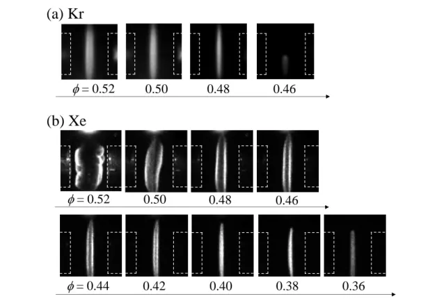
Figure 2 shows the experimental flame images during two typical experimental sequences at stretch rates a = 3.2 s-1. These images were taken from the high speed camera with
an image intensifier from the orthogonal direction to the burner axis. The dashed lines indicate the cylindrical burner outlet ports. The mixtures were ignited at higher equivalence ratios and the equivalence ratio was gradually decreased until extinction by keeping the stretch rate constant. For the Kr mixture (Fig. 2(a)), the flames are planar for equivalence ratios = 0.52–0.48. The image at = 0.46 for the Kr mixture was taken right before extinction resulting in a non-planar
Fig. 2 Experimental flame images at stretch rate a = 3.2 s-1 for Kr mixtures (a), and Xe
mixtures (b).
(b) Xe
= 0.52
0.50
0.48
0.46
0.42
0.40
= 0.52
0.50
0.48
0.46
0.38
0.36
(a) Kr
= 0.44
14 shape which will be discussed later. The flame is cellular and non-planar for the Xe mixture at = 0.52 and 0.50 (Fig. 2(b)). As the equivalence ratio decreases, the cellular flame becomes planar. The formation of the cellular flames for the Xe mixture is due to the occurrence of diffusive-thermal instability, attributed to the lower Lewis number of Xe mixtures (Le ≈ 0.5 for Xe mixtures, and Le ≈ 0.7–0.8 for Kr mixtures). The disappearance of the cells at lower equivalence ratios is in accordance with the previous study [13]. For Xe mixtures, the flames extinguish around = 0.38, which is much smaller than the equivalence ratio at extinction for the Kr mixture at the same stretch rate. This is due to the Lewis number effect. Similar to the experimental result for the Kr mixture, a non-planar flame was also observed for the Xe mixture just before extinction, which will also be discussed later.
15 The instantaneous flame images taken from different experimental sequences at = 0.48 for a = 3.2 and 2.1 s-1 with Kr mixtures, and for a = 3.2, 2.2 and 0.82 s-1 with Xe mixtures are
shown in Fig. 3. For Kr mixtures, the flames are planar at stretch rates a = 3.2 and 2.1 s-1. For the
case of a = 2.1 s-1, the flame is close to extinction. However, for the case of Xe mixtures, the
flames are planar at a = 3.2 s-1, but become cellular at a = 2.2 and 0.82 s-1. Particularly at a = 0.82
s-1, all the cells are separated which may lead to reactant leakage from the flame front to the
stagnation plane. These flames are called sporadic flames and have been reproduced by computations with the thermal-diffusion model in [12,13]. Here, the size of each cell in the radial direction is around 10 to 25 mm. Sporadic flames were not observed for Kr mixture flames for
Fig. 3 Experimental flame images at equivalence ratios = 0.48 and different stretch rates for (a) CH4/O2/Kr mixtures and (b) CH4/O2/Xe mixtures.
a = 3.2 s
-12.2 s
-10.82 s
-12.1 s
-1(b) Xe
(a) Kr
16 any conditions investigated in the current study.
To demonstrate the behavior of sporadic flames, flame images of sporadic flames at a = 0.82 s-1 and around = 0.39are shown in Fig. 4. Three ball-like flames are first formed at 5.8 s.
With passing time, the flame on the left-hand side inside the image extinguishes, while one ball-like flame remains at 8.8 s. The ball-ball-like flame pulsates and shifts which may be due to the asymmetric flame formation and the G-jitter. The ball-like flames survives for over 6 s until it is extinguished by the end of microgravity at around 12.3 s. The long lifetime of the sporadic flame experimentally indicates that sporadic flames are quasi-steady. However, longer microgravity duration is required to fully investigate the stability of such flames, characteristic lengths, and flame behaviors in the near future by space experiments scheduled for 2020 in the International Space Station.
Fig. 4 Experimental flame images of sporadic flames at equivalence ratios = 0.39 and stretch rate a = 0.82 s-1.
17 Other than the three flame types already introduced, i.e., planar flames, cellular flames, and sporadic flames, additional three types of flames were experimentally observed both for Kr and Xe mixtures. Typical flame images of these additional three flames for Xe mixtures are shown in Figs. 5(a), 5(b), and 5(c). Near the extinction of planar flames, planar circular flames with receding edges (Fig. 5(a)), and planar circular flames with propagating edges (Fig. 5(b)) were observed, in addition to the instantaneous whole region extinction. In Figs. 5(a) and 5(b), time = 0 corresponds to the time that the flame edges starts to move. For the flame shown in Fig. 5(a), the merged edges of the planar circular flame recedes into the burnt gas. The flames then extinguish approximately after 1.2 s from the time that the flame edges started to move. This corresponds to the failure wave of the flame edges. For the flame shown in Fig.5(b), the merged edges move towards the unburnt gas and propagates at 0.0–0.5 s. When the merged edges move toward the unburnt gas, local extinction occurs and the flame is broken into the core section and the fragments moving further downstream at 0.5 s in Fig. 5(b). Possible causes for the local extinction are the effect of radiation heat loss and the radial conductive heat loss [43,44]. From 0.6-1.3 s in Fig. 5(b), the behavior changes as the equivalence ratio is slightly decreased where the flame pulsates in the radial direction and extinguishes soon after 1.3 s. It should be noted that the detailed investigation on the mechanisms for this behavior could not be conducted since the
18 effect of local stretch acting on the flame edges may not be completely uniform depending on the flame location.
At high stretch rates, star-shaped flames were observed as shown in Fig. 5(c) for Xe flames at = 0.74 and a = 14.9 s-1. The image is taken from the HD camera placed in a diagonal
direction to the burner axis and the stagnation plane. The flame appears to have grooves along the stagnation plane, thus becoming star shaped. The flame also has wrinkles when seen from the direction along the stagnation plane although it is not shown here. The cause in the formation Fig. 5 Time history of the experimental flame images for CH4/O2/Xe mixtures. Planar circular
flames with receding edges at = 0.37 and a = 2.7 s-1 (a). Planar circular flames with propagating edges at = 0.35 and a = 3.2 s-1 (b). Star-shaped flames (c).
0.5
Fragments Core Section
0.7 0.9 1.1 1.3 0.3 0.1 0 = 0.33 = 0.35 Time (s)
(b)
0.5 0.7 0.9 1.1 1.3 0.3 0.1 0 Time (s) = 0.39 = 0.37(a)
Diagonal view Stagnation plane Burner Flow(c)
Trajectory of the flame edge19 mechanism of these flames are under consideration. Note that this is not due to flow turbulence since a planar flame was obtained with the same setup for CH4/O2/CO2 mixtures [14] and CH4/air
mixtures at the same and higher stretch rate region up to 15 s-1.
To compare with the experimental flame images, results obtained in the three-dimensional computations with the thermal-diffusion model using an overall one-step reaction
for counterflow flames are shown in Fig. 6. Here, temperature iso-surfaces at T = 0.75 and fuel concentration contours at X = 0 are shown. T = 0.75 is the location where approximately 30–50 % of the maximum heat release occurs in unstretched flames, which corresponds to the approximate location of the reaction zone. At = 0.234 and A = 0.26 which is equivalent to = 0.48 and a = Fig. 6 Temperature iso-surfaces at T = 0.75 and fuel concentration contours at X = 0. (a) Le = 0.75, = 0.234, A = 0.26, = 0.48, a = 1.0 s-1, (b) Le = 0.50, = 0.234, A = 0.26, = 0.48, a = 1.0 s-1, (c) Le = 0.50, = 0.234, A = 0.028, = 0.48, a = 0.11 s-1, (d) Le = 0.50, = 0.256, A = 0.028, = 0.42, a = 0.035 s-1. -20 0 20 0 -20 X 20 20 Z 0 -20 0 20 0 -20 20 X Y 20 -20 0 Z Z 20 -20 0 -20 0 0 -20 X Y 20 20 -20 0 20 0 -20 20 X Y 20 -20 0 Z
(a)
(c)
(d)
(b)
-20Le = 0.75
Le = 0.50
Mixture inlets Y X Z Flow direction20 1.0 s-1, planar flames are obtained for both Le = 0.75 and 0.50 conditions as shown in Figs. 6(a)
and 6(b). When the stretch rate is decreased, the flames extinguished from all zones at Le = 0.75 and A = 0.23 which is equivalent to 0.8 s-1, although it is not shown here. Whereas for Le = 0.50,
the flames become sporadic flames at = 0.234 and A = 0.028 which is equivalent to = 0.48 and a = 0.11 s-1, as shown in Fig. 6(c). Here, the cells formed by the diffusive-thermal instability
is split into separate ball-like flames, and reactant leakage from the gap between the cells to the stagnation plane is observed. Each cell splits or deforms, and is swept away due to the coupling effect of the diffusive-thermal instability and the velocity field. However, these sporadic flames are quasi-steady if the mean locations of flame propagation fronts are considered. This is supported by the fact that extinction for all of the cells were not observed even after 500 unit times equivalent to 131 s of computations in this condition, at = 0.234 and A = 0.028 equivalent to = 0.48 and a = 0.11 s-1. Figure 6(d) shows the temperature iso-surface and fuel concentration
contours at the same non-dimensional stretch rate (A = 0.028) with lower inlet fuel concentrations of = 0.256 than the condition in Fig. 6(c). With the decrease in the inlet fuel concentration from = 0.234 to = 0.256, the twin sporadic flames move closer together to form a single sporadic flame. The merging of sporadic flames is similar to the behavior of flame balls which stand closer than a critical distance [45]. At lower fuel concentrations of = 0.256, the gaps between each ball-like flame also become wider than the ones in = 0.234. The decrease in the distance between
21 the sporadic flames interposing the stagnation plane, and the increase in the gaps between ball-like flames with the decrease in the inlet fuel concentration is also in correspondence with the previous results of three-dimensional computations [12]. In this condition, computations were also continued for 800 unit times equivalent to 627 s without flame extinction inside the whole domain. It should be noted that flame extinction over the entire computational domain was observed with a slight decrease in the inlet fuel concentration ( = 0.260) at the same stretch rate (A = 0.028), or a slight increase in the stretch rate (A = 0.036) at the same inlet fuel concentration ( = 0.256).
5. Comparison between flame balls and sporadic flames
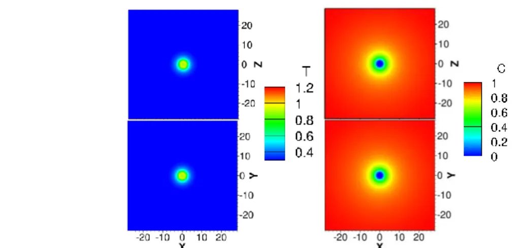
To compare the characteristics of sporadic flames with that of flame balls, three-dimensional computations were conducted for examining the single ideal flame ball by neglecting the convection term in the governing equations of the thermal-diffusion model. Figure 7 shows the temperature contours (left) and fuel concentration contours (right) on the X-Y plane along Z = 0 (top) and the X-Z plane along Y = 0 (bottom) at Le = 0.50 and = 0.256 equivalent to = 0.42. The result shown here is the solution at the steady state where the difference of the solution in time does not occur. The distance from the flame ball center to the point of maximum heat release rate is exactly the same in the X, Y, and Z-directions, and the center of the flame ball is located
22 very close to the origin of the coordinate. Thus, the current result can be regarded as an ideal spherical flame ball under the present parameters.
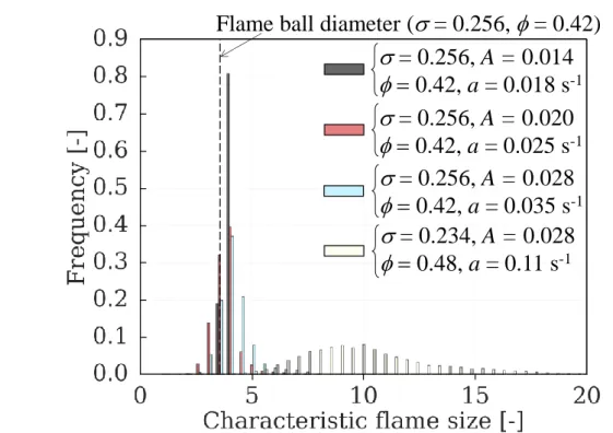
Fig. 8 shows the comparison between the computed characteristic length distributions of the sporadic flames and the flame ball diameter using temperature iso-surfaces at T = 0.75 as representations of the flames. The characteristic lengths of the sporadic flames were obtained by fitting ellipses by using the least square method [46] to the sporadic flames in the quasi-steady state viewed along the burner axis. Both the major length and the minor length of the ellipsoid were used. Only the sporadic flames in the region -28 ≦ X ≦ 28 and -28 ≦ Z ≦ 28 were used to eliminate the effect of the outlet boundary on the flames. Over 10000 measurements are typically present to make the size distribution for one condition. Also, the flames just before Fig. 7 Temperature contours (left) and fuel concentration contours (right) at Y = 0 (top) and Z = 0 (bottom) for Le = 0.50 and = 0.256 equivalent to = 0.42.
23 splitting were separated using the watershed algorithm [47]. As can be seen in Fig. 8, the size distribution of sporadic flames become narrower when non-dimensional stretch rate A becomes lower at constant . This is because the deformation of the ball-like flame before splitting becomes smaller and the rate of splitting for each ball-like flame becomes slower as A is decreased. At the same time, the size distributions of sporadic flames become closer towards the flame ball diameter with the decrease in A. In addition, the most frequently appearing sizes of the sporadic flames are larger than the flame ball diameter, but become slightly closer towards the flame ball diameter due to the shift in the size distribution with decreasing A. At A = 0.028 and different , the size distribution for sporadic flames become wider at smaller (higher ). This is due to the larger effect of the diffusive-thermal instability at smaller . At the same time, the size distribution and the most frequently appearing characteristic flame sizes of sporadic flames shift toward larger characteristic flame sizes. The increase in characteristic flame size with the increase in the mixture fuel concentration qualitatively agrees with the dependence of flame ball size to the mixture fuel concentration [32]. Here, the most frequently appearing characteristic flame size is around 9 equivalent to 2.1 cm, which agrees to our experimental results at the same equivalence ratio conditions. The behavior of characteristic flame size of the sporadic flames depending on the A and clearly indicate that sporadic flames are intermediate combustion modes that segue flame balls to propagating flames. Note that a stable flame ball solution at = 0.234 was not obtained
24 due to the three-dimensional instability [29,48,49].
Figure 9 shows the comparison between the flame structures at = 0.256 equivalent to = 0.42 for the counterflow planar flame at A = 0.26 equivalent to 1.0 s-1, sporadic flames at A =
0.028 equivalent to a = 0.035 s-1, and the flame ball. Here, the results along X = 0 and Z = 0 are
shown for the flame structures of the counterflow planar flame and the flame ball. The flame structures of sporadic flames are the result of eight measurements in the direction parallel to the burner axis near the center of the cells at different X, Z, and times. The figure shows that the
Fig. 8 Comparison between the distribution of the characteristic flame size for sporadic flames and the flame ball diameter.
Flame ball diameter (
= 0.256,
= 0.42)
= 0.256, A = 0.014
0.42, a = 0.018 s
-1
= 0.256, A = 0.020
0.42, a = 0.025 s
-1
= 0.256, A = 0.028
0.42, a = 0.035 s
-1
= 0.234, A = 0.028
0.48, a = 0.11 s
-125 sporadic flame structures have only small differences even at different locations and different times. In addition, the temperature profiles of sporadic flames are very close to the temperature profile of the flame ball, with the characteristic temperature profile of T 1/r in the preheat
zone where r is the distance from the flame center. This shows that the sporadic flame is heavily under the influence of diffusion, similar to flame balls. The fuel concentration profile of sporadic flames close to the stagnation plane are very similar to that of the flame ball close to the center of the flame ball. However, the fuel concentration profile at the location away from the center of
Fig. 9 Comparison of temperature and fuel concentration profiles for planar flames, sporadic flames, and flame balls at = 0.256 equivalent to = 0.42. Dotted line indicates the results of planar flames at A = 0.26 equivalent to 1.0 s-1, dashed and dotted lines indicate the result
of the flame ball, solid lines indicate the results for sporadic flames at A = 0.028 equivalent to a = 0.035 s-1.
0
0.2
0.4
0.6
0.8
1
1.2
0.0
0.2
0.4
0.6
0.8
1.0
1.2
-20
-15
-10
-5
0
T
em
per
at
ur
e
[-]
Fuel
con
cent
rati
on
[
-]
Location [-]
Sporadic
Flame
Counterflow planar flame
26 sporadic flames do not agree with that far from the center of the flame ball. This is due to the effect of the flow field. Figure 9 also shows that the distance between the location at the maximum temperature of the sporadic flame and the stagnation plane is smaller than the flame ball radius. Figures 8 and 9 show that the sporadic flames have slightly smaller characteristic flame sizes than the flame ball in the axial direction, but have larger characteristic flame sizes in the direction parallel to the stagnation plane.
6. Experimental and computational flame regime diagram
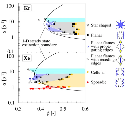
Figure 10 shows the experimental flame regimes, and the comparison between the experimental extinction points and the C-shaped extinction boundaries obtained by the one-dimensional computations using GRI-Mech 3.0 with the PREMIX-based code. The plots for the experimental flame regime indicate the boundaries between different flame types, i.e., extinction or transition into different flame types. Star-shaped flames are seen in both Kr and Xe mixtures at conditions above a certain stretch rate regardless of the equivalence ratio condition, which suggests that the star-shaped flames were not formed by the diffusive-thermal instability. In the experiments, sporadic flames are seen in only Xe mixtures. Planar flames, planar flames with propagating edges, planar flames with receding edges, and cellular flames are seen in both Kr and Xe mixtures. The region of cellular flames for Xe mixtures are larger than the one for Kr mixtures.
27 This further indicates that the cellular flame is formed by the diffusive-thermal instability. Near the limit of the planar flames, planar flames with propagating edges were seen at a > 3.0 s-1,
whereas planar flames with receding edges were seen at a < 3.0 s-1. This means that the
propagation direction of the edge of the planar flame changes depending on the stretch rate. Except the stretch rate conditions where star-shaped flames were observed, the experimental extinction points of Kr mixtures showed very good agreements with the C-shaped extinction boundary obtained by the one-dimensional computations with the PREMIX-based code using detailed chemistry. In these conditions, the equivalence ratio at extinction for the same stretch rate deviated within 0.01. In addition to the fact that the equivalence ratios at extinction for the airplane experiments with CH4/air mixtures agreed within ± 5 % to the results from the droptower
experiments for the same mixture by our previous study with the same setup [14], the experimental results are regarded to be reliable. However, for the Xe mixtures, there are large scatterings among the extinction points. For example, extinction was observed at = 0.35 and 0.41 for a = 1.9 s-1 in two different experiments. In these conditions, the near-limit flames were
planar flames with receding edges. Once these flames are formed, it is likely that the Lewis number effect and the large curvature of the flame before extinction acts to alter the deterministic nature of the steady deflagration wave. This leads to the large scattering of the extinction points for Xe mixtures. In addition, flame extinction was observed at = 0.43 and a = 1.1 s-1. However,
28 for a slightly lower stretch rate condition of a = 0.80 s-1, extinction was observed at = 0.37,
which is very different from the one-dimensional computational results of around = 0.50 at a = 0.8 s-1. In these conditions, sporadic flames were observed experimentally which indicate that the
formation of sporadic flames near the combustion limit caused the flame regime to extend far beyond the computational extinction boundary obtained by the one-dimensional computations
Fig. 10 Experimental flame regimes shown with the extinction boundaries (―) obtained by the one-dimensional computations with the PREMIX-based code using detailed chemistry for Kr and Xe mixtures. are star-shaped flames, ■ are planar flames, □ are planar flames with propagating edges, △ are planar flames with receding edges, ● are cellular flames, ●
are sporadic flames.
0.3
0.4
0.5
0.6
a
[s
-1]
Kr
1-D steady state
extinction boundary
[-]
a
[s
-1]
Star shaped
Cellular
Sporadic
Planar flames
with receding
edges
Planar flames
with
propa-gating edges
Planar
0.1
1
10
100
Xe
0.1
1
10
0.1
100
29 with the PREMIX-based code using detailed chemistry. This is the indication of the broken C-shaped extinction curve.
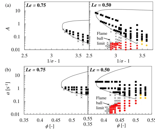
Figure 11 shows the computational flame regime diagram obtained in the three-dimensional computations with the thermal-diffusion model using an overall one-step reaction for counterflow flames in the dimensional and dimensional parameter values. In the non-dimensional regime diagram, the horizontal axis is plotted as a function of 1/1 since
1 / 1 /
1
Tb T0 can uniquely characterize the fuel concentration in the unburnt gas mixture.The flame types at either steady states or quasi-steady states are plotted in the flame regime diagram. The extinction boundary obtained by the one-dimensional computations with the thermal-diffusion model using an overall one-step reaction and the combustion limit of the flame ball obtained with the three-dimensional computations using an overall one-step reaction are also shown in Fig. 11.
30 At Le = 0.75 which is roughly equivalent to Kr mixtures in the experiments, only planar flames are formed and the computational extinction boundary obtained by the three-dimensional computations agree with that obtained by the one-dimensional computations. Since the extinction points obtained in the experiments and the three-dimensional computations agreed with the dimensional computations, it is both experimentally and computationally shown that the
one-Fig. 11 Computational flame regimes and the extinction boundaries (―) obtained by the three-dimensional and one-three-dimensional computations with the thermal-diffusion model using an overall one-step reaction in non-dimensional parameters (a) and dimensional parameters (b). ■ indicate planar flames, ● indicate cellular flames, ● indicate sporadic flames, × indicate extinction.
0.35
0.4
0.45
0.5
0.55
0.01
0.1
1
10
0.35
0.4
0.45
0.5
0.55
0.55
0.35
[-]
[-]
a
[s
-1]
Le = 0.75
Le = 0.50
Flame ball limit(b)
2.5
3
3.5
1/σ - 1
0.01
0.1
1
10
2.5
3
3.5
1/σ - 1
A
Le = 0.75
Le = 0.50
Flame ball limit(a)
31 dimensional modeling is sufficient to obtain the accurate extinction points for conditions around
Le = 0.75. Note that different behavior of the edges of the planar flames seen in the experiments
were not observed in the computations. This is likely due to the coupled effect of the initial condition, and the mixture being introduced along the entire computational boundary in the present computations. Neither cellular flames nor star-shaped flames are observed in the three-dimensional computations at Le = 0.75.
On the other hand, at Le = 0.50 which is roughly equivalent to Xe mixtures in the experiments, planar flames, cellular flames, and sporadic flames are observed in the three-dimensional computations with the thermal-diffusion model using an overall one-step reaction. Cellular flames are observed at relatively high equivalence ratio and low stretch rate conditions, which is in qualitative agreement with the experimental flame regime of cellular flames for Xe mixtures. Sporadic flames are seen at the conditions outside of the extinction boundary of the one-dimensional computations at A < 0.037 and > 0.415. The figure with the non-dimensional parameters showed the existence of a specific non-dimensional stretch rate limit in the region of sporadic flames which are in good correspondence with the observation in [12] and the theoretical prediction in divergent channels [26] that the flame propagation velocity of the sporadic flame remains almost constant regardless of the stretch rate. The region of the sporadic flame and the deviation of the C-shaped extinction boundary from the C-shaped extinction boundary in this
32 region qualitatively agrees to the experimental results. Interestingly, the lean combustion limit of the sporadic flame is very close to the lean combustion limit of the flame ball ( = 0.2583 equivalent to = 0.414) obtained with the three-dimensional thermal-diffusion model in the present computations. This indicates that the combustion limit of the sporadic flame may asymptote to the combustion limit of the flame ball. The upper Lewis number limit for flame balls were also around Le = 0.65 in the present computations. Since sporadic flames are the intermediate combustion modes between flame balls and propagating flames, the reason why the sporadic flames were not observed at Le = 0.75 is because the flame ball solution does not exist at Le = 0.75 for the current condition. For both Le = 0.75 and Le = 0.50 mixtures, quantitative agreement is not obtained between the experimental and the computational flame regimes. Possible causes include the interaction between the flame and the flow field, and the inaccuracy of the employed chemical model which may be a direction for investigations in the future.
7. Conclusions
In this study, experiments on counterflow flames for CH4/O2/Kr (Le ≈ 0.7–0.8) and
CH4/O2/Xe (Le ≈ 0.5) mixtures under microgravity were conducted to examine the effect of Lewis
number on the extinction boundary, flame regimes, and the formation of sporadic flames. Three types of computations were conducted, which are one-dimensional computations using detailed
33 chemistry with a PREMIX-based code, and three- and one-dimensional computations with the thermal-diffusion model using an overall one-step reaction, to compare with the experimental and computational results.
In the microgravity experiments at = 0.42, planar flames, cellular flames, and sporadic flames were observed with the decrease in stretch rate for Xe mixtures, while only planar flames were observed for Kr mixtures. The flame types obtained in the three-dimensional computations with the thermal-diffusion model using an overall one-step reaction for counterflow flames showed qualitative agreement to the experimental results at the same equivalence ratio conditions of = 0.42. In the microgravity experiments, planar circular flames with receding edges, planar circular flames with propagating edges, and star-shaped flames were observed.
Comparison between the sporadic flames obtained with the three-dimensional computations and the flame balls obtained with the same thermal-diffusion model showed that sporadic flames have slightly smaller characteristic flame sizes than the flame ball in the axial direction, but have larger characteristic flame sizes in the direction parallel to the stagnation plane. In addition, the stretch rate dependence of the characteristic flame size for sporadic flames, and the similarity in fuel concentration dependence of the characteristic flame sizes for sporadic flames and flame balls strongly indicated that sporadic flames are intermediate combustion modes that segue flame balls to propagating flames.
34 The extinction boundary in the experimental flame regime diagram for Kr mixtures showed qualitative agreement to the computational regime diagram at Le = 0.75. Also, the regime of cellular and sporadic flames and the extinction boundary in the experimental flame regime diagram for Xe mixtures showed qualitative agreement to the computational regime diagram at
Le = 0.50. The lean combustion limit of sporadic flames was shown to agree with that of the flame
ball. This indicated that the disappearance of the regime of sporadic flames for Le = 0.75 mixtures is due to the Lewis number limit of the flame ball, which was obtained to be around Le = 0.65 in the current conditions with the thermal-diffusion model.
8. References
[1] C.K. Law, S. Ishizuka, M. Mizomoto, Lean-limit extinction of propane/air mixtures in the
stagnation-point flow, Symp. (Int.) Combust. 18 (1981) 1791–1798.
[2] S. Ishizuka, C.K. Law, An experimental study on extinction and stability of stretched
premixed flames, Symp. (Int.) Combust. 19 (1982) 327–335.
[3] J. Sato, Effects of Lewis number on extinction behavior of premixed flames in a stagnation
flow, Symp. (Int.) Combust. 19 (1982) 1541–1548.
[4] S.H. Sohrab, C.K. Law, Extinction of premixed flames by stretch and radiative loss, Int.
35 [5] S.H. Sohrab, Z.Y. Ye, C.K. Law, Theory of interactive combustion of counterflow
premixed flames, Combust. Sci. Technol. 45 (1986) 27–45.
[6] C.J. Sung, C.K. Law, Extinction mechanisms of near-limit premixed flames and extended
limits of flammability, Symp. (Int.) Combust. 26 (1996) 865–873.
[7] K. Maruta, M. Yoshida, Y. Ju, T. Niioka, Experimental study on methane-air premixed
flame extinction at small stretch rates in microgravity, Symp. (Int.) Combust. 26 (1996)
1283–1289.
[8] J. Buckmaster, The effects of radiation on stretched flames, Combust. Theory Model. 1
(1997) 1–11.
[9] H. Guo, Y. Ju, K. Maruta, T. Niioka, F. Liu, Radiation extinction limit of counterflow
premixed lean methane-air flames, Combust. Flame. 109 (1997) 639–646.
[10] Y. Ju, H. Guo, K. Maruta, F. Liu, On the extinction limit and flammability limit of
non-adiabatic stretched methane–air premixed flames, J. Fluid Mech. 342 (1997) 315–334.
[11] K. Takase, X. Li, H. Nakamura, T. Tezuka, S. Hasegawa, M. Katsuta, M. Kikuchi, K.
Maruta, Extinction characteristics of CH4/O2/Xe radiative counterflow planar premixed
flames and their transition to ball-like flames, Combust. Flame. 160 (2013) 1235–1241.
[12] R. Fursenko, S. Minaev, H. Nakamura, T. Tezuka, S. Hasegawa, K. Takase, X. Li, M.
low-Lewis-36 number stretched premixed flames, Proc. Combust. Inst. 34 (2013) 981–988.
[13] R. Fursenko, S. Minaev, H. Nakamura, T. Tezuka, S. Hasegawa, T. Kobayashi, K. Takase,
M. Katsuta, M. Kikuchi, K. Maruta, Near-lean limit combustion regimes of
low-Lewis-number stretched premixed flames, Combust. Flame. 162 (2015) 1712–1718.
[14] T. Okuno, H. Nakamura, T. Tezuka, S. Hasegawa, K. Takase, M. Katsuta, M. Kikuchi, K.
Maruta, Study on the combustion limit, near-limit extinction boundary, and flame regimes
of low-Lewis-number CH4/O2/CO2 counterflow flames under microgravity, Combust.
Flame. 172 (2016) 13–19.
[15] L. Kagan, G. Sivashinsky, Self-fragmentation of nonadiabatic cellular flames, Combust.
Flame. 108 (1997) 220–226.
[16] I. Brailovsky, G.I. Sivashinsky, On stationary and travelling flame balls, Combust. Flame.
110 (1997) 524–529.
[17] L. Kagan, S. Minaev, G. Sivashinsky, On Disintegration of Cellular Flames, Lect. Notes
Comput. Sci. 2668 (2003) 811–818.
[18] F.A. Williams, J.F. Grcar, A hypothetical burning-velocity formula for very lean
hydrogen-air mixtures, Proc. Combust. Inst. 32 I (2009) 1351–1357.
[19] S. Minaev, L. Kagan, G. Joulin, G. Sivashinsky, On self-drifting flame balls, Combust.
37 [20] S.S. Minaev, L. Kagan, G. Sivashinsky, Self-propagation of a diffuse combustion spot in
premixed gases, Combust. Explos. Shock Waves. 38 (2002) 9–18.
[21] L. Kagan, S. Minaev, G. Sivashinsky, On self-drifting flame balls, Math. Comput. Simul.
65 (2004) 511–520.
[22] Y.L. Shoshin, L.P.H. d. Goey, Experimental study of lean flammability limits of
methane/hydrogen/air mixtures in tubes of different diameters, Exp. Therm. Fluid Sci. 34
(2010) 373–380.
[23] Y.L. Shoshin, J.A. Van Oijen, A. V. Sepman, L.P.H. De Goey, Experimental and
computational study of the transition to the flame ball regime at normal gravity, Proc.
Combust. Inst. 33 (2011) 1211–1218.
[24] F.E. Hernández-Pérez, B. Oostenrijk, Y. Shoshin, J.A. van Oijen, L.P.H. de Goey,
Formation, prediction and analysis of stationary and stable ball-like flames at ultra-lean
and normal-gravity conditions, Combust. Flame. 162 (2015) 932–943.
[25] Z. Zhou, Y. Shoshin, F.E. Hernández-Pérez, J.A. van Oijen, L.P.H. de Goey, Effect of
pressure on the lean limit flames of H2-CH4-air mixture in tubes, Combust. Flame. 183
(2017) 113–125.
[26] R. Fursenko, S. Minaev, Flame balls dynamics in divergent channel, Combust. Theory
38 [27] X. Chen, Z. Lu, S. Wang, Near limit premixed flamelets in Hele-Shaw cells, Proc.
Combust. Inst. 36 (2017) 1585–1593.
[28] Y.B. Zel’dovich, G.I. Barenblatt, V.B. Librovich, G.M. Makhviladeze, The Mathematical
Theory of Combustion and Explosions, Consultants Bureau, New York, 1985.
[29] J. Buckmaster, G. Joulin, P. Ronney, The structure and stability of nonadiabatic flame
balls, Combust. Flame. 79 (1990) 381–392.
[30] J.D. Buckmaster, G. Joulin, P.D. Ronney, The structure and stability of nonadiabatic flame
balls: II. Effects of far-field losses, Combust. Flame. 84 (1991) 411–422.
[31] C.J. Lee, J. Buckmaster, The Structure and Stability of Flame Balls: A
Near-Equidiffusional Flame Analysis, SIAM J. Appl. Math. 51 (1991) 1315–1326.
[32] J. Buckmaster, M. Smooke, V. Giovangigli, Analytical and numerical modeling of
flame-balls in hydrogen-air mixtures, Combust. Flame. 94 (1993) 113–124.
[33] M.S. Wu, J.B. Liu, P.D. Ronney, Numerical simulation of diluent effects on flame balls,
Symp. (Int.) Combust. 27 (1998) 2543–2550.
[34] M. Abid, M.S. Wu, J.B. Liu, P.D. Ronney, M. Ueki, K. Maruta, H. Kobayashi, T. Niioka,
D.M. Vanzandt, Experimental and numerical study of flame ball IR and UV emissions,
Combust. Flame. 116 (1999) 348–359.
39 of flame ball structure and dynamics, Combust. Flame. 116 (1999) 387–397.
[36] P.D. Ronney, Near-limit flame structures at low Lewis number, Combust. Flame. 82
(1990) 1–14.
[37] P.D. Ronney, M.-S. Wu, H.G. Pearlman, K.J. Weiland, Experimental study of flame balls
in space: Preliminary results from STS-83, AIAA J. 36 (1998) 1361–1368.
[38] Diamond Air Service Incorporation. http://www.das.co.jp/en/index.html (accessed
October 6, 2017).
[39] G.P. Smith, D.M. Golden, M. Frenklach, N.W. Moriarty, B. Eiteneer, M. Goldenberg, C.T.
Bowman, R.K. Hanson, S. Song, W.C. Gardiner Jr., V.V. Lissianski, Z. Qin, GRI-Mech
3.0, (2002). http://combustion.berkeley.edu/gri-mech/ (accessed October 6, 2017).
[40] NIST Chemistry WebBook, (2017). http://webbook.nist.gov/chemistry/ (accessed
October 10, 2017).
[41] W.J. Moore, Physical Chemistry, Tokyo Kagaku Dojin, Japan, 1974.
[42] T. Okuno, H. Nakamura, T. Tezuka, S. Hasegawa, K. Maruta, Ultra-lean combustion
characteristics of premixed methane flames in a micro flow reactor with a controlled
temperature profile, Proc. Combust. Inst. 36 (2017) 4227–4233.
[43] J.S. Park, D.J. Hwang, J. Park, J.S. Kim, S. Kim, S.I. Keel, T.K. Kim, D.S. Noh, Edge
40 (2006) 612–619.
[44] D.G. Park, J.H. Yun, J. Park, S.I. Keel, A study on flame extinction characteristics along
a C-curve, Energy and Fuels. 23 (2009) 4236–4244.
[45] Z. Lu, J. Buckmaster, Interactions of flame balls, Combust. Theory Model. 12 (2008) 699–
715.
[46] A.W. Fitzgibbon, R.B. Fisher, F. Hill, E. Eh, Direct Least Squres Fitting of Ellipses, IEEE
Trans. Pattern Anal. Mach. Intell. 21 (1996) 1–15.
[47] S. Beucher, C. Lantuéjoul, Use of Watersheds in Contour Detection, Rennes, France, 1979.
[48] W. Gerlinger, K. Schneider, H. Bockhorn, Numerical simulation of three-dimensional
instabilities of spherical flame structures, Proc. Combust. Inst. 28 (2000) 793–799.
[49] W. Gerlinger, K. Schneider, J. Fröhlich, H. Bockhorn, Numerical simulations on the