Bifurcation in a Generalized Frenkel Kontorova Model.

(1)

Bifurcations

in a

Generalized Frenkel Kontorova Model.

M. Peyrard

Laboratoire de Physique, Ecole Normale Sup\’erieure de Lyon,

₄₆

All\’ee d’Italie,

₆₉₃₆₄

Lyon C\’edex

07, France

$0$. M. Braun

Institute

_of

Physics UkrainianAcademy

_of

Sciences,

₄₆

ScienceAvenue, Kiev, UA-252022,

Ukraine

Abstract

Westudythegroundstateofa generalized Frenkel-Kontorova$(\mathrm{F}\mathrm{K})$ model

with a transverse degree offreedom. The model describes a lattice of atoms

interacting by long-range repulsive forces, which is submitted to a

two-dimensional substrate potential periodic in one direction and parabolic or

Toda-like in the transverse direction. When the magnitude of the interatomic

repulsion increases, the ground state of the model undergoes a series of

bifur-cations. In particular, the first bifurcationleads to a$\mathrm{z}\mathrm{i}\mathrm{g}$-zagground state and

results in drastic changeof system properties including a cusp in the average

elastic constant. The existence of the $\mathrm{z}\mathrm{i}\mathrm{g}$-zag state is fundamentally due to

the discreteness of the model. For incommensurate cases, the bifurcations

can interplay with the Aubry transition from a pinned to a sliding state so

that two different effects ofdiscreteness compete todetermine the properties

ofthe system.

I. INTRODUCTION

The standard Frenkel-Kontorova $(\mathrm{F}\mathrm{K})$ model describes a chain of particles interacting

by an harmonic potential and subjected to a sinusoidal on-site potential [1]. Besides its original aim ofmodeling crystal dislocations, the FK modelhas many applications in physics such as the description of magnetic domain walls, atoms adsorbed on a crystalline surface

or superionic conductors. When the interaction between the atoms is strong enough, a

continuum approximation can be used and the model reduces to the integrable Sine-Gordon

system. However, except for magnetic systems, the continuum limit is not valid for most physical applications. Discreteness effect may playafundamental role and modify drastically the properties of the system.

The standard FK model is a 1 space $+1$ time dimensional model with one degree of

(2)

transverse displacements of the atoms. A few attempts to generalize the model to $2+1$

dimensions have been made but they lead to complicated models that can only be studied numerically. Recently a generalized FK model has been introduced [2]. It is still a $1+1$

dimensionalmodel, but it has two degrees of freedom per site corresponding to longitudinal

and transverse displacements of the atoms. This generalized FK model has very interesting

properties because in this system lattice discreteness can play two different roles which compete against each other to determine the properties of the system as discussed below. Although the generalized FK model does not reduce to a known integrable model, because of its $1+1$ dimensional character an integrable system sufficiently close to it could perhaps

be found. Moreover the generalized FK model shows interesting mathematical properties, such as a sequence of bifurcations in its ground state, which could deserve the attention of mathematicians. There are many examples where models issued from physics have provided useful starting points for fundamental studies leading to results that the physicists could then use in their analysis of real systems. We hope that the generalized FK model, withits

richness, could perhaps become one additional example.

In section II we briefly review some properties of the standard FK model that are nec-essary to understand the properties of the generalized model. Section III introduces the generalized FK model and its ground state which shows a sequence of bifurcations when one model parameter is changed. Section IV shows how two different effects of the discrete nature of the model can compete to determine the properties of the system, and section V discusses some extensions and applications to physics.

II. THE STANDARD FK MODEL.

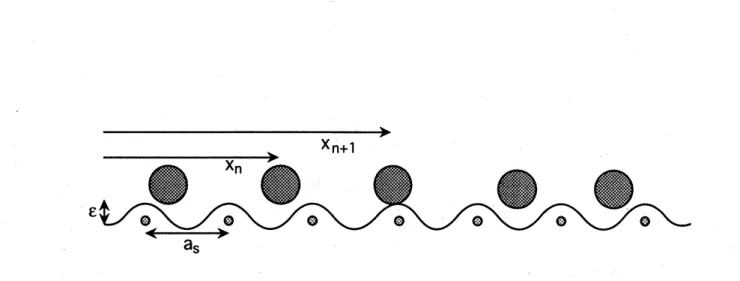
In order to understand the properties of the standard FK model, it is convenient to have in mind the case of a chain of atoms adsorbed on a crystal surface (Figure. 1). The hamiltonian of the system is

$H= \sum_{n}\frac{1}{2}m\dot{x}_{n}^{2}+V(_{X_{n+1^{-}}}x_{n})+Vs(X_{n})$ (1)

If it were alone, the coupling potential $V(x_{n+1}-x_{n})$ would impose an interatomic distance

$a_{A}$. The substrate potential $V_{s}(x_{n})$ has a period $a_{s}$. Let us consider for instance the case

$V(x_{n+1}-x_{n})= \frac{1}{2}(x_{n+1}-x_{n}-a_{A})^{2}$ and $V_{s}(x_{n})= \frac{1}{2}\epsilon[1-\cos(2TX_{n}/a_{s})]$ which reduces to

the integrable sine-Gordon model in the continuum limit. The ground state of the system

is obtained by minimizing the potential energy of the system. In terms of $\phi_{n}$ defined by $x_{n}=na_{S}+\phi_{n}$ whichmeasures the position of the $n^{\mathrm{t}h}$ atom with respect to the $n^{\mathrm{t}h}$ minimum

of the substrate $\mathrm{P}^{\mathrm{o}\mathrm{t}\mathrm{e}\mathrm{n}\mathrm{t}\mathrm{i}\mathrm{a}1}.$

’ the minimization of the potential

en.ergy,

leads to

$( \phi_{n+1}+\emptyset n-1^{-}2\phi n)-\epsilon\sin(\frac{2\pi}{a_{s}}\phi_{n})=0$. (2)

In the

c\’Ontinuum

limit,$\mathrm{V}\mathrm{a}\mathrm{l}\mathrm{i}\acute{\mathrm{d}}$

inthe strong coupling case when the coupling potential is much

larger.

than the substrate $\mathrm{p}\mathrm{o}.\dot{\mathrm{t}.}\mathrm{e}\mathrm{n}\mathrm{t}\mathrm{i}\mathrm{a}\mathrm{l}$, this equation is well approximated by the sine-Gordon $\mathrm{e}\mathrm{q}\mathrm{u}\mathrm{a}\mathrm{t}\mathrm{i}_{\mathrm{o}\mathrm{n}}.\cdot.$

(3)

FIG. 1. Aphysical system describedbythe standard FK model: atomson acrystalsurface. The

model describes aone dimensional chain ofatomsinteracting through a potential $v$, adsorbed on a

crystal surface that generates a substrate potential of period $a_{s}$. Only longitudinal displacements

of the atoms parallel to the surface are considered. The positions ofthe atoms are given by their

distance $x_{n}$ with respect to an origin $O$.

When the two distances $a_{A}$ and $a_{s}$ are commensurate, i.e. have a rational ratio, the ground state of the system is simple because it is periodic. The case of incommensurate

$a_{A}/a_{s}$ is more interesting. In this case discreteness plays a crucial role and is responsiblefor

a transition, known as the Aubry transition $[3,4]$, between two states of the system which have completely different properties. In order to understand the origin of this transition, it is convenient to replace Eq. (2) by a discrete mapping by defining $p_{n}=\phi_{n}-\phi_{n-1}$

.

It becomes

$=(_{p_{n}+}p_{n_{\emptyset\emptyset)}}+ \epsilon\sin(\frac{2\pi}{a_{s(}}\phi n)n+\epsilon\sin\frac{2\pi}{a_{S}}n)$ , (3)

which is known as the “standard map”. In the limit $\epsilonarrow 0$, where the coupling interaction

dominates, the standard map is in a non-chaotic domain. A diagram of $\phi_{n+1}$ versus $\phi_{n}$

(for varying $n$) shows a smooth closed curve (torus in the reduced phase space). In this

case, $\phi$ takes all the values in the range _{$[0, a_{s}]$}, indicating that there are atoms on tops

of the substrate potential _{maxima as well as in the minima, as schematized on fig. 2-a.}

Therefore the atomic chain is totally free to slide with respect to the substrate because

it costs the system no energy: some atoms go down the substrate potential maxima while others goup $[3,4]$. This is why this strong-coupling state of the FK model is called the sliding phase. If, on the contrary the substrate potential is large with respect to the interatomic

coupling, the atoms tend to fall into the minima of the substrate while the maxima are never

occupied as shown on the lower part of fig. 2-a. The torus of the diagram $\phi_{n+1}$ versus $\phi_{n}$

is broken into isolated islands and the atomic chain is now pinned to the substrate (hence

the name “pinned phase”) because its translation requires bringing atoms on the maxima of the substrate potential which costs energy. The difference between the sliding and the pinned state can also be detected in the spectrum of the small amplitude excitations of the ground state. In the sliding case the frequencies start at $\omega=0$, which corresponds to the translational mode of the system, while in the pinned phase the spectrum has a gap

(4)

occurs for awell defined value of$\epsilon=\epsilon_{c}$ which corresponds to the appearance of chaos in the standard map.

(a)

$\mathrm{v}_{0}$

FIG. 2. (a) Schematic picture of the positions of the atoms with respect to the substrate

potential on the two sides of the Aubry transition. The heavy line shows the occupied regions

of the potential. In the weak coupling $\mathrm{d}_{0}\mathrm{m}\mathrm{a}\mathrm{i}\mathrm{n}\mathrm{J}$

($\mathrm{t}\dot{\mathrm{o}}\mathrm{p}$ figure), the top part of the maxima are not

occupied. In thestrong coupling domain (lowerfigure), allregions, includingthe top of the barriers,

are occupied. (b) Schematic figureiuustrating the $\mathrm{p}_{\mathrm{o}\mathrm{S}\mathrm{s}\mathrm{i}}\mathrm{b}\dot{1}\mathrm{e}$ competition between the

$\mathrm{z}\mathrm{i}\mathrm{g}$-zag and

Aubry transitions (see Sec. IV). The threehorizontal lines correspond to three possible positions

of$g_{Aubry}$ with respect to the cusp in elastic constant $\mathrm{d}..\mathrm{u}\mathrm{e}\ddot{\mathrm{t}}\mathrm{o}$ thetransition to a $\mathrm{z}\mathrm{i}\mathrm{g}$-zag state.

III. GROUND STATE OF THE GENERALIZED FK MODEL.

A. Model

In addition to the atomic displacements parallel to the crystal surface, the generalized FK model considers also their displacements along the direction$y$ orthogonal to the surface.

The substrate potential, now written $V_{s}(\mathrm{r})$ with $\mathrm{r}\equiv(x, y)$, includes an additional term,

depending on $y$ which describes the confinement of the atoms in the vicinity of the surface.

We assume that $V_{s}(\mathrm{r})$ is the sum oftwo terms,

$V_{S}(\mathrm{r})=V_{x}(_{X})+V(yy)$, (4) where $V_{x}(x)$ is a periodic potential along the chain which is assumed to be sinusoidal as in

the standard FK model,

$V_{x}(x)= \frac{1}{2}\epsilon_{S}[1-\cos(2\pi x/a_{s})]$, (5)

and $V_{y}(y)$ is the confining potential in the transverse direction.

Two cases will be considered, a symmetric (even) potential $V_{y}(y)$ which is taken to be

parabolic,

(5)

where $\omega_{0y}$ is the frequency of a single-atom vibration in the transverse direction and $m_{a}$

the atomic mass, and a non-symmetric anharmonic potential which has been chosen with a Toda-like form

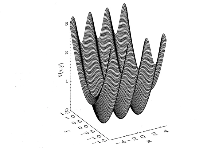
$V_{y}(y)=\omega_{0}yyanh[22(\exp-y/y_{anh})+(y/y_{anh})-1]$ (7) Figure 3 shows the shape of the substrate potential for a symmetric $V_{y}(y)$ potential.

FIG. 3. The two-dimensional substrate potential of the generalized FK model for a symmetric

confining potential $V_{y}(y)$.

It is convenient to use units such that the atomic mass is $m_{a}=1$, the amplitude of the periodic substrate potential is $\epsilon_{s}=2$ and its period is $a_{s}=2\pi$, so that the frequency of

longitudinal vibrations $\omega_{0x}=(\epsilon_{S}/2m)a\frac{1}{2}(2\pi/a_{S})$ is equal to 1.

For noninteracting atoms, the $x$ and $y$ degrees of freedom are decoupled due to the

simple form chosen for the substrate potential in$\mathrm{E}\mathrm{q}.(4)$. However theinteratomic interaction couples them. As long as the atoms use only an attractive branch of the interaction potential, the static properties of the model are equivalent to those of the standard FK model (but

the dynamics is modified). In a number of physical systems, however, the interatomic interaction is repulsive or has at least a repulsive branch. It can be due to Coulombrepulsion between ions in superionic conductors or between protons in hydrogen-bonded molecules,

(6)

or to Coulomb or dipole-dipole repulsion of atoms adsorbed on semiconductor or metal surfaces. We consider here the case of a Coulomb repulsion between the atoms

$V(r)=V_{0}/r$, (8)

where $V_{0}$ characterizes the amplitude of repulsion. Note that qualitative results do not depend on the specific form of $V(r)$ provided that the repulsion is concave, i.e. if $V(r)$

decreases monotonically with increasing distance $r$ between the atoms. Consequently, in

attempts to find an integrable model close to the generalized FK model, the exact form of the repulsive interaction could be changed. Since the Coulomb repulsion is a long range

interaction, the interatomic interaction is not restricted to nearest neighbors, as in the standard FK model, but extended to all atoms in the lattice.

For repulsive interactions the boundary conditions are essential to determine the proper-ties of the systembecause, with free boundaries, the chain of atoms would tend to decrease

its energy by expanding indefinitely. In a physical system, this is generally not possible and

for instance for atoms adsorbed on a surface, the average density of atoms is imposed by the experimental conditions. We represent this situation by imposing a fixed density of atoms. The chain consists of $N$ atoms distributed on the length $L=Ma_{S}=Na_{A}$, where $M$ is

the number of minima of $V_{x}(x)$ and $a_{A}$ is the mean interatomic distance along the chain.

Therefore the system is characterizedby the dimensionless concentration$\theta=N/M=a_{s}/a_{A}$ which is kept fixed in the limit $N,$ $Marrow\infty$. The density of atoms is constrained by using periodic boundary conditions with a period which is a multiple of $Na_{A}=Ma_{S}$. The total

potential energy of the system is

$U= \sum_{i=1}^{N}[V_{S}(\mathrm{r}_{i})+\frac{1}{2},\sum_{i=1}^{N^{*}}[V(|\mathrm{r}i-\mathrm{r}i+i’|)+V(|\mathrm{r}_{i}-\mathrm{r}_{ii}-’|)]]$ , (9)

where the index $\dot{i}$ labels the atoms, and the limit$N,$$N^{*}arrow\infty$ is assumed. Theground state

configuration corresponds to the absolute minimum of$U$. So to find the atomic coordinates

in the ground state $\{\mathrm{r}_{i}^{(0)}\}\equiv\{x_{i’ y_{i}^{(0)}\}}^{(0)}$, we look for static configurations by solving the set

of equations $\partial U/\partial x_{i}=0$, $\partial U/\partial y_{i}=0$, $\dot{i}=1,$$\cdots,$$N$, and then select the ground state

configuration which gives the absolute minimum of $U$.

When the ground state coordinates areknown, we canperform a linear stability analysis

by expanding linearly the equations of motion of the atomic chain and looking for the eigenfrequencies of the dynamical matrix. For commensurate cases ($\theta$ rational), the ground

state configuration is periodic and it is convenient to take the Fourier transform of the equations of motion which defines the frequencies $\omega_{j}(k)$ as a function of a wavevector $k$

belonging to the first Brillouin zone of the periodic lattice.

For a stable configuration all eigenfrequencies must be positive. When, for some model parameters, one of the frequencies vanishes, $\omega_{j}(k^{*})=0$, the corresponding configuration

be-comes unstable and evolves into a new configuration with the period $a^{*}=\pi/k^{*}$. The eigen-vector associated to the vanishing frequency determines the structure of the new ground state. This scenario corresponds to a continuous (second-order) phase transition.

More-over the model may also exhibit discontinuous (first-order) phase transitions when a model parameter (e.g., $V_{0}$ ) is changed. They occur when the energy of a metastable configura-tion becomes equal to the energy of the ground state configuration at a transition point

(7)

$V_{0}=V_{bif}^{(m)}$, and beyond this point the metastable and ground state configurations are

ex-changed.

As discussed in Sect. II, for the standard FK model, the average coupling energy is important because, for a given substrate in the incommensurate case, it determines whether the system is in a slidingor in a pinned phase. As the existence of the Aubry transition can be deduced from very general arguments comparing the coupling and the on-site potential

energies, we can expect it to occur in the generalized FK model too. Therefore it is useful

to calculate for each state the average elastic constant $g$ defined by

$g= \frac{1}{N}\sum_{i=1}^{N}gi$ , (10)

with

$g_{i}= \frac{1}{2},\sum_{=i1}^{N^{\mathrm{s}}}[\frac{\partial^{2}}{\partial x_{i}^{2}}(V(|\mathrm{r}i-\mathrm{r}i+i’|)+V(|\Gamma_{i}-\mathrm{r}i-i’|))]_{all0}\mathrm{u}=$ (11)

For the standard FK model$g$ defined by $\mathrm{e}\mathrm{q}\mathrm{s}$. (10) and (11) coincides with the dimensionless

coupling constant $(a_{S}^{2}/2\pi^{2}\epsilon)V\prime\prime(a_{s})$.

Most of the results of the present work have been obtained from a numerical analysis.

The ground state is obtained by a minimization of the potential energy of the system by

a relaxation procedure similar to the simulated annealing method to avoid the convergence

toward secondary minima [5]. In numerical calculations we can only take into account a

finite number$N^{*}$ of interacting neighbors. These neighbors cannot be simply chosen at the

starting of the calculation because, with transverse motions allowed, the sequence of the

atoms can change. Therefore we have to use a standard procedure of molecular dynamics,

i.e. select a cutoff distance $L^{*}(L^{*}\gg a_{A})$ and include in the calculation only the atoms

which are such that $r_{ii’}\leq L^{*}$.

In order to select the configuration with the lowest energy, we calculate the potential

energy per atom, $E$. Unfortunately, for the Coulomb interatomicrepulsion the total energy

ofinteraction depends on the cutoff distance $L^{*}$, and diverges as $\ln L^{*}$ in the limit $L^{*}arrow\infty$.

To avoid this problem, we subtract from the total potential energy a constant equal to the repulsion energy in the uniform configuration with the atomic coordinates $x_{i}=ia_{A},$ $y_{i}=0$.

Thus, each configuration is characterized by an energy

$E= \frac{1}{N}\sum_{i=1}^{N}[V_{S}(\mathrm{r}^{(0}i))\frac{1}{2},\sum_{1}^{L}V(ri,i+i’)+\frac{1}{2},\sum_{=i1}^{r}V(r_{i},i-i’)]+ri,i+i=i’<*t,i-i^{J<}L’-S(N_{m})V0/a_{A}$, (12)

where $S(N_{m})=1+ \frac{1}{2}+\frac{1}{3}+\cdots+\frac{1}{N_{m}}$ and $N_{m}=\mathrm{i}\mathrm{n}\mathrm{t}(L*/a_{A})$ .

B. The first bifurcation in commensurate states.

In the case of the standard FK model, for commensurate cases the ground state is almost trivial because it is periodic and can be obtained by solving a finite set of coupled nonlinear equations. For the generalized FK model, even for a commensurate case, the

(8)

situation is more interesting because, when $V_{0}$ reaches some critical value $V_{bif}$, the ground

state bifurcates from a state in which all the atoms are aligned with $y_{n}=0$ to a zig-zag state where atoms with positive and negative $y_{n}\neq 0$ alternate. An example is shown on

fig. 4-a. It should be noticed that this bifurcation is an intrinsically discrete property of the model. In a continuous model one cannot define such a $\mathrm{z}\mathrm{i}\mathrm{g}$-zag configuration.

FIG. 4. Example of bifurcation of the ground state of the generalized FK model in a

commen-surate case, $\theta=N/M=$ 16/32. Fig. (a) shows the transverse displacements $y$ of the atoms as

a function of the amplitude $V_{0}$ of the interaction potential. The inserts show schematically the

atomic positions on both sides of the bifurcation. Fig. (b) shows the averageelastic constant $g$ as

a function of$V_{0}$ for the same system.

Although the exact ground state configuration can only be obtained numerically for a

general commensurate state, in the simplest case of the commensurate concentration $\theta=$ $N/M=a_{s}/a_{A}=1/q$ with an integer $q$ such that the average interatomic distance $a_{A}$ is a

multiple ofthe lattice constant $a_{s},$ $(a_{A}=qa_{s})$, ananalytical determination of the bifurcation

point iseasy to obtain from the linear stabilityanalysis. In this case, for asmallinteratomic repulsion, the ground state is trivial (TGS), and all atoms are situated at the bottoms of the corresponding wells, $x_{i}^{(0)}=ia_{A}$ and $y_{i}^{(0)}=0$. The elementary cellof the system contains

one atom only, and the phonon spectrum consists of two branches (see fig. 5-a). The first

branch corresponds to motion along the $x$ direction,

$\omega_{1}^{2}(k)=\omega_{0x}+2\sum 2l=\infty 1V\prime\prime(laA)[1-\cos(klaA)]$, (13)

and the second branch to motion along the $y$ direction,

(9)

where $|k|\leq 1/2q$. Notice that the motions along the $x$ and $y$ directions are decoupled.

For repulsive interatomic interactions, $V’(la_{A})<0$ so that, when the magnitude of the

interatomic interaction increases, the frequency $\omega_{2}(k)$ decreases and reaches zero at some

criticalvalue $V_{0}=V_{bif}$. If theinteratomic repulsion decreases monotonically withincreasing

$r$ (i.e. if $V’$ is always negative), the first instability arises at the momentum $k=\pm 1/2q$.

The corresponding bifurcation value $V_{bif}$ can be determined from the equation

$\omega_{0y}^{2}+4\sum p=\infty 0\frac{V’[(2p+1)aA]}{(2p+1)a_{A}}=0$. (15)

In particular, for the Coulomb repulsion (8) $V_{bif}$ is equal to

$V_{bif}=\omega_{0}2ya_{A}^{3}/4C$, (16)

where $C\equiv\Sigma_{p=0}^{\infty}(2p+1)^{-3}=1.05179\cdots$

FIG. 5. Phonon spectrum of the commensurate trivial ground state for $\omega_{0y}=2$ at $V_{0}=V_{bij}$.

(a) $\theta=1/2(N^{*}=64),$ $V_{bif}=1886$ and (b) $\theta=5/7(N^{*}=60)V_{bif}=644.7$

.

In the case (b)

we usethe schemeof extended Brillouin zones.

Thus, for any monotonically decreasing interatomic repulsion the first bifurcation leads

always to a continuous transition from the trivial ground state to the zigzag- ground state with atomic coordinates $x_{i}^{\langle 0)}=ia_{A},$ _{$y_{i}^{(0)}=(-1)^{i}b$}. The amplitude$b$ ofthe transverse atomic

shifts is determined by the equation

$\omega_{0y}^{2}+4\sum_{l=0}^{\infty}V’(r_{l})/r_{l}=0,$ $r_{l}=[4b^{2}+a_{A}^{2}(1+2l)^{2}]1/2$. (17)

(10)

It will beconvenient to usehenceforthadimensionless amplitude of interatomicrepulsion

defined as $v=d/a_{A}$, where $d=(4b^{2}+a_{A}^{2})^{1/2}$ is the distance between the nearest neighbors in the ZGS, so that $v_{bif}=1$.

Toobtain analytical estimates, let us consider the case of a Coulomb repulsion restricted

to nearest and next nearest neighbors only. In this case the interaction is limited inside one

cell of the ZGS so that only $p=0$ has to be considered in $\mathrm{e}\mathrm{q}\mathrm{s}$. (15-17), and we get

$V_{bif}= \frac{1}{4}\omega_{0_{y}}^{2}a_{A}^{3}$, (18)

$b= \frac{1}{2}[(4V_{0}/\omega^{2}0y)^{2/3}-a_{A]}^{2}1/2$ , (19)

$d=(4V_{0}/\omega^{2}0y)1/3$, ₍₂₀₎ and

$v=(4V_{0}/\omega 20_{y}Aa^{3})1/3$ ₍₂₁₎

The average elastic constant (10) for the TGS is equal to

$g_{(\tau cs)}= \frac{9}{4}\frac{V_{0}}{a_{A}^{3}}$, (22) while for the ZGS it is determined by the expression

$g_{(Zcs})= \frac{1}{16}\omega_{0_{y}}^{2}(v^{3}$\dagger $12/v-24)$ . (23)

According to Eqs.(22) and (23), the elastic constant $g$ for the TGS increases linearly with $V_{0}$ up to the value_{$g_{bif}=9\omega_{0y}^{2}/16$}. But after the bifurcation

$g$ decreases, reaches the local

minimum $gmin=4.705\omega_{0y}/216\sim 0.5gbiJ$ at $v=8^{1/5}$, and then rises again.

Figure4-b shows the numerical results for $\theta=\frac{1}{2}$ and $\omega_{0y}=2(N=16, M=32)$, taking into account the interaction of a large number of neighbors $(N^{*}=64)$. The results are in

agreement with the predictions ofthe simpleapproach described above. Note that the cusp of the elastic constant $g$ at the bifurcation point $V_{bif}$ explains many remarkable properties

of the model, as discussed in Sect. III.

The properties of the system with a complex, but commensurate, elementary cell are similar to the properties found above for a simple unit cell with only one atom. Let us

consider arationalatomic concentration $\theta=s/q$, where$s$ and $q$ arerelativelyprime integers,

and $s<q$ so that there is not more than one atom in one well of the longitudinal substrate

potential. The ground state of the system is still periodic, with period $sa_{A}=qa_{S}$, and for

$V_{0}$ below the bifurcation point, the

$\mathrm{g}\mathrm{r}\mathrm{o}$

, und state is again a trivial ground state with $y=0$

for all atoms. Their $x$ positions along the chain are now shifted from the minima of the

potential wells and these shifts increase with $V_{0}$. The elementary cell of the TGS consists now of $s$ atoms. Therefore, the phonon spectrum has to have $2s$ branches as shown in fig.

5-b where for clarity we use the scheme of extended Brillouin zones so that the momentum

$k$ varies in therange $|k|\leq k_{\theta},$ $k_{\theta}=sk_{B}=\theta/2$ with $k_{B}=\pi/sa_{A}=1/2q$ being the boundary

of the first Brillouin zone in our units where$a_{s}=2\pi$. Fig. 5-b shows that the first instability arises again at $k=\pm k_{\theta}$, and it corresponds to a continuous transition from the TGS to the

(11)

C. Higher-order bifurcations.

Taking into account long rangeforces and not only nearest neighbor interactions, allows further bifurcations beyond the first instability leading to the ZGS.

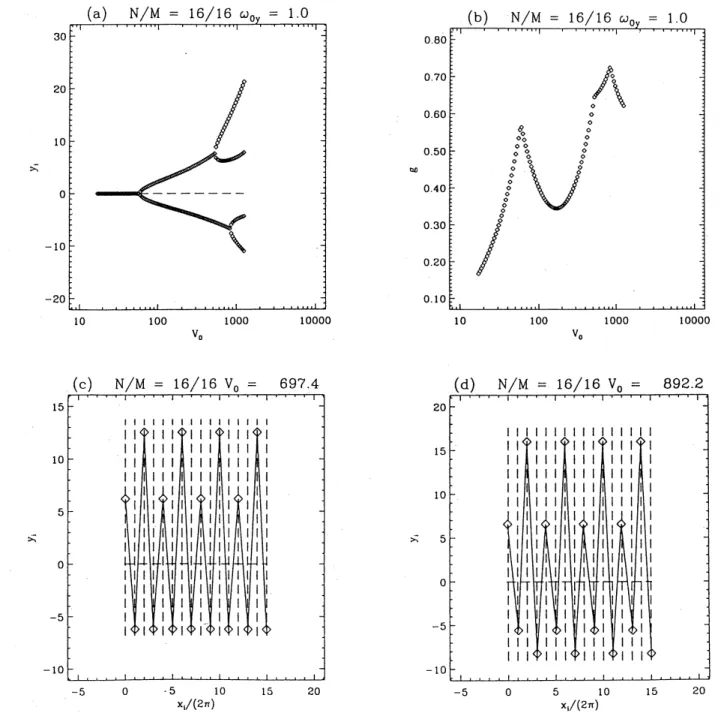
FIG. 6. Transverse atomic displacements (a) and elastic constant $g$ versus $V_{0}(\mathrm{b})$, and two

typicalconfigurationsfor$V_{0}=697(\mathrm{c})$and $V_{0}=892(\mathrm{d})$ forthe Toda transverse substrate potential. $\theta=1$ ($N=M=16$ and $N^{*}=64$), $\omega_{0y}=1,$ $yanh=20$.

(12)

The simplest situation is observed for a non symmetric confining potential $V_{y}(y)$ such as

the Toda potential of Eq. (7). Figure 6 shows one examplefor the simplest commensurate situation $\theta=1$. Three bifurcations can be observed. Each new bifurcation induces a cusp

in the average elastic constant as shown on fig. 6-b. After the first bifurcation the positive and negative transverse displacements of the atoms are not thesame, in agreement with the asymmetry of the potential, i.e. the resulting $\mathrm{z}\mathrm{i}\mathrm{g}$-zag ground state is no longer symmetric

with respect to $y=0$. It is easyto get a qualitative understanding of the second bifurcations

by viewing the $\mathrm{z}\mathrm{i}\mathrm{g}$-zag ground state as a combination of two “chains”, the upper

sub-chains corresponding to atoms having a positive displacements and the down sub-chain to atoms having a negative displacement. Since the interactions are not restricted to first neighbors, atoms in a sub-chain interact with each other in asimilarmanner as the atoms in the original chain. One can mentally isolate one of the sub-chains, the role of the second one being simply to create a local minimum around the $y$ value of the sub-chain that we chose

to study. It is then possible to consider the linear stability of the chosen sub-chain. The analysis is very similar to that of the total chain if we include the effect of the second

sub-chain, assumed to stay fixed, as an external potential, and we again find that the sub-chain

tends to bifurcate into a (

$‘ \mathrm{s}\mathrm{u}\mathrm{b}- \mathrm{Z}\mathrm{i}\mathrm{g}-_{\mathrm{Z}}\mathrm{a}\mathrm{g}$

” _{configuration. Such a configuration can be observed}

on fig. 6-c. For a higher value of $V_{0}$ the down sub-chain becomes unstabletoo and bifurcates in a sub-zig-zag structure as shown on fig. 6-d.

The bifurcation points are determined by the curvature of $V_{y}(y)$ for $y$ equal to atomic

coordinates in one sub-chain. To find the bifurcation points, we can deduce, similarly to $\mathrm{E}\mathrm{q}.(18)$, an equation

$V_{bif}^{(m)}= \frac{1}{4}(\omega_{eff}^{()3})m2(2m-1)aA$ , (24)

where we have introduced $\omega_{efj}^{2}$ $=$ $[ \frac{\partial^{2}}{\partial y^{2}}V_{sub}(r)]_{r}=r$

: instead of

$\omega_{0y}^{2}$. Because $\omega_{eff}^{2}$ $=$

$\omega_{0y}^{2}\exp(-\beta y)$for the Todapotential (7), we see that the upperand down sub-chainsare now

characterized bydifferent effectivefrequencies$\omega_{eff}^{up}$ and$\omega_{eff}^{d_{ow}n}$ such that$\omega_{eff}^{up}<\omega_{0y}<\omega_{eff}^{d_{ow}n}$.

So the instability arises first at $V_{0}=V_{bif}^{(up)}$ in the upper sub-chain, and it leads to creation

of a subzigzag ground state configuration in the upper sub-chain only (fig. 6-c). Then, at

$V_{0}=V_{bif}^{(\mathit{0}}dwn)>V_{bif}^{(p)}u$, the down sub-chain becomes unstable, creating a subzigzag

configu-ration in the$\mathrm{d}\mathrm{o}\mathrm{W}\mathrm{n}- \mathrm{S}\mathrm{u}\mathrm{b}-_{\mathrm{C}}\mathrm{h}\mathrm{a}\mathrm{i}\mathrm{n}$too (fig 6-d). Thus, the second bifurcation leads tosplitting of

the $\mathrm{t}\mathrm{w}\mathrm{o}^{-}\mathrm{s}\mathrm{u}\mathrm{b}$-chain structure into a $\mathrm{t}\mathrm{h}\mathrm{r}\mathrm{e}\mathrm{e}- \mathrm{S}\mathrm{u}\mathrm{b}-_{\mathrm{C}}\mathrm{h}\mathrm{a}\mathrm{i}\mathrm{n}$configuration, then into a$\mathrm{f}_{\mathrm{o}\mathrm{u}}\mathrm{r}-_{\mathrm{S}\mathrm{u}}\mathrm{b}-_{\mathrm{C}}\mathrm{h}\mathrm{a}\mathrm{i}\mathrm{n}$

configuration. We could thus expect that the evolution of the ground state configuration would proceed in an analogous manner: additional bifurcations could start on the top

sub-chain leading to the creation of the next sub-zigzag structure (i.e., the next splitting of the

top sub-chain), and then this splitting would spread sequentially to sub-chains with smaller

$y$ values. This scenario reminds of the well-known Feigenbaum picture for the transition

from a regular to the chaotic behavior, so it should end at some accumulation point by the creation of an incommensurate structure for a rational $\theta$.

The picture discussed above is however oversimplified because the distance between the central sub-chains (i.e. the sub-chains with the smallest transversaldisplacements) does not increase fast enough, and the interaction between them increases with $V_{0}$. Therefore they

(13)

are very difficult to observe numerically, and, as shown in fig. 6 we have seen only 3 bifurcations (leading to the splitting of the system into 4 sub-chains) in our calculations.

The case of a symmetric confining potential $V_{y}(y)$, which may seem simpler because of

the additional symmetry, turns out to be more complicated, because the top and down sub-chains become unstable for the same value of the repulsive interaction $V_{0}$. Since a system close to an instability is very sensitive to small perturbations, the instability of each sub-chain affects the other. A separate _{study of one sub-chain can no longer lead to useful}

results and the study of the full system is required. An analytical linear stability analysis is however possible in the simple case $\theta=1$ if we consider only nearest and next nearest

neighbor interactions [5]. Because the zigzag configuration for $\theta=1$ has two atoms in the

elementarycell,the phonon spectrumconsists of four branches $\omega_{j}(k),$$j=1$ to 4. Contrary to

the case of the TGS, in the ZGS $x$ and $y$ modes are coupled. In order to find an instability

point $v_{\mathrm{c}rii}$, we have to take the lowest root $\omega_{\min}(k)=\min_{j}\omega_{j}(k)$ and then look for the point

where $\omega_{\min}(k)$ reaches zero for the first time at some _$k=k^{*}$. The analysis of the spectrum

shows that the instability of the $\mathrm{z}\mathrm{i}\mathrm{g}$-zag configuration occurs through afirst order transition

in which a state which was metastable becomes the minimum energy configuration. Thus, beginning from the ZGS, the ground state of the system undergoes a series of first-order transitions with increasing interatomicrepulsion.

These predictions are based on analytical expressions in the case $\theta=1$ with only nearest

and next nearest interactions. They should be checked by numerical calculations. However

the _{calculations become very difficult because, for complicated structures, it is} _very _difficult

to make surethat wehaveobtained the true ground_{state after relaxation. Therefore we have}

limited our investigations to a few particular situations without attempting an exhaustive

study which would have been of limited physical interest because the perfectly symmetric

potential is an idealized case.

IV. AUBRY TRANSITIONS

Asmentioned above, sincetheAubry transitionofthe standard FK modelcan be deduced

from general argumentson the competition between the on-sitepotential and theinteratomic coupling, one can expect to _{find it in the generalized FK model too. The question which}

arises naturally is to what extent the introduction of a transverse degree of freedom in our

model can _{affect the Aubry transition. The answer can be derived from the variation of the}

elastic constant $g$ versus $V_{0}$ obtained in the previous section. Because the bifurcation point $V_{bif}$is determined by the curvatureofthe transverse substratepotential,

$V_{bij}\propto\omega_{0y}^{2}$ according

to $\mathrm{E}\mathrm{q}.(18)$ while the Aubry transition concerns essentially the longitudinal displacements, the relative positions of the two transitions can change depending on model parameters.

Depending on the value of $\omega_{0y}^{2}$, we can predict three different scenario for the behavior of

the system with increasing $V_{0}$ as shown schematically on fig. 2-b.

(a) The case of $\omega_{0y}$ below a first threshold $\omega^{*},$ $\omega_{0y}<\omega^{*}$, such that _{$V_{bif}<V_{Aubry}$} (case 1

on fig.2). _{In this case the Aubry transition will not occur because the first bifurcation, to}

a $\mathrm{z}\mathrm{i}\mathrm{g}$-zag state, which reduces the effective interatomic coupling, occurs before

$g$ can reach

the magnitude $g_{Aubry}$ required for the Aubry transition. Taking $g_{Aubry}\simeq 1$ for the golden

mean $\theta_{g.m}$. and $g_{bif}\simeq 9\omega_{0y}^{2}/16$, the value $\omega^{*}$ can be estimated as

(14)

(b) The case of large $\omega_{0y},$ $\omega_{0y}>\omega^{**}$ (where

$\omega**\mathrm{i}\mathrm{s}$ a second characteristic value)

,

for

which$V_{bif}\gg V_{Aubry}$ and$g_{Aubr}y<gmin \equiv\min g(V_{0})$ for all$V_{0}$within the ZGS (case2 on figure

2). In this case the Aubry transition is observed when $V_{0}$ reaches $V_{Aubry}$ and the bifurcation

which occurs later does not bring any qualitative change in the system behavior because the minimum of $g$ after the bifurcation is above $g_{Aubr}y$. Only a higher order bifurcation

could bring a qualitative change. Taking $gmin\simeq 0.5g_{bif}$, the value $\omega^{**}$ can be estimated as

$\omega^{**}\approx 4\sqrt{2}/3\approx 1.9$ for $\theta=\theta_{g.m}.\cdot$

(c) For intermediate $\omega_{0y},$ $\omega^{*}<\omega_{0y}<\omega^{**}$ (

$\mathrm{c}\mathrm{a}\mathrm{S}\mathrm{e}3$ on fig. 2), when $V_{0}$ is increased, the system undergoes first an Aubry transition in which the pinned ground state is transformed to a sliding ground state. But then the bifurcation to a $\mathrm{z}\mathrm{i}\mathrm{g}$-zagstate can reduce the average

elastic constant below $g_{Aubry}$. The system undergoes a reverse Aubry transition and the

lattice gets pinned to the substrate again. The further increase of$g$ which occurs after the

minimum can cause again a direct Aubry transition restoring the sliding state, at least up

to the second bifurcation.

In order to check numerically these predictions, we should in principle chose $N/M$

ir-rational, which is not possible for a finite system because $M$ and $N$ must be integers in

our calculations. There are however sequences of rational numbers which approach closely

an irrational number. They can be obtained from the continuous fraction expansion of the irrational number. An example is provided by the Fibbonacci sequence

$1 arrow\frac{2}{3}arrow\frac{3}{4}arrow\frac{5}{7}arrow\frac{8}{11}arrow\frac{13}{18}arrow\frac{21}{29}arrow\frac{34}{47}arrow\cdots$ , (25)

which tends to $\theta_{g.m}’$

. $=(3+\sqrt{5})/(5+\sqrt{5})$, equivalent to the golden mean for the Aubry

transition. We chose $N=34,$ $M=47$, and $N^{*}=34$ in our study. Note, however, that in

a numerical simulation the value $\theta$ is always rational, so the ground state will stay slightly

pinned.

To simulate the intermediate case (c), which corresponds to the most interesting

situa-tion, we take $\omega_{0y}=1.5$ which is in the range estimated above, $4/3<\omega_{0y}<4\sqrt{2}/3$. The

results are presented in fig. 7. The Aubry transition takes placebefore the bifurcation, and

then $g$ continues to

$\mathrm{r}\mathrm{i}\mathrm{s}\dot{\mathrm{e}}$

to the value $g_{bif}=$ 1.189 (see fig. 7-b). But after the bifurcation which takes place at $V_{bij}=381$, the elastic constant $g$ decreases and reaches the minimum

$gmin=0.771$ whichis lower than $g_{Aubry}$ at $V_{0}=1079$. Figure 7 shows that, in the vicinity of

the minimum of the function $g(V_{0})$, the atomic displacements decrease strongly and thereis

not any more an atom on top of the maxima of $V_{x}(x)$, as expected (see fig. 2-a). Thus, in

theregion near the minimum of$g(V_{0})$ the ground state seems again pinned. A sensitivetest

of the existence of the Aubry transitions is providedbythe calculation of the linear response of the atomic chain to an external force $F$ applied to all the atoms, along the direction of

the $x$ axis. We calculate the mean shift of the atoms, $\triangle x_{S}hijt=(1/N)\Sigma_{i=1}N(x_{i}-xi)(0)$, with

respect to their positions without the force, $x_{i}^{(0)}$, and define a susceptibilityas

$\chi=\triangle x_{shift}/F$. (26)

We expect $\chiarrow\omega_{0x}^{-2}$ in the limit $V_{0}arrow 0$, and $\chiarrow\infty$in the sliding state. The behavior of the

susceptibility(fig. 7-c) attests that we have observed the predicted reverse Aubry transition from the sliding to the pinned state at $V_{0}=578$ when $g=$ 0.898. With further increase

(15)

when $g=782$ the system undergoes a second direct Aubry transition before the second bifurcation.

$.\simarrow$

$\mathrm{v}_{0}$

FIG. 7. (a) Longitudinal displacements $\triangle x$ of the atoms with respect tothe nearest

minimum

of$V_{x}(x),$ $(\mathrm{b})$ transverse displacements _$y,$ $(\mathrm{c})$ inverse susceptibility $\chi^{-1}$ versus $V_{0}$ forthe

incommen-suratestructure $(\theta=34/47, N^{*}=34)$for$\omega_{0y}=1.5$. Theinverse susceptibility shows the existence

(16)

V. CONCLUSION

The generalized FK model, in which a transverse degree of freedom has been added to the usual longitudinal motions, is an interesting example of a nonlinear lattice with more than one degree of freedom per unit cell. From the mathematical point of view, very little is known for such systems, particularly when discreteness is important. The properties of the generalized FK model show however that they deserve interest, in spite of the analytical difficulties, for two reasons. First the model exhibits a very rich behavior even when one considers only the static properties of the ground state. We found for instance a sequence of bifurcations that could perhaps lead to a chaotic (glass-like) spatial structure of the ground state while, for the standard FK model, if chaotic states can exist in the discrete

case, they never correspond to the ground state of the system. The richer behavior of the

generalized FK model arises from the coupling of several instabilities (the instabilities of the different sub-chains). The generalized FK shows also an example where discreteness is crucial (we would not have a $\mathrm{z}\mathrm{i}\mathrm{g}$-zag state without discreteness) and can play several

competitive roles to determine the structure of incommensurate systems. Moreover the dynamics of the commesurate generalized FK model exhibits interesting features such as

different types of soliton-like excitations in the $\mathrm{z}\mathrm{i}\mathrm{g}$-zag state [2]. The second reason for the

interest of the generalized FK model lies in its various applications in physics, in particular

to describe atoms adsorbed on surfaces, epitaxial crystal growth and surface diffusion [6].

The model can for instance reproduce the reconstruction ofthe first layer, observed in some

cases of epitaxial growth, when the second layer begins to grow [6]. It can also explain

some observations of anomalously fast diffusion of atoms on surfaces by showing how some

extra atoms added to afilled first layer can generatemetastabledefects which are extremely

mobile [6].

Although the generalized FK model is significantly more complicatedthan the standard FK model because it has been built with complex physical applications in mind, it is still tractable due to its one-dimensional character which allows analytical studies in some

par-ticular cases. From a mathematical point of view, it would be worthwhile to look for the

simplestmodel that would preserve themain features ofthe generalized FK model discussed

here while allowing more complete theoretical studies.

ACKNOWLEDGMENTS

$\mathrm{M}.\mathrm{P}$. would like to thank S. Takeno and S. Homma for the opportunity of a long term

visit in Japan which made possible his participation in this conference.

This work was supported in part by the NATO Linkage Grant LG 930236. One of us

($\mathrm{O}.\mathrm{M}$.B.) was partially supported by the Soros Grant awarded by the American Physical

Society (and by a Grant of the Ukrainian State Committee for Science and Technology).

The main part of this work has been done during a stay of $\mathrm{O}.\mathrm{M}$.B. at the Ecole Normale

Sup\’erieure de Lyon and it has been completed during a visit of M.P at the Institute of Physics of Kiev. Both authors want to acknowledgeawarm hospitality in theseinstitutions.

(17)

REFERENCES

[1] Ya. Frenkel and T. Kontorova, 1938, Phys. Z. Sowietunion 13, 1; Zh. Eksp. Teor. Fiz. 8,
89.
[2] O.M. Braun and Yu.S. Kivshar, 1991, Phys. Rev. B44, 7694; O.M. Braun, O.A.
Chubykalo, Yu.S. Kivshar, and L. V\’azquez, 1993, Phys. Rev. B48, 3734.
[3] S. Aubry, 1983, Physica D7,240.
[4] M. Peyrard and S. Aubry, 1983, J. Phys. C16, 1593.
[5] O.M. Braun and M. Peyrard, Phys. Rev. E51, 4999 (1995) [6] O.M. Braun and M. Peyrard, Phys. Rev. B51,17158 (1995)