列車の走行によって引き起こされるトンネル内の音場
大阪大基礎工 杉本信正 (Nobumasa SUGIMOTO)
ABSTRACT
This paper deals with a sound field in a tunnel generatedby traveling of a
high-speed train. A magnitude of pressure disturbances is estimated by using the
linear acoustic theory. Thetrain’s motion is taken into account through asource
term of the wave equation in the form of a pair of acoustic monopoles or an
acoustic dipole. One-dimensional analysisis first given for two cases. One is the
sound field generated by the impulsive motion of the train in an infinitely long tunnel and the other is the one by the entry motion into a semi-infinite tunnel. The magnitude of the pressure pulse radiatedis derived on assuming the source
strength averaged over the tunnel’s cross-section. To justify this assumption, the three-dimensional analysis is developed for the impulsive motion of the dipole
alongthe axis of the tunnel of circular cross-section. The sound fieldis solvedin
aclosed form and this solution endorses the results basedon theone-dimensional analysis.
1. Introduction
When a high-speed train travels inside of a long tunnel, it happens that pressure
dis-turbances generated give rise to an acoustic shock wave even if the train speed is well
subsonic. As this shock wave is radiated from a tunnel exit, it brings about an
environ-mental noise problem just like the one due to a sonic boom by supersonic flight. This
problem becomes severer with increase in train speed so it will be vitally important for
magnetically levitated trains whose project is now underway. The radiation of the shock
wave is not the only problem. Emergence of the shock wave itself is undesirable, of course,
for durability and performance of trains as well as tunnels. To inhibit the shock wave,
the author has proposed to connect an arrayof Helmholtz resonators, more generally, an
array of cavities along the tunnel as side branches and has demonstrated its effectiveness
by the numerical simulations (Sugimoto, 1992, 1993).
This paper considers, onreturning to the startingpoint of the problem, a sound field in
a tunnel generated bytraveling ofatrain to estimate a maximumpressure level. Because
the train speed is well subsonic, evolution of pressure disturbances may be treated in a
framework of the acoustic theory. It is assumed to consist of the following three stages.
The first stage is an inner flow field rather than a sound field around the train in which
pressure
disturbances from the flow field are radiated in the form of sound but the linearacoustic
theory is still applicable to the lowest approximation. This is the region withwhich
thepresentpaper is concerned. Thefinal stageis a far sound field in which the shockwave emerges. Evolution in this fieldcannot be described appropriately without invoking
the nonlinear theory. The results in the near field are to be employed in prescribing the
pressure
disturbances for further evolution in the far field.2. Modeling of the problem
Before embarking on analysis, we discuss how the problemis modeled. First of all, we
note that atrain is such a slender and stremlined body that it has an extremelylong axial
dimension relative to alateral one. In fact, the train stretches axially from about 20 to a
few hundred meters against the lateral dimension, say, 3 $m$
.
Here we define a ‘long train’and a (short train’ according as the train’s axial length is much longer than the tunnel’s
typical diameter or comparable with it. Similarly, the tunnel has also an extreme ratio
of axial length to diameter. The following analysis
assumes
along tunnel so no effects ofreflection at the tunnel exit are taken into account.
When thetraintravelsin the tunnel, it gives rise to pressure disturbances inthe vicinity
of the train. Because of the extremely slender geometry, twofold length-scales are
associ-ated with the flow field, i.e., the train’s length $l$ and the tunnel’s diameter $D$
.
Here thetrain’s lateral dimension $s$ is small relatively to $D$ but is regarded as being comparable
with it. With the train speed $U$ as a typical one, two time-scales are therefore involved,
$l/U$ and $D/U$
.
Because the train speed is slower than the sound speed $a$ (for example,$U$ is assumed to be 150 $m/s(540km/h)$ for the magnetically levitated trains so that the
train’s Mach number $M(=U/a)$ is 0.44), the flow field is weakly compressible so that its
effect may still be neglected to the lowest approximation with respect to the Mach
num-ber. In fact, the magnitude of pressure fluctuations is small relative to the atmospheric
one. Such a region is identified as the inner flow field.
With distances away from the train, the pressure disturbances are radiated in the
form of sound. As its typical wavelength is of course
the.
train’s length, a typicaltime-scale is determined by the sound speed to be $l/a$
.
With $l$ ranging from 20 to a fewhundred meters long, this time is long enough as sound that the pressure disturbances
fall under the category of so-called infra-sound. In fact, their frequency spectra observed
for the present high-speed train (Shinkansen) are below 10 Hz. This near sound field is
characterized as follows. The tunnel plays a role ofa waveguide sothat the sound can be
propagated without any geometrical spreading. The waveguide allows the sould field to
be representedby asuperposition ofthe lowest non-dispersive mode and higher dispersive
modes. Since the group velocity of the higher mode is slower than the sound speed, the
plane toward the far field.
For this near field, the effect of the inner flow field is taken into account through a
source term of the linear wave equation as follows (Crighton et al., 1992):
$\frac{\partial^{2}p}{\partial t^{2}}-a^{2}\triangle p=a^{2}\frac{\partial q}{\partial t’}$ (1)
where $p$ and $q$ denote, respectively, the excess pressure over the atmospheric pressure $p_{0}$
and the source term reflecting the near flow field; $\triangle$ stands for the three-dimensional
Laplacian, $t$ being the time. The train’s motion creates the mass outflow in front and
. the inflow of the same magnitude at rear. At the
same
time, the train’s motion exertsforce to the surrounding fluid, i.e., air. Since the train is not acoustically compact axially
but compact laterally, its motion may be modeled by distribution ofpoint sources along
a finite axial extent. But a long train having a small lateral dimension may be modeled
substantially by a pair of the acoustic monopoles of strength $\rho_{0}SU$ but with opposite
sign where $\rho_{0}$ is the density of the fluid in equilibrium and $S$is the train’s cross-sectional
area. In unbounded $s$pace, the pair of the moving monopoles defines the slender Rankine
ovoid provided the distance between the monopoles is long enough, so that an effect of
the tunnel wall becomes weaker as $s$ becomes smaller.
As opposed to the long train, the short train may be modeled by an acoustic dipole.
The dipole strength is given by the sumof themomentum $\rho_{0}SUl$as if the fluid displaced
by the train were moving with $U$ and the impul$se$ imparted to the fluid (Lighthill, 1986).
The impulse is also the momentum associated with the virtual mass of the train. For
the Rankine ovoid, the virtual mass in the axial direction is given by $2\pi\rho_{0}s^{3}/3$, where
$s$ is now taken to be the radius of the cylindrical part in the middle of the ovoid. But
this mass is negligibly small compared with that of the displaced fluid $\pi\rho_{0}s^{2}l$
.
Even fora short train with $l=20m$ and $s=1.5m$, the fraction of the virtual mass in the dipole
strength is as small as 5%. Thus the impulse may be neglected. Even if the dipole is
assumed, it does not necessarily mean a sphere, for which the dipole strength is given by
$3\rho_{0}V/2(=2\pi\rho_{0}s^{3})$ where $V$ is the volume ofthe sphere of radius $s$
.
In the following, the one-dimensinal version of Eq.(l) is first solved by taking, as the
source term, a pairof monopoles with opposite sign andthen a dipole. It is assumed that
the source strength can be averaged over the tunnel’s cross-section so that the monopole
strength and the dipole strength are taken to be $\rho_{0}\chi U$ and $\rho_{0}\chi Ul$, respectively, where $\chi$
denotes the ratio ofthe train’s cross-sectional area to the tunnel’s one. We then solve the
sound field for two cases, one inwhich the train moves impulsively with constant speed in
an infinitely long tunnel and the other in which the train rushes into a semi-infinitely long
tunnel. The maximum pressure level in each case is derived. To justify the averaging, a
three-dimensional sound field is solved by taking the case of the impulsive motion ofthe
3. $One- dimensional$ analysis
Let us first examine a sound field due to the impulsive motion of a one-dimensional
monopole in an infinitely long tunnel. The sound field due to a pair of the monopoles can
easily be constructed by the principle ofsuperposition. The pressure field is governed by
the following equation:
$\frac{\partial^{2}p}{\partial t^{2}}-a^{2}\frac{\partial^{2}p}{\partial x^{2}}=a^{2}\frac{\partial}{\partial t}[mh(t)\delta(x-Ut)]$, (2)
where $m$ designates the monopole strength $\rho_{0}\chi U$ and $h(t)$ and $\delta(x-Ut)$ denote,
respec-tively, the unit step function and the delta function, $x$ being the axial coordinate
along
the tunnel. Executing the differentiation in the source term, it consists of two parts,
$m\delta(t)\delta(x-Ut)and-mUh(t)\delta’(x-Ut)$ where the prime implies the differentiation with
respect to the argument. The former represents the impulsive effect while the latter
represents the steadily moving effect.
Upon introducing new coordinates $\xi(=x-Ut)$ and $\tau(=t),$ $Eq.(2)$ can be solved by
using the Fourier transform with respect to $\xi$ and the Laplace transform with respect to
$\tau$ defined, respectively, as follows:
$\hat{p}=\frac{1}{(2\pi)^{1/2}}\int_{-\infty}^{\infty}p(\xi, \tau)e^{ik\xi}$ df and $\tilde{p}=\int_{0}^{\infty}p(\xi, \tau)e^{-\sigma\tau}d\tau$. (3)
Then Eq.(2) is transformed into
$\tilde{\hat{p}}=\frac{ma^{2}}{(2\pi)^{1/2}}\frac{(\sigma+iUk)}{\sigma[(\sigma+iUk)^{2}+a^{2}k^{2}]}$ (4)
Effecting the respective inverse transforms and reverting to the original variables $x$ and
$t,$ $p$, designated as$p+m$’ is obtained as
$p_{+m}= \frac{ma}{2}[-\frac{1}{1-M}h(x-at)+\frac{1}{1+M}h(x+at)+\frac{2M}{1-M^{2}}h(x-Ut)]h(t)$. (5)
The pressure field due to the positive and negative monopoles positioned by the axial distance$l$ apart can be derived byadding to (5),
$P-m$ with$x$replaced by$x+l$
.
Theresultingpressure field is shown in Fig.1. The positive square pulse ofmagnitude $ma/[2(1-M)]$
is propagated into the positive direction of $x$ with the sound speed, while the negative
pulse of $magnitude-ma/[2(1+M)]$ is propagated into the negative direction. Also the
negative pulse ofmagnitude $maM/(1-M^{2})$ is moving with the train. With $m=\rho_{0}\chi U$,
the magnitude of the positive pressure pulse $\Delta p_{+}$ is given relative to the atmospheric
pressure $p_{0}$ as follows:
$\frac{\triangle p_{+}}{p_{0}}=\frac{ma}{2(1-M)p_{0}}=\frac{\gamma}{2}\frac{\chi M}{(1-M)})$ (6)
Figure 1: Pressure field duetothe impulsivemotion ofthe pair of the monopolesinthe infinitely long tunnel where the bold solid line shows the total pressure profilewhile the broken lines show
the pressure profiles due to each monopole located at $x=0$ and $x=-l$ at $t=0$, respectively,
and the dotted lines are the paths of the train’s head and tail.
negativepulse propagatinginto thenegative directionis provided by (6) with the Doppler
factor $1-M$ replaced$by-(1+M)$
.
Also the magnitude of the negative pulse $\Delta p_{0}$ movingwith the train is given by
$\frac{\triangle p_{0}}{p_{0}}=-\frac{\gamma\chi M^{2}}{1-M^{2}}$
.
(7)If the limit $larrow 0$ is taken with $ml(=\mu)$ fixed, the pressure field due to the impulsive
motion of the dipole can be derived. With the source terms $q=-\mu h(t)\delta’(x-Ut)$, the
solution is easily obtainable by differentiating (5) with respect to $x$ and changing the sign
as follows:
$p= \frac{\mu a}{2}[\frac{1}{1-M}\delta(x-at)-\frac{1}{1+M}\delta(x+at)-\frac{2M}{1-M^{2}}\delta(x-Ut)]h(t)$
.
(8)The pressure field is given just as in Fig.1 with each square pulse replaced by the delta
function of the corresponding strength. Once the solution due to the dipole is known, it
can be extended to the case with the pair of monopoles. Then the delta function may be
regarded not only as the limit of the square pulse but also as that of various sequences of
appropriate functions such as the following Gaussian function:
$\delta(x)=\lim_{larrow 0}\frac{1}{l}\exp[-(\frac{x}{l/\sqrt{}\pi}I^{2}]\cdot$ (9)
Next we consider the sound field due to the entry of the train into the semi-infinite
tunnel extending in$x\geq 0$
.
In this case as well, we first consider the case of the monopolemoving with constant speed $U$
.
Unlike the preceding case, the monopole strength doesnot change with time so the source term $q$ is taken as $m\delta(x-Ut)$
.
Rather the boundaryFigure 2: Pressure field due to the entry motion of the pair of the monopoles into the
semi-infinitely long tunnel in $x\geq 0$ where the bold solid line shows the total pressure profile and the
dotted lines are the paths of the train’shead and tail.
obtained as
$p_{+m}= \frac{mU}{1-M^{2}}\{-h[M(x-at)]+h(x-Ut)\}$
.
(10)Combining $p+m$ and $p_{-m}$ due to the negative one with $t$ shifted to $t-l/U$ this time,
the sound field is shown in Fig.2. The positive square pulse of width $al/U$, lengthened
eventually by the factor $a/U(=1/M)$ due to a delay in the entry time of the negative
source, is propagated with the sound speed and the negative pulse of the same magnitude
but ofwidth $l$ is moving with the train. Themagnitude of the positive pulse
$\triangle p_{+}$ relative
to$p_{0}$ is given by .
$\frac{\Delta p_{+}}{p_{0}}=\frac{mU}{(1-M^{2})p_{0}}=\frac{\gamma\chi M^{2}}{1-M^{2}}$
.
(11)Ifthe limit $larrow 0$ is taken again with $ml(=\mu)$ fixed for the dipole, $p$ is given by
$p= \frac{\mu U}{1-M^{2}}\{\delta[M(x-at)]-\delta(x-Ut)\}$
.
(12)Here the argument of the first deltafunction implies that the pulse width is lengthened.
Because $\delta$[$M$(x–at)] $=M^{-1}\delta(x-at)$, its integral is increased by the factor $M^{-1}$
.
4. Three-dimensional analysis
The one-dimensional analysis rests cruciallyon the assumption thatthe source strength
can be averaged over the tunnel’s cross-section. In order to justify this assumption, we
along the axis of the infinitely long tunnel of circular cross-section. With the radial
coordinate $r$, Eq.(l) becomes on assuming the axisymmetry and taking $\mu=\rho_{0}SUl$
$\frac{\partial^{2}p}{\partial t^{2}}-a^{2}(\frac{\partial^{2}p}{\partial r^{2}}+\frac{1}{r}\frac{\partial p}{\partial r}+\frac{\partial^{2}p}{\partial x^{2}}$ $=-a^{2} \frac{\partial}{\theta t}[\mu h(t)\delta(r)\frac{\partial}{\partial x}\delta(x-Ut)]$ , (13)
with the boundary condition on the tunnel wall at $r=R$:
$\frac{\partial p}{\partial r}=0$ on $r=R$
.
(14)(17)
Introducing$\xi$and$\tau$defined as before and effecting the Laplace and the Fourier transforms,
it follows that
$( \frac{d^{2}}{dr^{2}}+\frac{1}{r}\frac{d}{dr}-\beta^{2})\hat{p}\sim=-\frac{\mu(\sigma+iUk)ik}{(2\pi)^{1/2}\sigma}\delta(r)$, (15)
with $\beta=[(\sigma+iUk)^{2}+a^{2}k^{2}]^{1/2}/a$
.
For $0<r<R,\tilde{\hat{p}}$ can easily be solved as$\tilde{\hat{p}}=c_{1}I_{0}(\beta r)+c_{2}K_{0}(\beta r)$, (16)
with unknown constants $c_{1}$ and $c_{2}$ where $I_{n}$ and $K_{n}$ (with $n=0$) stand, respectively,
for the modified n-th order Bessel function of the first and the second kind. As will
be used later, in passing, $J_{n}$ denotes, of course, the n-th order Bessel function of the
first kind. Imposing the boundary condition (14), we derive $c_{1}=c_{2}K_{1}(\beta R)/I_{1}(\beta R)$
.
The inhomogeneous equation (15) is satisfied by integrating it over a small circular disk
centered at $r=0$ and making use of the divergence theorem applied to the disk of unit
axial thickness. Noting the asymptotic form of$K_{0}(\beta r)\sim-\log r$ as $rarrow 0,$ $c_{2}$ is found to
be $(2\pi)^{-3/2}\mu(\sigma+iUk)ik/\sigma$
.
With $c_{1}$ and $c_{2}$ thus determined, $p$ is obtained by evaluatingthe following inverse transforms:
$p= \frac{\mu}{4\pi^{2}}\int_{-}^{\infty_{\infty}}dke^{-ik\xi}\{\frac{1}{2\pi i}\int_{Br}\frac{(\sigma+iUk)ik}{\sigma}[\frac{K_{1}(\beta R)}{I_{1}(\beta R)}I_{0}(\beta r)+K_{0}(\beta r)]e^{\sigma\tau}d\sigma\}$ ,
where $Br$ stands for the Bromwich path.
Theinverse Laplacetransform isfacilitatedby introducingauxiliarypaths alongcircular
arcs of infinite radius and invoking the Cauchy’s integral theorem. Because the integrand
has the branch points at $\beta=0$, i.e., at $\sigma=i(a-U)k$ and $-i(a+U)k$, and $\beta=\infty$,
the branch cuts are introduced in the $\sigma$-plane as shown in Fig.3 where the cuts extend
from the branch points to infinity in parallel with the nagative axis. Defining $\beta$ so as
to take a positive value along the imaginary axis between the branch points, $\beta$ takes
asymptotically $\sigma/a$ on the arcs $C_{0},$$C_{1}$ and $C_{3}$ and takes $-\sigma/a$ on $C_{2}$
.
Examining anasymptotic form of the integrand over the infinite arcs (see e.g., Watson, 1958), it is
found that for $0<\tau<r/a$, the Bromwich path is closed by $c_{0}$ so that $p$ vanishes. For
$r/a<\tau$, on the other hand, the path is closed by the arcs on the left-hand half plane
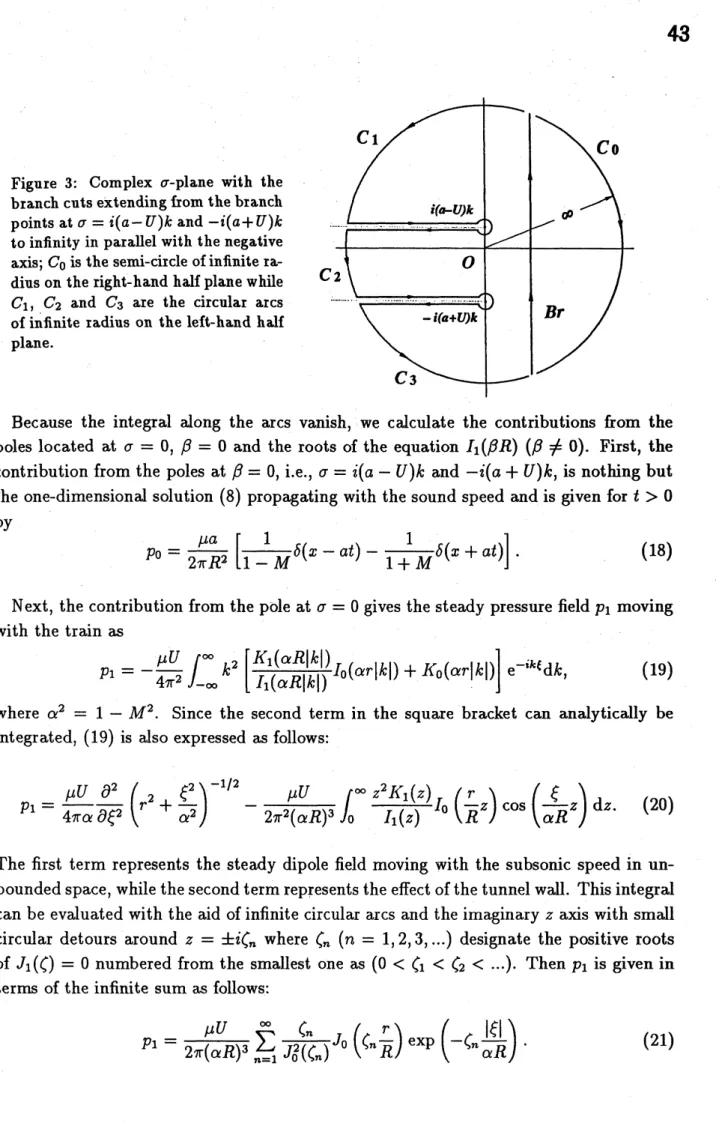
Figure 3: Complex $\sigma$-plane with the
branch cuts extending from the branch pointsat $\sigma=i(a-U)kand-i(a+U)k$
toinfinityin parallel with thenegative axis; $C_{0}$isthesemi-circle of infinite
ra-diusonthe right-handhalf plane while
$C_{1},$ $.C_{2}$ and $C_{3}$ are the circular arcs
of infinite radius on the left-hand half
plane.
Because the integral along the arcs vanish, we calculate the contributions from the
poles located at $\sigma=0,$ $\beta=0$ and the roots of the equation $I_{1}(\beta R)(\beta\neq 0)$
.
First, thecontribution from the poles at $\beta=0$, i.e., $\sigma=i(a-U)kand-i(a+U)k$, is nothing but
the one-dimensional solution (8) propagating with the sound speed and is given for $t>0$
by
$p_{0}= \frac{\mu a}{2\pi R^{2}}[\frac{1}{1-M}\delta(x-at)-\frac{1}{1+M}\delta(x+at)]$
.
(18)Next, the contribution from the pole at $\sigma=0$ gives thesteady pressure field $p_{1}$ moving
with the train as
$p_{1}=- \frac{\mu U}{4\pi^{2}}\int_{-\infty}^{\infty}k^{2}[\frac{K_{1}(\alpha R|k|)}{I_{1}(\alpha R|k|)}I_{0}(\alpha r|k|)+If_{0}(\alpha r|k|)]e^{-*k\xi}dk$, (19)
where $\alpha^{2}=1-M^{2}$
.
Since the second term in the square bracket can analytically beintegrated, (19) is also expressed as follows:
$p_{1}= \frac{\mu U}{4\pi\alpha}\frac{\partial^{2}}{\partial\xi^{2}}(r^{2}+\frac{\xi^{2}}{\alpha^{2}})^{-1/2}-\frac{\mu U}{2\pi^{2}(\alpha R)^{3}}\int_{0}^{\infty}\frac{z^{2}K_{1}(z)}{I_{1}(z)}I_{0}(\frac{r}{R}z)\cos(\frac{\xi}{\alpha R}z)dz$
.
(20)The first term represents the steady dipole field moving with the subsonic speed in
un-boundedspace, while the second termrepresentsthe effect ofthe tunnel wall. Thisintegral
can be evaluated with the aid of infinite circular arcs and the imaginary $z$ axis with small
circular detours around $z=\pm i\zeta_{n}$ where $\zeta_{n}(n=1,2,3, \ldots)$ designate the positive roots
of $J_{1}(\zeta)=0$ numbered from the smallest one as $(0<\zeta_{1}<\zeta_{2}< )$
.
Then $p_{1}$ is giveninterms of the infinite sum as follows:
The third contribution results from the roots of $I_{1}(\beta R)=0$
.
The roots $\beta R=\pm i\zeta_{n}(n=$$1,2,3,$ $\ldots$) correspond to $\sigma=\sigma_{n}^{\pm}=-iUk\pm i\omega_{n}$with
$\omega_{n}=a(k^{2}+\zeta_{n}^{2}/R^{2})^{1/2}$ where the sign
$\pm is$ understood to be vertically ordered hereafter. Then the residue of each pole in the
inverse Laplace transform is given by
$\pm\frac{a^{2}}{R^{2}}\frac{(\sigma_{n}^{\pm}+iUk)k}{\sigma_{n}^{\pm}J_{0^{2}}(\zeta_{n})\omega_{n}}J_{0}(\zeta_{n^{\frac{r}{R}}})\exp(\sigma_{n}^{\pm}\tau)$
.
(22)Noting that the factor $\sigma_{n}^{\pm}+iUk$ implies the differentiation with respect to $t$, the third
contribution$p_{2}$ is evaluated as follows:
$p_{2}= \frac{\mu\partial}{4\pi^{2}R^{2}\partial t}[\sum_{n=1}^{\infty}\frac{1}{J_{0^{2}}(\zeta_{n})}J_{0}(\zeta_{n^{\frac{r}{R}}})\Phi_{n}(\xi, \tau)]$ , (23)
with $\Phi_{n}=\Phi_{n}^{+}-\Phi_{n}^{-}$ where $\Phi_{n}^{\pm}$ are defined by
$\Phi_{n}^{\pm}=\int_{-\infty}^{\infty}\frac{a^{2}k}{\sigma_{n}^{\pm}\omega_{n}}\exp(\sigma_{n}^{\pm}\tau-ik\xi)dk$
.
(24)Using the definitions of$\sigma_{n}^{\pm},$ $\Phi_{n}$ are rewritten in the following form:
$\Phi_{n}=\int_{-\infty}^{\infty}\frac{2aMk^{2}}{\alpha^{2}\kappa_{n}^{2}\omega_{n}}\sin(\omega_{n}t)\exp(-ikx)dk-\int_{-}^{\infty_{\infty}}\frac{2ik}{\alpha^{2}\kappa_{n}^{2}}\cos(\omega_{n}t)\exp(-ikx)dk$
,
(25)with $\kappa_{n}^{2}=k^{2}+\zeta_{n}^{2}/\alpha^{2}R^{2}$
.
For $at<|x|$, these integrals can be evaluated analytically(Oberhettinger, 1957). It follows that
$\Phi_{n}=-\frac{2\pi}{\alpha^{2}}$(sgn x)$\exp[-\zeta_{n}\frac{(x-Ut)sgnx}{\alpha R}]$ , (26)
so that
$p_{2}=- \frac{\mu U}{2\pi(\alpha R)^{3}}\sum_{n=1}^{\infty}\frac{\zeta_{n}}{J_{0^{2}}(\zeta_{n})}J_{0}(\zeta_{n^{\frac{r}{R}}})\exp(-\zeta_{n}\frac{|\xi|}{\alpha R})$
.
(27)For $|x|<at$, on the other hand, $\Phi_{n}$ is alternatively expressed as
$\Phi_{n}=\frac{2\pi M}{\alpha^{2}}J_{0}(\eta)-\frac{\pi M\zeta_{n}}{\alpha^{3}R}\int_{-at}^{at}J_{0}(\eta’)\exp(-\zeta_{n}\frac{|x-x’|}{\alpha R})dx’$
where $\eta$ and $\eta’$ are defined, respectively, as $\zeta_{n}(a^{2}t^{2}-x^{2})^{1/2}/R$ and $\zeta_{n}(a^{22’}t-x^{2})^{1/2}/R$
.
Finally the contribution from the integral along the branch cuts vanishes because the
jump across the cut cancels out as a whole of the square bracketin (17). Thus the integral
(17) is evalutated to be the sum
$p=p_{0}+p_{1}+p_{2}$
.
(29)It is immediately seenthatfor $at<|x|,$ $p_{1}$ and$p_{2}$ cancel outso that $p$vanishes, namely, an
undisturbed region prevails. At the wavefront $|x|=at,$ $p$ is given by the one-dimensional
solution $p_{0}$
.
As the factor $\mu/\pi R^{2}$ indicates $\rho_{0}\chi Ul$, it is justified that the strength canbe averaged over
(the
tunnel’s cross-section. For $|x|<at,$ there appear the dispersivedisturbances $p_{2}$ in addition to the steady pressure field $p_{1}$ expressed in terms of the
infinite sum of the discrete higher modes. In this paper, we pause here to present only
the solution $p_{1}$ and $p_{2}$ in the closed form.
5. Discussions
When a train starts suddenly with constant speed in a long tunnel or when a train
rushes into a tunnel, the rapid change gives rise to the radiation of the pressure pulse
forward. Its magnitude in the near field has been evaluated by solving the linear wave
equationwith the sourceterm of the pair of monopoles or of thedipole. For the impulsive
motion, the magnitude (6) isproportional to the Mach number $M$ rather than $M^{2}$ except
for the Doppler factor $1-M$
.
For the entry motion, by contrast, the magnitude (11)is proportional to $M^{2}$
.
The magnitude for the impulsive motion is found to be greaterthan that for the entry motion. In either case, the magnitude is proportional to $\chi$
.
Butit should be noted that this result is valid only for a small cross-sectional ratio $\chi$
.
According to these results, we now estimate a pressure level in a plausible case with
$M=0.44(U=150m/s(540km/h))$ and $\chi=0.1$ for the magnetically levitated trains.
For the impulsive motion, (6) give$s$ 0.055 (169 $dB$ in SPL) and for the entry motion, (11)
gives 0.034 $(165 dB)$
.
While no experiments have been performed in suchasituation, manydata are available for the entry motion of the present high-speed trains. For $M=0.18$
$(U=62.5m/s(225km/h))$ and $\chi=0.216,$ (11) gives 0.011 $(155 dB)$, which is to be
compared with 0.013 measured at the wavefront (Ozawa et al.). This shows a fairlygood
agreement.
In this connection, we refer to another estimate derived by Hara in the private report
ofthe then Japan National Railways. Since this report is not easily available, the outline
of the derivation is introduced. Assuning a train of infinite length to enter a tunnel, the
field is divided into three regions, i.e., an undisturbed region ahead of the wavefront, a
region between this point and the tunnel exist. Across the wavefront, the continuity of
mass, momentum and energyis required just asin derivation of the shock relations. In the
second region, the tunnel’s cross-sectional change displaced by the train is essential and
is taken into account through the continuity ofmass together with the Bernoulli equation
and the adiabatic relation. In the third region, if the friction loss due to the tunnel wall
and the train’s surface is neglected, it is shown that the magnitude across the wavefront
is given by
$\frac{\Delta p_{+}}{p_{0}}=\frac{\gamma M^{2}1-(1-\chi)^{2}}{2(1-M)[M+(1-\chi)^{2}]}$
.
(30)Here $\chi$ appears to be unrestricted but it is assumed small implicitly. If$\chi$ is so small that
only its first-order term is retained, (30) agrees with (11). Although both approaches are
totally different, we have the same result for a small train’s cross-section.
For the magnetically levitated trains, the pressure level in the near field is estimated to
become several times greater than the one due to the present high-speed trains even ifthe
cross-sectional ratio $\chi$ is reduced from 0.216 to 0.1. As the pressure level increases, the
far field comes close to the train so that a shock wave tends to appear even in a shorter
tunnel. Of course, the emerging shock wave becomes strong. In view of the pressure
level estimated, however, its evolutionwill still be well covered by the theory ofnonlinear
acoustics. For the impulsive motion in a long tunnel, the negative pulse is also radiated
backward. But since this is the expansion wave, no shockwaves emerge behind the train.
References
Crighton, D. G., Dowling, A. P., FfowcsWilliams, J. E., Heckle, M. &Leppington, F. G. 1992 Modern Methods in AnalyticalAcoustics. Springer-Verlag.
Lighthill, J. 1986 An
Informal
Introduction to TheoreticalFluid Mechanics, pp. 133-140. OxfordUniversity Press.
Oberhettinger, F. 1957 Tabellen zur Fourier Transformation, p.27, p.142. Springer-Verlag. Ozawa, S., Maeda, T., Matsumura, T., Uchida, K., Kajiyama, H. &Tanemoto, K. 1991
Coun-termeasures to reduce micro-pressure waves radiating from exitsofShinkansen tunnels, in
Aerodynamics and Ventilation
of
Vehicle Tunnels, pp. 253-266. Elsevier SciencePublishers.Sugimoto, N. 1992 Propagation of nonlinear acoustic waves in a tunnel with an array of Helmholtz resonators. J. Fluid Mech. 244, 55-78.
Sugimoto, N. 1993 ‘Shock-free tunnel’ for future high-speed trains. in Proceedings
of
theinter-national
conference
on speed-up technologyfor
railway and maglevvehicles (ed. M. Iguchi),Vo.2, p.284-292, Japan Society ofMechanical Engineers.
Watson, G. N. 1958 A Treatise on the Theory ofBessel Functions, p.203. CambridgeUniversity