A Time-dependent Numerical Algorithm for the Helmholtz Equation (Numerical Solution of Partial Differential Equations and Related Topics)

A

Time-dependent

Numerical

Algorithm

for

the

Helmholtz

Equation

Daisuke Koyama * $[\downarrow \mathrm{j}\backslash \ltimes r_{\sim^{\mathit{4}}}\mathfrak{s})$

Department of Computer Science

The University of Electro-Communications

Chofu, Tokyo 182-8585, Japan

1

Introduction

We consider the controllability method, which is proposed by $\mathrm{B}\mathrm{r}\mathrm{i}_{\mathrm{S}\mathrm{t}\mathrm{e}\mathrm{a}}\mathrm{u}-\mathrm{G}\mathrm{l}\mathrm{o}\mathrm{W}\mathrm{i}\mathrm{n}\mathrm{S}\mathrm{k}\mathrm{i}$ -P\’eriaux

[2], for computing numerical solutions of the exterior problem for the Helmholtz equation.

In the controllability method, we need to introduce an artificial boundary in order to

reduce thecomputationaldomaintoa bounded domain, and need to solve, in the bounded

computational domain, the wave equation and an elliptic problem iteratively. We first

introduce a new

_artificial

boundary condition (ABC) for the

wave

equation, which is

suitable for the controllability method. Our ABC is constructed by using the

Dirichlet-to-Neumann $(\mathrm{D}\mathrm{t}\mathrm{N})$ operator associated with the Helmholtz equation. We next discuss

uniqueness for semi-discrete solution of the controllability method in the

case

when the

artificial boundary is

a

circle. Then

we

need spectral properties of the $\mathrm{D}\mathrm{t}\mathrm{N}$ operator,

which

are

deduced from

some

properties of the Hankel functions. We finally present

nurnerical examples, _{which show that numerical solutions obtained by using our ABC are}

more accurate than those obtained by using another well-known ABC, and that by using

our ABC, accurate numerical solutions are obtained whether the artificial boundary is

large or small. These numerical results suggest that

_by..,

using our ABC and by taking a

small artificial boundary, we can reduce the computational costs.

We consider the exterior problem for the Helmholtz equation:

$\{$

$-\triangle U-k^{2}U$ _$=$ $0$ in $\Omega$,

$U$ $=$ $G$ on $\gamma$,

$\lim_{rarrow+\infty}r^{\frac{1}{2}}(\frac{\partial U}{\partial r}-ikU\mathrm{I}$ $=$ $0$ (outgoing radiation condition).

(1)

Here $k$ is

a

positive constant and $\Omega$ is

an

unbounded domain of$R^{2}$ with boundary

$\gamma$. We

assume that $\mathcal{O}=R^{2}\backslash \overline{\Omega}$ is a bounded open set. Further $G$ is a function on $\gamma$ and $r=|x|$

for $x\in R^{2}$. When computing numerical solutions of _{(1) by using the controllability} method, we choose the artificial boundary as follows: $\Gamma_{a}=\{x\in R^{2}||x|=a\}$, where $a$ is

a positive number such that $\overline{O}\subset\{x\in R^{2}||x|<a\}$. Then the bounded computational

domain becomes

as

follows: $\Omega_{a}=\{x\in\Omega||x|<a\}$. In the controllability method,

we

solve, in the bounded domain $\Omega_{a}$, the wave equation with an ABC. We propose a new

ABC for the

wave

equation as follows:

$\frac{\partial u}{\partial n}+\frac{\partial u}{\partial t}=-Su-iku$ on $\Gamma_{a}$, (2)

where $n$ is the unit normal vector on $\Gamma_{a}$ being toward infinity and $S$ is the

Dirichlet-to-Neumann $(\mathrm{D}\mathrm{t}\mathrm{N})$ operator for the Helmholtz equation with the outgoing radiation

condi-tion (see Section 2). Bristeau et al. use the followingABC mainly:

$\frac{\partial u}{\partial n}+\frac{\partial u}{\partial t}=0$ on $\Gamma_{a}$, (3)

and do not mention our ABC (2).

Further we discuss the uniqueness for the solution of the semi-discrete problern of the

following problem: find $u=\{u_{0}, u_{1}\}\in E_{\mathit{9}}$ such that

$\{$

$u_{tt}-\triangle u$ $=$ $0$ in $\Omega_{a}\cross(0, T)$,

$u$ $=$ $g$ on $\gamma\cross(0, T)$,

$\frac{\partial u}{\partial n}+\frac{\partial u}{\partial t}$ _$=$ -Su–iku on _{$\Gamma_{a}\cross(0, T)$}, $u(x, 0)$ $=$ $u_{0}(x)$, $u_{t}(x, 0)=u_{1}(x)$ in $\Omega_{a}$,

$u(x, T)$ $=$ $u_{0}(x)$, $u_{t}(x, T)=u_{1}(x)$ in $\Omega_{a}$,

(4)

where $T=2\pi/k,$ $g(x, t)=G(x)e-ikt,$ $E_{g}=l/_{g}^{r}\cross L^{2}(\Omega_{a})$, and

$V_{g}=\{v\in H^{1}(\Omega_{a})|v=g(\mathrm{O})$ on $\gamma\}$ .

Bardos-Rauch [1] discuss uniqueness for the solution of the problem (4) in the case

when the ABC is replaced by the ABC (3). However, their analysis is not sufficient to

prove the uniqueness for the solution of (4), which is yet to be proved.

2

The

$\mathrm{D}\mathrm{t}\mathrm{N}$

operator for the Helmholtz

equation

The $\mathrm{D}\mathrm{t}\mathrm{N}$ operator _$S$ can be analytically represented as follows (see Grote-Keller [3]):

$SU(a, \theta)=\sum_{n=-\infty}^{\infty}-k\frac{H_{n}^{(1)’}(ka)}{H_{n}^{(1)}(ka)}U_{n}(a)Y_{n}(\theta)$, (5)

where $r,$ $\theta$ are the polar coordinates, _{$H_{n}^{(1)}$} are the cylindrical Hankel functions of the

first kind of order $n,$ $Y_{n}$ are the spherical harmonics defined by $Y_{n}(\theta)=e^{in\theta}/\sqrt{2\pi}$, and

3Uniqueness for the semi-discrete solution

We discretize the problem (4) by finite element method, and show that the obtained

semi-discrete problem has a unique solution under hypothesises described below. For this

purpose, we choose

a

finite dimensional subspace $W_{h}$ of $H^{1}(\Omega_{a})$, and define $V_{h}=\{v_{h}\in$

$W_{h}|v_{h}=0$

on

$\gamma$

}.

Let $\phi_{1},$ $\phi_{2},$ _$\ldots$ , $\phi_{N}$ be abaseof$V_{h}$, and $\phi_{1},$ $\phi_{2},$

$\ldots,$ $\phi_{N},$ $\phi_{N+1},$ $\ldots,$ $\phi_{N’}$

a

base of $W_{h}$. Then we may

assume

that $\phi_{1},$ $\phi_{2},$

$\ldots$

,

$\phi_{N’}$

are

real-valued functions. The

semi-discrete problem of the problem (4)

can

be written as follows: find $\{\xi_{0}, \eta_{0}\}\in$

$C^{N}\mathrm{x}C^{N}$ such that

$\{$

$B \frac{d^{2}\xi}{dt^{2}}(t)+C\frac{d\xi}{dt}(t)+(A+S+ikC)\xi(t)=e^{-ikt}f$ in $(0, T)$,

$\xi(0)=\xi_{0}$, $\xi_{t}(0)=\eta_{0}$,

$\xi(T)=\xi_{0}$, $\xi_{t}(T)=\eta_{0}$,

(6)

where $B,$ $C,$ $A$, and $S$

are

matrices defined as follows:

$B$ $=$ $((\phi\downarrow, \phi_{j}))_{1\leq j,l\leq}N$ , $(u, v)= \int_{\Omega_{a}}u\overline{v}dx$,

$C$ $=$ $(\langle\phi_{l}, \phi_{j}\rangle)_{1\leq j,l\leq}N$ _’ $\langle u, v\rangle=\int_{\Gamma_{a}}u\overline{v}d\gamma$,

$A$ $=$ $(a(\phi_{l}, \phi_{j}))_{1\leq j,l\leq}N$_’ $a(u, v)=I_{\Omega_{a}}^{\nabla}u\cdot\nabla\overline{v}dx$,

$S$ $=$ $(s(\phi_{l}, \phi_{j}))_{1\leq j,l\leq}N$

’ $s(u, v)= \int_{\Gamma_{a}}Su\overline{v}d\gamma$,

and $f$ is a vector defined as follows: $f$ $=$ $(f_{j})_{1\leq j\leq N}$ ,

$f_{j}$ $=$ $\sum_{l=N+1}^{N}[\prime k^{2}(\phi l, \phi_{j})+ik\langle\phi_{l}, \phi_{j}\rangle-a(\phi_{l}, \phi_{j})-S(\phi_{l}, \phi_{j})-ik\langle\phi_{l}, \phi_{j}\rangle]G_{j}$.

Here the non-homogeneous Dirichlet data $G$ is approximated by the following function:

$G_{h}=\Sigma_{jj}^{N’}=N+1jG\phi|_{\gamma}$, where $G_{j}\in C$ $(j=N+1, \ldots , N’)$.

Now we define a square matrix $A$ of order $2N$

as

follows:

$A=$

,

where $I$is the unit matrixoforder $N$. To show that the problem (6) has

a

uniquesolution,

we

use

the following proposition:

Proposition 1 The problem (6) has a unique solution

_if

and only

_if

$ikl\not\in\sigma(A)$

for

all $l\in Z$, (7)

where $\sigma(A)$ is the $\mathit{8}et$

of

all eigenvalues

of

the matrix$A$.

We show that the problem (6) has aunique solutionunder two hypothesises described

Hypothesis 1 For a positive $\lambda$ and _{$u_{h}\in V_{h}$},

if

we have

$a(u_{h}, v_{h})=\lambda(u_{h}, v_{h})$

for

all $v_{h}\in V_{h}$,

and

_if

we have $u_{h}=0$ on $\Gamma_{a}$, then we have $u_{h}=0$ in $\Omega_{a}$.

Hypothesis 1

can

be interpreted

as

follows. The discrete problems ofthe two $\mathrm{e}\mathrm{i}\mathrm{g}\mathrm{e}\mathrm{I}\mathrm{l}\mathrm{v}\mathrm{a}1_{\mathrm{U}\mathrm{e}}$ problems:

$\{$

$-\triangle u$ _$=$ $\lambda u$ in $\Omega_{a}$, $u$ $=$ $0$ on $\gamma$, $\frac{\partial u}{\partial n}$ $=$ $0$ on $\Gamma_{a}$ and $\{$

$-\triangle u$ _$=$ $\lambda u$ in $\Omega_{a}$, $u$ $=$ $0$ on

$\gamma$, $u$ $=$ $0$ on $\Gamma_{a}$

have no

same

eigenpair.

Hypothesis 2 For the wave number $k$, we take the radius

$a$

of

the

artificial

boundary

such that

${\rm Im} \{\frac{H_{0}^{(1)^{J}}(ka)}{H_{0}^{(1)}(ka)}\}<2$.

To explain Hypothesis 2, we here state the following lemma:

Lemma 1 ${\rm Im} \{\frac{H_{0}^{(1)’}(_{X})}{H_{0}^{(1)}(x)}\}$ is a decreasing

function

on $(0, \infty)$, and

further

${\rm Im} \{\frac{H_{0}^{(1)’}(X)}{H_{0}^{(1)}(_{X)}}\}$ _$arrow$ 1 $(xarrow+\infty)$,

${\rm Im} \{\frac{H_{0}^{(1)’}(X)}{H_{0}^{(1)}(x)}\}$ $arrow$ $+\infty$ $(xarrow+0)$.

By Lemma 1, there exists only one $\alpha>0$ such that

${\rm Im} \{\frac{H_{0^{1}}^{()^{l}}(\alpha)}{H_{0}^{(1)}(\alpha)}\}=2$.

If the radius $a$ of the artificial boundary is taken to satisfy $a>\alpha/k$, then Hypothesis 2 is

satisfied. Here

we

note that $\alpha\approx 0.088426$.

Theorem 1 The problem (6) has a unique solution under Hypothesises 1 and 2.

Lemma 2 For all$x>0$ and

_for

all $\nu\in R$,

we

have

${\rm Re} \{\frac{H_{\nu}^{(1)’}(x)}{H_{\nu}^{(1)}(_{X)}}\}<0$.

Lemma 3 For all$x>0$ and

_for

all $\nu,$ $\nu’\in R$ satisfying $|\nu|>|\nu’|$, we have

$0<{\rm Im} \{\frac{H_{\nu}^{(1)’}(x)}{H_{\nu}^{(1)}(_{X)}}\}<{\rm Im}\{\frac{H_{\nu^{\prime(x}}^{(1)’})}{H_{\nu}^{(1)}(_{X)}},\}$.

Proof of

Theorem 1: Because of Proposition 1,

our

task is

now

to show that (7)

holds. The proof is by contradiction. Assume that $ikl\in\sigma(A)(l\in Z)$. Then there is

$\xi(\neq \mathit{0})\in C^{N}$ such that

$A=ikl$

.

Then we have

$-(kl)^{2}B\xi+iklC\xi+(A+S+ikC)\xi=\mathit{0}$_{. (8)}

Now

we

write$\xi=[\xi_{1}, \xi_{2}, \ldots , \xi_{N}]^{T}$and set $u_{h}= \sum_{j=1}^{N}\xi_{j}\phi_{j}$. Then (8) is written

as

follows:

for all $v_{h}\in V_{h}$,

$-(kl)^{2}(u_{h}, v_{h})+ikl\langle u_{h}, v_{h}\rangle+a(u_{h}, v_{h})+s(u_{h}, v_{h})+ik\langle u_{h}, v_{h}\rangle=0$. (9)

Here ifwe take $v_{h}=u_{h}$ in (9), then

we

obtain

$-(kl)^{2}(u_{h}, u_{h})+ikl\langle u_{h}, u_{h}\rangle+a(u_{h}, u_{h})+s(u_{h}, u_{h})+ik\langle u_{h}, u_{h}\rangle=0$.

The real part of this identity is:

$a(u_{h}, u_{h})-(kl)^{2}(uh, u_{h})- \frac{k}{a}\sum_{\infty n=-}^{\infty}{\rm Re}\{\frac{H_{n}^{(1)’}(ka)}{H_{n}^{(1)}(ka)}\}|\langle u_{h},$$\frac{e^{in\theta}}{\sqrt{2\pi}}\rangle|^{2}=0$, (10)

and the imaginary part is:

$\frac{k}{a}\sum_{n=-\infty}^{\infty}[l+1-{\rm Im}\{\frac{H_{n}^{(1)^{l}}(ka)}{H_{n}^{(1)}(ka)}\}]|\langle u_{h},$ $\frac{e^{in\theta}}{\sqrt{2\pi}}\rangle|^{2}=0$. (11)

We here consider three different cases.

Case 1: When $l\leq-1$. By Lemma 3,

$l+1-{\rm Im} \{\frac{H_{n}^{(1)’}(ka)}{H_{n}^{(1)}(ka)}\}<0$ for all $n\in Z$,

and hence, by (11),

$\langle u_{h},$ $\frac{e^{in\theta}}{\sqrt{2\pi}}\rangle=0$ for all $n\in Z$.

This implies

From this identity and (9), we get

$a(u_{h}, v_{h})=(kl)^{2}(u_{h}, v_{h})$ for all $v_{h}\in \mathrm{I}_{h}^{\prime^{r}}$. (13)

From (12), (13), and Hypothesis 1, we have $u_{h}=0$ on $\Omega_{a}$, i.e., $\xi=\mathit{0}$. This contradicts

the assumption that $\xi\neq \mathit{0}$. Therefore we can see $ikl\not\in\sigma(A)$.

Case 2: When $l=0$. By (10), we obtain

$a(u_{h}, u_{h})- \frac{k}{a}\sum_{\infty n=-}\mathrm{R}\infty \mathrm{e}\{\frac{H_{n}^{(1)’}(ka)}{H_{n}^{(1)}(ka)}\}|\langle u_{h},$ $\frac{e^{in\theta}}{\sqrt{2\pi}}\rangle|^{2}=0$.

From this identity and Lemma 2, it follows that $u_{h}=0$ in $\Omega_{a}$. Therefore $\mathrm{O}\not\in\sigma(A)$.

Case 3: When $l\geq 1$. By Lemma 3 and Hypothesis 2, we have

$l+1-{\rm Im} \{\frac{H_{n}^{(1)’}(ka)}{H_{n}^{(1)}(ka)}\}>2-{\rm Im}\{\frac{H_{0}^{(1}()’ka)}{H_{0}^{(1)}(ka)}\}>0$ for all $n\in Z$.

By the same argument as Case 1, we can conclude that $ikl\not\in\sigma(A)$. $\blacksquare$

4

Numerical examples

4.1

Scattering

by

a

disk

We compare the accuracy of numerical solutions obtained by using our ABC (2) and the

ABC (3) via numerical experiments. We consider a test problem, where the obstacle

$O=\{x\in R^{2}||x|<1\}$, the wave number $k=1$, and the Dirichlet data $G$ is chosen as

the exact solution $U$ becomes as follows: $U(r, \theta)=H_{1}^{(1)}(r)\cos\theta$_. We locate the artificial

boundary $\Gamma_{a}$ at $r=2$. We

use

the conforming finite element method using piecewise

linear elements. The triangulation has 2176 vertices and 4096 triangles. The length $h$ of

each side of every triangle satisfies $\lambda/129<h<\lambda/54$, where $\lambda$ is the wave length, i.e.,

$\lambda=2\pi/k$. To solve the wave equation numerically, we use explicit second order finite

difference centered scheme with the step size $\triangle t=T/200$, where $T=2\pi/k$. When we

use our ABC, we have to truncatethe infinite series of (5) at a finite value $N$. We denote

the truncated $\mathrm{D}\mathrm{t}\mathrm{N}$ operator by $S^{N}$. In this test problem, we choose $N=1$, and then we

note that $u=U(r, \theta)e^{-ikt}$ satisfies

$\frac{\partial u}{\partial n}+\frac{\partial u}{\partial t}=-s^{1}u-iku$ on $\Gamma_{a}$.

We show contour lines of the real part of the exact solution and the numerical solution

obtained by the ABC (3) in Figure 1, where solid lines display the numericalsolution, and

dotted lines the exact solution. We can see that the numerical solution is very different

from the exact solution. We show the exact solution and the numerical solution obtained

byour ABC in Figure 2, where the numerical solution is exactly coincident with the exact

solution. From these figures we can see that numerical solutions obtained by our ABC

Figure 1: Contour lines of the real part of the exact solution and of the real part of the

numerical solution obtained by using the ABC (3).

4.2

Scattering by

a

$\Pi$

-shaped

open

resonator

We computescatteringofanincident plane wave$\exp[ik(X1\cos\alpha+x2\sin\alpha)]$ byanobstacle,

where$\alpha$ isan incident angle. The wavenumber $k=8\pi$and thenthe wave length$\lambda=0.25$.

The obstacle is a $\Pi$-shaped open resonator. The size of its interior rectangle is $4\lambda\cross\lambda$,

and the thickness of the wall is $\lambda/5$. The incident angle $\alpha=30^{\mathrm{O}}$. First we choose the

radius of the artificial boundary $a=3\lambda$. Then the$\mathrm{D}\mathrm{t}\mathrm{N}$ operator is truncated at $N=135$,

and the triangulation has

42648

vertices and 83808 triangles. The length $h$ ofeach side

of every triangle satisfies $\lambda/51<h<\lambda/20$. We numerically solve the

wave

equation by

the explicit second order finite difference centered scheme with the step size $\triangle t=T/100$.

Next we choose the radius of the artificial boundary $a=4\lambda$. Then the $\mathrm{D}\mathrm{t}\mathrm{N}$ operator

is truncated at $N=150$, and the triangulation has

77808

vertices and 153888 triangles.

The conditions of the mesh size $h$ and the time step size $\triangle t$

are

the

same as

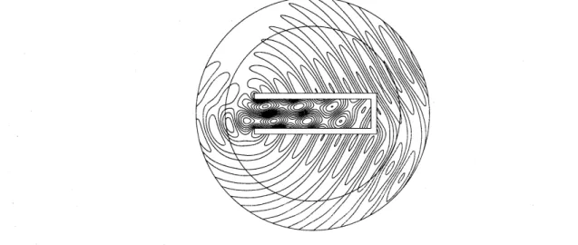
above. In

Figure 3, we display the contour lines of the real part of the numerical solutions in the

cases when $a=3\lambda$ and when $a=4\lambda$. Figure 3 shows good coincidenceofthose numerical

solutions, and suggests that ifwe

use our

ABC, we can get accurate numerical solutions

without enlarging radius of the artificial boundary.

5

Acknowledgments

The author would like to thank Professor Takashi Kako for introducing the controllability

method to him, Professor Teruo Ushijima for advising him to prove the uniqueness for the

semi-discrete solution, and Mr. Yoshio Tsukuda for giving himasoftwarefortriangulation,

Figure 2: Contour lines of the real part of the exact solution and of the real part of the

numerical solution obtained by using our ABC (2).

Figure 3: Contour lines of the real part of the numerical solutions in the cases when

$a–3\lambda$ and when $a=4\lambda$.

References

[1] C. Bardos and J. Rauch. Variational algorithms for the helmholtz equation using time

evolution and artificial boundaries. Asymptotic Analysis, 9:101-117, 1994.

[2] M. O. Bristeau, R. Glowinski, and J. P\’eriaux. _{Controllability methods for the}

com-putation of time-periodic solutions; application to scattering. J. Comput. Phys.,

$147(2):265-292$, 1998.

[3] M. J. Grote and J. B. Keller. On nonreflecting boundary conditions. J. Comput.