SINGULARITIES FOR VISCOSITY SOLUTIONS OF HAMILTON-JACOBI EQUATINS(Nonlinear Evolutions Equations and Their Applications)

SINGULARITIES

FOR VISCOSITY

SOLUTIONS

OF

HAMILTON-JACOBI

EQUATIONS

SHYUICHI

IZUMIYA1

AND GEORGIOS T.

KOSSIORIS2

1. INTRODUCTION

In this note we study the generation and propagation ofsingularities (shock waves) of the

solution of the Cauchy problem for Hamilton-Jacobi equations

(P) $\{$

$\frac{\partial y}{\partial t}+H(t, x_{1,\ldots,n}x, \frac{\partial y}{\partial x_{1}}, \ldots, \frac{\partial y}{\partial x_{n}})=0$

$y(\mathrm{o}, x_{1}, \ldots, x_{n})=\emptyset(_{X}1, \ldots, x_{n})$,

where $H$ and $\phi$ are $C^{\infty}$-functions.

Hamilton-Jacobi equations play an important role in various fields

e.g.,

calculus of

varia-tions (see e.g., [21]), optimal control theory (see e.g., [9]) and differential games (see e.g., [8]

and references cited therein).

For small time $t$ the solution of $(P)$ is classically determined using the characteristic

method. The geometric solution$y$ of (P) has been defined in ([13], [14]) in the framework of

one-parameterLegendrian unfoldings and it is constructed by the method of characteristics.

Although$y$ is initially smooth there is ingeneral a critical time beyond which characteristics

cross. The geometric solution past the critical time is multi-valued, that is singularities appear. The classification of singularities of $y$ has been studied in [13] (see also [15]) In

Section 2 we give a survey on the geometric framework $([13],[151,[16])$

.

The theoryof viscosity solutions (see [5]) has provided the right weak setting for thestudy

of (P). Existence and uniqueness of the solution of (P) in the viscosity

sense

have been established in [6]. The

single-valued

viscosity solution is continuous and coincides with the

smooth geometric solution until the first critical time. After the characteristics cross, the

viscosity solution develops shock waves i.e., curves across which the gradient of the viscosity

solution is discontinuous. The shock surfaces are referred to as singular

_surfaces

in the

literature of optimal control and differential games (see e.g., [3], [12]).

The method of constructing the weak solution byselecting theproper single-valued branch

was introduced by Tsuji $([_{-}^{;}2], [23])$ for Hamilton-Jacobi equations. Nakane in [20] has

con-structed the weak semi-concave solution past the first critical time in case that $H$ is convex

with respect to $\nabla y=$ $( \frac{\partial_{\mathrm{V}}}{\partial x_{1}}, \cdots , \frac{\partial y}{\partial x_{n}})$

.

The case of scalar conservation laws in $\mathbb{R}^{n}$ past the

first critical time has been studied by Nakane in [19]. In [4] Bogaevskii has shown that the

1Department of Mathematics, Faculty of Science, Hokkaido University, Sapporo 060, Japan

potential solution of the Burgers system with vanishing viscosity is given by the minimum

function of a certain family of smooth functions and given a classification for $n=1,2,3$. It

corresponds to the viscosity solution of the Hamilton-Jacobi equation when the Hamiltonian

is given by $H(p_{1}, \ldots p_{n})=\frac{1}{2}p_{1}^{2}+\cdots+\frac{1}{9,\sim}p_{n}^{2}$.

The viscosity solution of(P)for$\circ\sigma \mathrm{e}\mathrm{n}\mathrm{e}\mathrm{r}\mathrm{a}\mathrm{l}$ Hamiltonian in aneighborhood ofthe first critical

time has been constructed in [18] (see also [17], [20]) by selecting a continuous single-valued

branchof the graph of the geometric solution. Inwhich the shock curves of the weaksolution

corresponds to the intersection of the branches of the graph of the multi-valued geometric

solution. In order to study the evolution of the shock curves we follow the evolution of the

intersections of the branches defining the shock. After that we solve local Riemann problems

for each stage.

Here, we give proofs for some of the results. Further discussions will appear in elsewhere.

All maps considered here

a.re

class $C^{\infty}$ unless stated otherwise.

2. $\mathrm{G}\mathrm{E}\mathrm{O}_{1}\backslash 1\mathrm{E}\mathrm{T}\mathrm{R}\mathrm{I}\mathrm{c}$ SOLUTIONS

In this section we give a survey on the geometric framework and present the necessary

notations which was described in $([13],[15],[16])$.

Let $J^{1}(\mathbb{R}^{n}, \mathbb{R})$ be the 1-jet bundle of functions of $n$-variables which may be considered

as $\mathbb{R}^{2n+1}$ with a natural coordinate system _{$(x_{1}, \ldots , x_{n}, y,p_{1}, \ldots,p_{n})$}, where $(x_{1}, \ldots , x_{n})$ is a

coordinate system of $\mathbb{R}^{n}$. We also have a natural projection $\pi$ : $J^{1}(\mathbb{R}^{n}, \mathbb{R})arrow \mathbb{R}^{n}\cross \mathbb{R}$ given

by $\pi(x, y,p)=(x, y)$.

An immersion germ $i$ : $(L_{0}, u_{0})arrow J^{1}(\mathbb{R}^{n}, \mathbb{R})$ is said to be a Legendrian immersion germ

(i.e., Legendrian submanifold germ) if $\dim L=n$ _and $i^{*}\theta=0$, where $\theta=dy-\sum_{i=}^{n}1pidXi$.

The image of $\pi \mathrm{o}i$ is called the wave

front

set of $i$ and it is denoted by $W(i)$. We also

consider the 1-jet bundle $J^{1}(\mathbb{R}\cross \mathbb{R}^{n}, \mathbb{R})$ and the canonical 1-form $0$ on that space. Let

$(t, x_{1}, \ldots , x_{n})$ be a canonical coordinate system on $\mathbb{R}\cross \mathbb{R}^{n}$ and _{$(i, x_{1}, \ldots, x_{n}, y, S,p_{1}, \ldots,p_{n})$}

the corresponding coordinate system on $J^{1}(\mathbb{R}\cross \mathbb{R}^{n}, \mathbb{R})$. Then, the canonical 1-form is given

$\mathrm{b}\mathrm{y}\ominus=dy-\sum_{i1}^{n}=p_{ii}$. $dx-s\cdot dt=\theta-s\cdot di$.

We define the natural projection II : $J^{1}(\mathbb{R}\cross \mathbb{R}^{n}, \mathbb{R})arrow(\mathbb{R}\cross \mathbb{R}^{n})\cross \mathbb{R}$ by $\coprod(t, x, y, s,p)=$

$(t, x, y)$. We call the above 1-jet bundle an

unfolded

1-jet bundle.

A Hamilton-Jacobi equationis defined to be a hypersurface

(G-H-J) $E(H)=\{(t, x, y, s,p)\in J^{1}(\mathbb{R}\cross \mathbb{R}^{n}, \mathbb{R})|s+H(t, x,p)=0\}$

in $J^{1}(\mathbb{R}\cross \mathbb{R}^{n}, \mathbb{R}).$ A geometric (multi-valued) solution of $E(H)$ is a Legendrian

submanifold

$L$ in $J^{1}(\mathbb{R}\cross \mathbb{R}^{n}, \mathbb{R})$ lying in $E(H)$. In this case the wave front set $W(i)$ is “the graph” of the

geometric solution which is generally a hypersurface with singularities.

In order to study (P) we need the following framework: For any $c\in(\mathbb{R}, 0)$, we define

$E(H)_{\mathrm{C}}=\{(_{C}, X, y, -H(C, x,p),p)|(x, y,p)\in J1(\mathbb{R}n, \mathbb{R})\}$

.

Then, $E(H)_{\mathrm{c}}$ is a$(2n+1)$

-dimensional

submanifoldof$J^{1}(\mathbb{R}\cross \mathbb{R}^{n}, \mathbb{R})$ $\mathrm{a}\mathrm{n}\mathrm{d}\ominus_{\mathrm{c}}=|E(H)c=$

$E(H)_{c}$ by $\iota_{\mathrm{c}}(x, y,p)=(c, x, y, -H(C, X,p),p)$

.

The mapping $i_{c}$ is a contact diffeomorphism

and the following diagram is

commutative:

$J^{1}(\mathbb{R}^{n},\mathbb{R})\mathbb{R}^{n}\cross \mathbb{R}\pi\downarrow--\underline{\iota_{\mathrm{c}}}\mathbb{R}^{n}\cross \mathbb{R}E(H)\downarrow\pi_{\mathrm{C}}\mathrm{c}$

.

We say that a geometric Cauchy problem (with initial condition $L’$) associated with the

time parameter$(GcPT)$ is given

for

an equation $E(H)$ if there is given an n-dimensional

submanifold $i$ : _{$L’\subset E(H)$} with $i^{*}\ominus=0$ and $i(L’)\subset E(H)_{\mathrm{c}}$ for some $c\in(\mathbb{R}, 0)$. Since

$X_{H}\not\in TE(H)_{c}$, we have $X_{H}\not\in TL’$, where $X_{H}$ is the characteristic vector field given by

$X_{H}= \frac{\partial}{\partial t}+\sum_{=i1}n\frac{\partial H}{\partial p_{i}}\frac{\partial}{\partial x_{i}}+(\sum_{=i}n1p_{i}\frac{\partial H}{\partial p_{i}}-H)\frac{\partial}{\partial\tau/}-\frac{\partial H}{\partial t}\frac{\partial}{\partial s}-\sum_{1i=}\frac{\partial H}{\partial x_{i}}\frac{\partial}{\partial p_{i}}n$.

Byusing theclassical characteristic method, we canshow that thereexists aunique

geometric

solutions around $L’$.

We remark that Cauchy problem (P) is a GCPT. The initial submanifold is given by

$L_{\phi,0}=\{(0,$$x,$$\phi(_{X),H}-(0, x, \frac{\partial\phi}{\partial x}), \frac{\partial\phi}{\partial x})|x\in \mathbb{R}^{n\}}\subset E(H)_{0}$.

The problem of studying the singularities of the graph of the geometric solution is

formu-lated as follows:

Geometric Problem. Classify thegeneric bifurcati$ons$ ofwave fronts of

$\pi_{t}|$ : $L\mathrm{n}E(H)tarrow \mathbb{R}^{n}\cross \mathbb{R}$

with respect to the parameter $t$ (i.e., the

generic

bifurcations of wave fron$ts$ of

geometric

solutions along the $t\mathrm{i}me$ parameter).

Following [16], in order to study the singularities of the geometric solution weidentify

geo-metric solutions with one-parameterLegendrian unfoldings. Let $R$be an _$(n+1)$

-dimensional

smooth manifold, $\mu$ : $(R, u_{0})arrow(\mathbb{R},t_{0})$ be a submersion germ and

$\ell$ : $(R, u\mathrm{o})arrow J^{1}(\mathbb{R}^{n}, \mathbb{R})$ be

a smooth map germ. We say that the pair $(\mu, l)$ is a Legendrian family if $p_{t}=\ell|\mu^{-1}(t)$ is a

Legendrian immersion germ for any $t\in(\mathbb{R}, t_{0})$. Then we have the following simple but very

important lemma.

Lemma 2.1. Let $(\mu,\ell)$ be a $L\mathrm{e}_{\mathrm{o}}^{\sigma}endr\mathrm{i}\mathrm{a}\mathrm{n}$ family. Then there $eAst$ a uniq_$ue$ element $h\in$

$C_{u_{0}}^{\infty}(R)$ such that $f^{*}\theta=h\cdot d\mu$, where $C_{u_{0}}^{\infty}(R)$ is the $\mathrm{r}\mathrm{i}n_{\mathrm{o}}\sigma$ of$sm$ooth functiongerms at _{$u_{0}$}. Define a map

germ

$\mathcal{L}$ : $(R, u_{0})arrow J^{1}(\mathbb{R}\cross \mathbb{R}n, \mathbb{R})$ by

We can easily show that $\mathcal{L}$ is a Legendrian immersion germ. If we fix 1-forms $\ominus$ and $\theta$, the

Legendrian immersion germ $\mathcal{L}$ is uniquely determined by the Legendrian family

$(\mu,\ell)$. We

call $\mathcal{L}$ a Legendrian unfolding associated with the Legendrian family

$(\mu, \ell)$.

In order to study the evolutionoftheshock waves of theviscosity solutions of (P), we

have

to classify the generic types ofthe appearing $\sin\circ\cdot \mathrm{u}\mathrm{l}\mathrm{a}\mathrm{o}\mathrm{r}\mathrm{i}\mathrm{t}\mathrm{i}\mathrm{e}\mathrm{S}$i.e., how a singularity is generated,

how one type can change into another and how different types of $\sin\circ \mathrm{o}\mathrm{u}\mathrm{l}\mathrm{a}\mathrm{r}\mathrm{i}\mathrm{t}\mathrm{i}\mathrm{e}\mathrm{s}$ interact. We

study howvarious branches ofthemulti-valued$\circ\circ\cdot \mathrm{r}\mathrm{a}\mathrm{p}\mathrm{h}\nu V_{t}=(\{t\}\cross \mathbb{R}^{n}\cross \mathbb{R})\cap W(i)$

intersecting

at a point bifurcate in time for an arbitrary Hamiltonian $H(t, x,p)$ in [15]. We classify the

bifurcations of the branches of the $0\sigma \mathrm{r}\mathrm{a}\mathrm{p}\mathrm{h}$ by $\mathrm{c}\mathrm{l}\mathrm{a}\mathrm{S}\mathrm{S}\mathrm{i}\mathrm{f}\mathrm{y}\mathrm{i}\mathrm{n}_{\mathrm{o}}\sigma$ the

bifurcations

of singularities of

multi-Legendrian unfoldings which are expressed in terms of$\mathrm{m}\mathrm{u}\mathrm{l}\mathrm{t}\mathrm{i}- 0\sigma \mathrm{e}\mathrm{m}\mathrm{s}$.

Let $\mathcal{L}_{i}$

:

$(R, u_{0})arrow(J^{1}(\mathbb{R}\cross \mathbb{R}^{n}, \mathbb{R}),$_{$z_{i})(i=1, \ldots, r)$} be Legendrian unfoldings with

$\Pi(z_{i})=0$ where $z_{1},$_$\ldots,$$z_{r}$ are distinct. We call $(\mathcal{L}_{1}, \ldots, \mathcal{L}_{f})$ a multi-Legendrian

unfold-ing. Let $(\mathcal{L}_{1}, \ldots, \mathcal{L}_{r})$ and $(\mathcal{L}_{1}’, \ldots, \mathcal{L}_{r}’)$ be multi-Legendrian $\mathrm{u}\mathrm{n}\mathrm{f}\mathrm{o}\mathrm{l}\mathrm{d}\mathrm{i}\mathrm{n}_{\mathrm{o}}\sigma \mathrm{s}$. We say that these

are $P_{(r)}$-Legendrian equivalent if there exist contact diffeomorphism germs

$I\mathrm{i}_{i}’$ : $(J1(\mathbb{R}\cross \mathbb{R}n, \mathbb{R}),$ $z_{i})arrow(J^{1}(\mathbb{R}\mathrm{X}\mathbb{R}^{n}, \mathbb{R}),$ $Z_{i}’)$ $(i=1, , .., r)$

of the form $I1_{i}’(t, x, y, S,p)=(\phi_{1}(t), \phi 2(\iota, X, y), \phi 3(t, x, y), \phi^{i}4(t, X, y, s,p), \phi i\mathrm{s}(t, X, y, s,p))$ and

a diffeomorphism

germ

$\Psi$ : $(R, u_{0})arrow(R, u_{0}’)$ such that _{$I_{1_{i}}’\mathrm{o}\mathcal{L}_{i}=\mathcal{L}_{i}’0\Psi$} for any $i=$

$1,$$\ldots$ , $r$. It is clear that if two multi-Legendrian unfoldings are $P_{(r)}$-Legendrian equivalent,

then there exists a diffeomorphism$0\circ\cdot \mathrm{e}\mathrm{r}\mathrm{m}\Phi$ : $(\mathbb{R}\cross(\mathbb{R}^{n}\cross \mathbb{R}), 0)arrow(\mathbb{R}\mathrm{x}(\mathbb{R}^{n}\cross \mathbb{R}), 0)$ ofthe form

$\Phi(t, x, y)=(\phi_{1}(t), \phi_{2}(t, x, y), \phi_{3}(i, x,y))$ such that $\Phi(\bigcup_{i=1}^{\Gamma}W(\mathcal{L}_{i}))=\bigcup_{i=1}^{r}W(\mathcal{L}_{i})$. Thus the

above equivalence describeshow bifurcations ofwavefronts (i.e. graphs ofsolutions) interact.

We can define the notion of stability with respect to the $P_{(r)}$-Legendrian equivalence in

the same way as for the ordinary Legendrian stability (see $[1],[24]$_). Motivated by

Arnol’d-Zakalyukin’s theory $([1],[24])$, we can construct multi-generating families ofmulti-Legendrian

unfoldings and give a classification of$P_{(r)}$-Legendrian stable Legendrian unfoldings by using

the classification of multi-families of function germs in Zakalyukin [24]. We get a list of

classifications for $n=1,2,3$ in [15]. However, we only present the list of classifications for

$n=1$. For the case $n=2,3$, see [15].

Theorem 2.2 [15]. Suppose that $n=1$. Then a generic multi-Legendrian unfolding is

$P_{(r)}$-Legendrian $e\mathrm{q}$uivalent to

one

of the$mult\mathrm{i}- Le\sigma e\mathrm{n}\mathrm{O}dri\mathrm{a}\mathrm{n}$

unfoldings

in the following list :

$r=1$ ;

$0A_{1}$

:

$(t, u, \mathrm{O}, \mathrm{O}, \mathrm{o})$ ;

$0A_{2}$

:

$(t, 3u^{2},2u^{3}, \mathrm{o}, u)$ ;

$1A_{3}$

:

$(t, 4u^{3}+2ut, 3u^{4}+u^{-}’ t, -u^{2}, u)$.

$r=\underline{9}$ ;

$0(0A_{1}0A_{1})$

:

$((t, u, -u, \mathrm{o}, -1), (t,u, u, \mathrm{o}, 1))$ ;

1$(0A_{1}0A_{1})$

:

$((t, u, t\pm u^{2},1, \pm 2u), (t, u, 0,0,0))$ ;

$1A_{2}0A_{1}$ : $((t, 3u^{2}-t, 2u^{3}, u, u), (\mathrm{f}, u, -u, 0, -1))$.

$r=3$ ;

$0A_{1}0A_{1}0A1$

:

$((t, u,t-u, 1, -1), (t, u, \mathrm{O}, \mathrm{O}, \mathrm{o}), (t, u, u, \mathrm{o}, 1))$.

When we consider the geometric solution, we can get rid of the germ 1$(^{00}A_{11}A)$ from the

above list because the geometric solution is a $\mathrm{o}\mathrm{n}\mathrm{e}-\mathrm{t}_{0}$-one immersions into the unfolded l-jet

On

the otherhand, we have to

_identif.v

geometric

solutions withone-parameterLegendrian unfoldings in locally, so that we prove the followingrealization theorems.

Theorem 2.3 [13]. (1) The local solution of the GCPT for the Hamilton-Jacobi equation

$(G- H_{-}J)$ is a $Le_{\mathrm{o}}\sigma ex1$drian $\mathrm{u}\mathrm{n}fold\mathrm{i}\mathrm{n}_{\mathrm{o}}\sigma \mathcal{L}$ : $(\mathbb{R}\cross \mathbb{R}^{n}, \mathrm{o})arrow J^{1}(\mathbb{R}\mathrm{x}\mathbb{R}^{n}, \mathbb{R})$.

(2) Let $\mathcal{L}$ : $(\mathbb{R}\cross \mathbb{R}^{n}, 0)arrow J^{1}(\mathbb{R}\cross \mathbb{R}^{n}, \mathbb{R})$ be a $Le_{\mathrm{o}}\circ\cdot e\mathrm{n}$drian $\mathrm{u}\mathrm{n}foldi\mathrm{n}_{\mathrm{o}}\sigma$ associated with

$(\pi_{1},\ell)$. Then there exists a $C^{\infty}$-funciion _{$\circ\circ\cdot e\mathrm{r}mH(t, x_{1,\ldots,n}x,p_{1}, \ldots , p_{n})$} such that $\mathcal{L}$ is a local $s$olution of the$0\sigma e\mathrm{n}$eralized

$C\mathrm{a}$uchy problem associated with the $t\mathrm{i}me$parameter for the

Hamilton-Jacobi equation $(Garrow H- J)$, where th$\mathrm{e}$

$i\mathrm{n}\mathrm{i}$tial condiiion $is\circ\sigma \mathrm{j}\gamma en$ by _{$\ell(0, u)$}.

The above theorem$0\circ\cdot \mathrm{u}\mathrm{a}\mathrm{r}\mathrm{a}\mathrm{n}\mathrm{t}\mathrm{e}\mathrm{e}\mathrm{S}$that the class ofLegendrian unfoldings supplies the correct

class to describe the geometric solutions of (GCPT) for Hamilton-Jacobi equations. Thus,

generic results for the $\sin_{\mathrm{o}}\sigma \mathrm{u}\mathrm{l}\mathrm{a}\mathrm{r}\mathrm{i}\mathrm{t}\mathrm{i}\mathrm{e}\mathrm{s}$ of Legendrian $\mathrm{u}\mathrm{n}\mathrm{f}\mathrm{o}\mathrm{l}\mathrm{d}\mathrm{i}\mathrm{n}\circ\cdot \mathrm{s}\circ$ can be translated to $0\sigma \mathrm{e}\mathrm{n}\mathrm{e}\mathrm{r}\mathrm{i}\mathrm{c}$

results in the class of all Hamiltonians and all initial conditions. However, we have to also

concern ourselves with what are the types of singularities that the geometric solution to a

given Hamilton-Jacobi equation might exhibit. For the purpose, we need a kind of

non-degeneracy condition on the Hamiltonian function. We say that a Hamiltonian function

$H(t, x,p)$ is non-degenerate at $(t_{0}, x_{0,p_{0}})$ ifit $\frac{\partial^{2}H}{\partial p_{i}\partial_{Pi}}(t_{0}, x_{0},p\mathrm{o})\neq 0$ forsome $1\leq i,j\leq n$. This

condition is weaker than the condition that $H(t, x,p)$ is convex (or concave) with respect to

$(p_{1}, \ldots,p_{n})$-variables at $(t_{0}, x0,p_{0})$ for $n\geq 9arrow$. The foliowing theorem is a realization theorem

for generic $\sin_{\mathrm{o}}\sigma \mathrm{u}\mathrm{l}\mathrm{a}\mathrm{r}\mathrm{i}\mathrm{t}\mathrm{i}\mathrm{e}\mathrm{s}$ for agiven Hamilton-Jacobi equation.

Theorem 2.4 $([15],[16])$

.

Let $H(t, x,p)$ be a$\mathrm{n}on-de\mathrm{o}\sigma en$erate Hamiltonian function $0\sigma e\mathrm{r}m$ at

$(t_{0}, x_{0},p0)$ and $\mathcal{L}$ : $(R, u\mathrm{o})arrow(J^{1}(\mathbb{R}\cross \mathbb{R}^{n}, \mathbb{R}),$ $(t_{0}, x_{0}, y_{0}, S_{0}, p_{0}))$ be a $P_{(1)^{-Le}\circ}\sigma e\mathrm{n}$drian

stable

Legendrian unfoldi$n_{\mathrm{o}}\sigma$ associated with $(\mu, \ell)$. Then there exists a

$Le_{\mathrm{o}}\sigma endrianunfold\mathrm{i}\mathrm{n}_{\circ}\sigma \mathcal{L}$’

which is ageometric solntion of the Hamilton-Jaco$bi$ equation$s$

. $+H(t,.x,p)=0$ such that

$\mathcal{L}$

and $\mathcal{L}’$ are

$P_{(1)}-Le_{\circ}\sigma \mathrm{e}ndr\mathrm{i}\mathrm{a}n$ equivalen$t$.

We remark that $1A_{3}$ singularity (evenfor general $n$) describes how the singularity appears

fromasmooth solution. Theseare$P_{(1)0}-\mathrm{L}\mathrm{e}\sigma \mathrm{e}\mathrm{n}\mathrm{d}\mathrm{r}\mathrm{i}\mathrm{a}\mathrm{n}$stableLegendrianunfoldings, so that these

can be realized as geometric solutions at the non-degenerated point for a given

Hamilton-Jacobi equation. We can also specify the point at where the $1A_{3}$-singularity appears.

Theorem 2.5 [16]. If an $1A_{3^{-}}s\mathrm{i}n\sigma \mathrm{O}u.la\Gamma ity$ appears at $(t_{0}, x_{0,p_{0}})$, then $H(t, x,\mathrm{p})$ is

non-degenerate at $(t_{0}, x_{0,p_{0}})$

.

3. $\mathrm{v}_{\mathrm{I}\mathrm{s}\mathrm{c}\mathrm{o}}\mathrm{s}\mathrm{I}\mathrm{T}\mathrm{Y}$ SOLUTIONS

The viscosity solutions for nonlinear equations of first order have been introduced by

Crandall and Lions [6]. Such solutions need not be differentiable everywhere, as the only

regularity required in the definition is that of continuity. The function $y_{\mathfrak{v}}\in C(\mathcal{O})$ is a

viscosity solution of

(H-J) $\frac{\partial\tau/}{\partial t}+H(t, x, \frac{\partial y}{\partial x_{1}}, \ldots, \frac{\partial?/}{\partial x_{n}})=0$

in the open domain $\mathcal{O}\subset \mathbb{R}^{+}\cross \mathbb{R}^{n}$provided

for any $\psi\in C^{1}(\mathcal{O})$ for which $y_{\mathrm{U}}-\psi$ attains a local maximum (resp. local minimum) at the

point $(t, x)\in O$. The function $y_{\mathfrak{v}}\in C([0, \infty)\cross \mathbb{R}^{n})$ is a viscosity solution of the Cauchy

problem $(P)$ if and only ifit is a viscosity solution of (H-J) in the domain $(0, \infty)\cross \mathbb{R}^{n}$ and

satisfies the initial condition

$\lim_{tarrow 0+}y\mathfrak{o}(t, x)=\emptyset(_{X})$.

The above inequality $\mathrm{w}\mathrm{i}\mathrm{U}$ be referred as the viscosity criterion at the point $(t, x)$. We next

state the viscosity criterionin a form which is more usefulfor theconstruction of the solution.

To this end, assume that $\mathcal{O}\subset(0, \infty)\cross \mathbb{R}^{n}$ is open and that there is a smooth hypersurface

$\Gamma$ of $\mathbb{R}^{+}\cross \mathbb{R}^{\mathfrak{n}}$, which divides $\mathcal{O}$ into two open sets $O^{+}$ and $\mathcal{O}^{-},$ $\mathcal{O}=\Gamma\cup \mathcal{O}^{+}\cup \mathcal{O}^{-}$. Then we

have the following theorem.

Theorem 3.1. Let $y_{\mathfrak{v}}\in C(O)$ and $y_{\mathfrak{v}}=y_{\mathrm{t}\mathrm{l}}^{+}$ in $\mathcal{O}^{+}\cup\Gamma,$$y_{\mathfrak{v}}=y_{\mathrm{U}}^{-}$ in $O^{-}\cup\Gamma$ where

$y_{\mathrm{c}}^{\pm}\in$

$C^{1}(O^{\pm}\cup\Gamma)$. Then $y_{\mathrm{U}}$ is a viscosi$ty$ solution of (H-J) in

$\mathcal{O}$ if and on_$ly$ if the following conditions hold:

$a)y_{\mathrm{U}}^{+}$ and $y_{\mathfrak{o}}^{-}$ are $cl$assical $s$olutions of (H-J) in

$\mathcal{O}^{+}$ an

$d\mathcal{O}^{-_{r}}es_{\mathrm{P}^{e}}Ct\mathrm{i}_{\mathrm{V}}ely$,

\’o)

Ifthe vector$\tilde{\eta}=(H(i, x, \frac{\partial y^{+}}{\partial x})-H(t, X, \frac{\partial y^{+}}{\partial x}), -(\frac{\partial y^{+}}{\partial x_{\mathrm{t}}}-\frac{\partial\tau_{l^{-}}}{\partial x_{\mathrm{t}}}, ..., \frac{\partial_{J^{+}}}{\partial x_{n}},-\frac{\partial}{\partial}\iota_{-}^{-}xn))\mathrm{p}o\mathrm{i}\mathrm{n}ts$into

$\mathcal{O}^{+}$, then

$H(t,$$x,$$(1- \lambda)\frac{\partial y_{\mathfrak{d}}^{+}}{\partial x}+\lambda\frac{\partial y_{\mathfrak{v}}^{-}}{\partial x})-(1-\lambda)H(t, x, \frac{\partial y_{\mathrm{U}}^{+}}{\partial x})-\lambda H(t, x, \frac{\partial y_{\mathrm{c}}^{-}}{\partial x})\leq 0$ (resp. $\geq 0$),

where $\lambda\in[0,1]$

.

In pariicular, $the\circ\sigma r\mathrm{a}\mathrm{p}h$of$Hl\mathrm{i}$es respectively\’oelowor ab$o\mathrm{v}e$ the linesegment

$j_{\mathrm{o}in}in_{\mathrm{o}}\sigma$ the points $(H(t, X,)\partial x’\partial x)\underline{\partial}_{\mathrm{R}}y^{+}\underline{\partial}y\mathrm{R}^{+}$ and $(H(t, x, \frac{\partial?J^{-}}{\partial x}),\partial x)\underline{\partial}y\mathrm{B}^{-}$.

The proofof Theorem 3.1 is given in $([17],[18])$ as a direct application of Theorem 1.3 in

[7]. The conditionb) will bereferredin the sequelasthe viscosity criterion. The hypersurface

$\Gamma$ in the neighbourhood of which

$y_{0}$ has the properties specified in the above theorem is the

shock

_surface.

If the Hamiltonian is uniformly convex (or concave), we can automatically

construct viscosity solutions from

our normal

forms,

so

that

we can

easily draw the pictures

ofshock surfaces for lower

dimensional

cases. In [4] Bogaevskii has shown that the potential

solution of the Burgers system with vanishing viscosity is given by the minimum function of a

certain family of smooth functions. It corresponds to the viscosity solution of the

Hamilton-Jacobi equation when the Hamiltonian is given by $H(p_{1}, \ldots p_{n})=\frac{1}{2}p_{1}^{2}+\cdots+\frac{1}{2}p_{n}^{2}$. He has

drawn the pictures of shocks for this case. Our pictures are same as his pictures, so we do

not present these in here (see [4]).

On the other hand, Bogaevskii used Florin-Hopf-Cole method $([10],[11])$ to detect the

solution and it works only for the $\mathrm{B}\mathrm{u}\mathrm{r}_{\mathrm{o}}^{\sigma}\mathrm{e}\mathrm{r}\mathrm{S}$system. Here, we prove the analogous

statement

as the Bogaevskii’s assertion in the

case

when the Hamiltonian $H(p_{1}, \ldots,p_{n})$ is

convex

and

depends only onthe momentum. In thiscase we apply Bardi-Evans’ result [2] to oursituations

in stead of Florin-Hopf-Cole method. The geometric solution for (P) is given by

where

$\{$

$x(t, u)=u+t \frac{\partial H}{\partial p}(\frac{\partial\phi}{\partial x}(u)))$,

$p(t, u)= \frac{\partial\phi}{\partial x}(u)$

$y(t, u)=t \{-H(\frac{\partial\phi}{\partial x}(u\mathrm{I})+<\frac{\partial\phi}{\partial x}(u), \frac{\partial H}{\partial p}(\frac{\partial\phi}{\partial x}(u))>\}+\phi(u)$.

We consider a family of functions $F(t, x,p, q)=\phi(q)+<p,$

_{$(x-q)>-H(p)t$}

_{, where}

$(t, x,p, q)\in \mathbb{R}\cross \mathbb{R}^{n}\cross(\mathbb{R}^{n}\cross \mathbb{R}^{n})$ and $<,$$>\mathrm{i}\mathrm{s}$ the canonical inner product on $\mathbb{R}^{n}$

.

We have

$\Sigma(F)=\{(t, q+\frac{\partial H}{\partial p}(\frac{\partial\phi}{\partial q}(q))t, \frac{\partial\phi}{\partial q}(q), q)|(t, q)\in \mathbb{R}\cross \mathbb{R}n\}$ ,

where $\Sigma(F)$ is the set defined to be $\frac{\partial F}{\partial p:}=0$ and $\frac{\partial F}{\partial q_{i}}=0$. We now define amap $\Phi_{F}$

:

$\Sigma(F)arrow$

$J^{1}(\mathbb{R}\cross \mathbb{R}^{n}, \mathbb{R})$ by $\Phi_{F}(t, x,p, q)=(t, x, F.(t, x,p, q), \frac{\partial F}{\partial t}, \frac{\partial F}{\partial x})$. It follows that

$\Phi_{F}(t, q+\frac{\partial H}{\partial p}(\frac{\partial\phi}{\partial q}(q))t,$ $\frac{\partial\phi}{\partial q}(q),$$q)=$

$(t, q+ \frac{\partial H}{\partial p}(\frac{\partial\phi}{\partial q}(q))t,$ $-H( \frac{\partial\phi}{\partial q}(q))t+<\frac{\partial\phi}{\partial q}(q),$$\frac{\partial H}{\partial p}(\frac{\partial\phi}{\partial q}(q))>+\emptyset(q),$$-H( \frac{\partial\phi}{\partial q}(q)),$$\frac{\partial\phi}{\partial q}(q))$

.

This shows that the image of the map $\Phi_{F}$ is equal to $L_{\phi)t}$, namely, $F$ is a global generating

family of $L_{\phi,t}$

.

We refer the following result ofBardi-Evans [2].

Theorem 3.2. Assume that the Hamilton$ianH(p_{1}, \ldots , p_{n})$ is convex, then

$y(t, x) \equiv\inf \mathrm{s}\mathrm{u}\mathrm{p}qp\{\phi(q)+<p, (_{X}-q)>-H(p)t\}$

is the un$\mathrm{i}$que viscositysoluti

on

of(P).

Then we have the following theorem as a corollary of the above theorem.

Theorem 3.3. Assume that $H$ is uniformly convex and $\phi$ has the minimum. Let $L_{\phi,t}$ be

th$\mathrm{e}$geometric

$Solut\mathrm{i}\sim on(\mathrm{S})$ ofthe $\mathrm{c}au.Chy\mathrm{P}^{ro\mathrm{b}}l.em(\mathrm{P})$

.

Then

$y(t, x) \equiv\min_{y}\{y|(i, x, y)\in\Pi(L_{\phi,t})\}$

is the unique viscosi$ty$ solution of(P).

Proof.

Consider the family of functions $F(t, x,p, q)=\phi(q)+<p,$$(x$

.$-q)>-H(p)t$ . Since

$H(p)$ is uniformly convex, we have

where $\Sigma_{p}(F)=\{(t, x,p, q)|\frac{\partial F}{\partial p}.\cdot=x_{i}-q_{i}-\frac{\partial H}{\partial p}.\cdot(p)t=0i=1, \ldots, n\}$. It follows that

$\inf_{q}\sup_{p}\{\phi(q)+<p, (_{X-q})>-H(p)t\}=\inf_{q}\{F(t, q+\frac{\partial H}{\partial p}(p)t,p, q)\}$.

Since $\phi$ has the minimum

,

it is equal to

$\min_{q}\{F(t, q+\frac{\partial H}{\partial p}(p)t,p, q)\}=\min_{q}\{F(t, X,p, q)|(t, x,p, q)\in\Sigma_{p}(F)\}$.

On

the otherhand, we definefunctions $f_{i}(t, x,p, q)= \frac{\partial F}{\partial p_{i}}=X_{i}-q_{i}-\frac{\partial H}{\partial \mathrm{p}:}(p)t(i=1, \ldots , n)$

.

Since

$H(p)$ is uniformly convex, we have $\frac{\partial f_{1}}{\partial p_{i}}(t_{0,0,p0}x, q\mathrm{o})=-\frac{\partial^{2}H}{\partial p_{i}\partial pj}(p_{0})t_{0}\overline{\gamma}-\angle 0$, at any

point $(t_{0}, x_{0},p0, q0)$, so that there exist local smooth functions $g_{i}(t, x, q)(i=1, \ldots,n)$ near

$(t_{0}, x0,p_{0}, q_{0})$ such that $\Sigma_{p}(F)=\{p_{i}=g_{i}(t, x, q)\}$. Thus we have

$\frac{\partial F|\Sigma_{p}(F)}{\partial q_{i}}=\sum_{j}\frac{\partial F}{\partial p_{j}}(t, x, g(t, x, q), q)\frac{\partial g_{j}}{\partial q_{i}}(t, X, q)+\frac{\partial\phi}{\partial q_{i}}(q)-g_{i}(t, x, q)=\frac{\partial\phi}{\partial q_{i}}(q)-g_{i}(t, x, q)$ ,

so that $\Sigma(F)=\{(t, x,p, q)\in\Sigma_{p}(F)|\frac{\partial F|\Sigma_{\mathrm{n}}.(F)}{\partial q1}=0\}$. It follows that

$y(t, x) \equiv\min_{y}\{y|(t, x, y)\in\Pi(L_{\phi,\mathrm{t}})\}$

$= \min\{F(t, x,p, q)|(t, x,p, q)\in\Sigma(F)\}$

$(p,q)$

$= \min_{q}\{F(t, X,p, q)|(t, x,p, q)\in\Sigma_{p}(F)\}$

.

It is the unique viscosity solution for the Cauchy problem (P).

However, for general (non-convex) Hamiltonian, situations are quite different.

4. NoN CONVEX HAMILTONIANS IN ONE SPACE VARIABLE

In this section we stick to the Cauchy problen ofHamilton-Jacobi equation in one space

variable as follows:

(P) $\{$

$\frac{\partial y}{\partial t}+H(\frac{\partial?/}{\partial x})=0$

$y(0, x)=\phi(_{X)}$,

where $H$ and $\phi$ are $C^{\infty}$-functions. Since $H(p)$ is not assumed to be uniformly convex (or

concave), wecannot useTheorem 3.3, sothat the situations shouldbe quite complicated

even

for the one space variables $\mathrm{c}a\mathrm{s}\mathrm{e}$.

In this case the geometric solution is given by

where

$\{$

$x(t, u)=u+tH’(\phi’(u))$,

$p(t, u)=\phi’(u)$

$y(t, u)=t\{-H(\emptyset l(u))+\phi’(u)H’(\phi’(u))\}+\phi(u)$

.

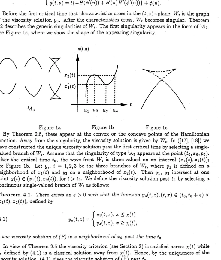
Before thefirst critical time that characteristics cross in the $(t, x)$-plane, $\nu V_{t}$ is the graph

of the viscosity solution $y_{\mathfrak{v}}$. After the characteristics cross, $\nu V_{t}$ becomes singular. Theorem

2.2 describes the generic singularities of$\nu V_{t}.$ Tlue first $\sin_{\mathrm{o}}\sigma \mathrm{u}\mathrm{l}\mathrm{a}\mathrm{r}\mathrm{i}\mathrm{t}\mathrm{y}$appears in the form of$1A_{3}$

.

See Figure la, where we show the shape of the appearing singularity.

x(t.u)

Figure la Figure lb Figure lc

By Theorem 2.5, these appear at the convex or the

concave

points of the Hamiltonian function. Away from the $\sin_{\mathrm{o}}\circ \mathrm{u}\mathrm{l}\mathrm{a}\mathrm{r}\mathrm{i}\mathrm{t}\mathrm{y}$, the viscosity solution is given by $W_{t}$. In ([17], [18]) we

have constructed the unique viscosity solution past thefirst criticaltime byselectinga

single-valuedbranch of$W_{t}$. Assume that thesingularityof type $1A_{3}$ appearsat the point $(t_{0}, x_{0,p_{0}})$

.

After the critical time $t_{0}$, the wave front $\mathrm{T}\prime V_{t}$ is three-valued on an interval $(x_{1}(t),$ $X_{2());}t$

see Figure $1\mathrm{b}$

.

Let

$y_{i},$ $i=1,2,3$ be the three branches of $\nu V_{t}$, where

$y_{1}$ is defined on a

neighborhood of $x_{1}(t)$ and $y_{2}$ on a $\mathrm{n}\mathrm{e}\mathrm{i}_{\mathrm{o}}\sigma \mathrm{h}\mathrm{b}\mathrm{o}\mathrm{r}\mathrm{h}_{0}\mathrm{o}\mathrm{d}$of $x_{2}(t)$

.

Then

$y_{1},$ $y_{2}$ intersect at one

point $\chi(t)\in(x_{1}(t), x_{2}(t))$, for $t>t_{0}$

.

We define the viscosity solution past $t_{0}$ by selecting a

continuous single-valued branch of $\nu V_{t}$ as follows:

Theorem 4.1. There exists an $\epsilon>0$ such that the function $y_{\mathfrak{v}}(t, x),$_{$(t, x)\in(t_{0}, t_{0}\backslash +\epsilon)\cross$}

$(x_{1}(t), x_{2}(t))$, defin$\mathrm{e}d$ by

(4.1) $y_{\mathfrak{v}}(t, x)=\{$

$y_{1}(t, x),$ $x\leq x(t)$

$y_{3}(t, x),$ $x\geq x(t)$,

is the viscosity solution of$(P)$ in a $\mathrm{n}e\mathrm{i}\circ h\mathrm{o}\mathrm{b}\mathrm{o}\mathrm{r}ho\mathrm{o}d$ of_{$x_{0}$} past the time$t_{0}$.

In view of Theorem 2.5 the

_Viscosit.v

criterion (see Section 3) is satisfied across $\chi(t)$ while

$y_{\mathfrak{v}}$ defined by (4.1) is a classical solution away from $\chi(t)$. Hence, by the uniqueness of the viscosity solution, (4.1) gives the viscosity solution of(P) past $i_{0}$.

By this construction,

we

have

extended

the viscosity solution beyond the first critical

time

$t_{0}$. Accordingto Theorem 2.5 the shock is generated in a convex or concave domains of$H(p)$,

so the viscosity criterion is automatically satisfied. The graph of the viscosity solution past

the first critical time is depicted by a full line in Figure $1\mathrm{c}$, where we

assume

that $H$ is

convex

in the neighborhood of the appearing singularity $1A_{3}$. The shock corresponds to the

intersection of the twobranches andit is called a genuine shock. The $\circ\sigma \mathrm{e}\mathrm{n}\mathrm{u}\mathrm{i}\mathrm{n}\mathrm{e}$ shock is defined

as the intersection of two incoming characteristics (or waves) and its speed is given by the

Rankine-Hugoniot condition

$\chi’(t)=\frac{H(_{J_{\mathrm{U}},\mathcal{I}}\tau^{+},(t,\chi(t)))-H(?^{-}/_{\mathfrak{o}},x(t,\prime\chi(t)))}{?J_{1})x+(t,x(t))-y^{-}\mathfrak{d},x(t,\chi(t))}$,

where $y_{\mathfrak{v},x}^{\pm}=\underline{\partial}_{A,\partial x^{-}}y^{\pm}$ and _{$\chi’(t)=\frac{d_{\mathrm{Y}}}{dt}(t)$}. Therefore in order to follow the evolution of the shock

we have to study the following questions:

a) How different branches of the multi-valued graph of $\nu V_{t}$ intersecting at one point

bifur-cate in time.

b) If the two branches initially defining the shock continue to cross, whether the viscosity

criterion is satisfied across the

intersection.

The normal forms of the generic bifurcations of different branches of $\mathrm{V}V_{\ell}$ are given in

Theorem 2.2. We depict these bifurcations in Figure 2.

1$(0A_{1}0A_{1})$

$0(0A_{1}0A_{1})$

$1A_{2^{0}}A_{1}$ $0A_{1}0A10A1$

If the viscosity criterion is satisfied at the time $t_{\alpha}=t_{0}+\epsilon$, we can choose the correct

branch of the graphs ofthe

geometric

solutions as viscosity solutions (see Figure 3).

$.-\Gamma^{\backslash }\backslash ^{-}\prime \mathrm{c}’\backslash$ $arrow-\backslash \wedge^{---}\backslash \backslash \prime\prime$ $arrow–\vee\wedge^{--}\backslash \prime 4$

$-\cdot-arrow_{--}.\vee--$ $arrow-\cdot \text{ノ_{}-\backslash }\vee--$

$’\backslash \mathrm{A}$ ’ ’ $\backslash$ ’

.

$\iota$ $\backslash$ ’ $\backslash$ $arrow$ $\nwarrow^{---},\prime \text{ノ}$ . $arrow$

$-\mathrm{Y}-\backslash \prime_{\backslash }’\backslash \backslash$

.

FIGURE 3

We willnow investigatehow the viscositycriterion canbe violatedacross theintersection of

two branches. Assume that a

generated

shock is defined by two intersecting branches $y^{-}$ and $y^{+}$

.

We denote by $\overline{y}$ (resp. $y^{+}$) the branch representing the viscosity solution for $x<\chi(t)$

(resp. $x>\chi(t)$). If the two branches remain intersected they evolve according to $0(_{-4_{1}}00A_{1})$

.

We denote by $\chi(t)$ the intersectionof the two branches. In the case when $H(p)$ has only

one

inflection point Kossioris [17] studied this problem and constructed the viscosity solutions.

We consider the general situation here. It is clear that for generic Hamiltonian function

$H(p),$ $H$ has only Morse type critical points and no tritangent lines.

So

we

assume

that the

Hamiltonian has the above properties. By Theorem 2.2, we have the following theorem.

Theorem 4.2. For a generic initi$\mathrm{a}l$ function $\phi$, if the viscosity criterion is violated at $t_{\alpha}$,

then the only following 8 cases may occu$\mathrm{r}$:

(1) The normal form is $0(^{0}A1A01)$ and$P^{\overline{+_{P^{-i}}}}\mathrm{S}ta\mathrm{n}^{\sigma}\circ ent$ to $the\circ\sigma r\mathrm{a}\mathrm{p}h$ of$H(p)$ at only one of

the points $P^{+},$ $P^{-}$ and the line is not $tan_{\mathrm{o}}\sigma ent$ to the $\mathrm{o}\mathrm{P}^{h}\sigma \mathrm{r}a$ at other points between these

$p_{\mathrm{o}\mathrm{i}n}tS$.

(2) The normal form is $0(^{0}A1A01)$ and $\overline{P^{+}P^{-}}\mathrm{i}_{S}$ not

$tan_{\mathrm{o}}\sigma ent$ to $the\circ\sigma \mathrm{r}aph$ of$H(p)$ at each

$p$oint $P^{+},$ $P^{-}$ and there exists on$l.v$ one another point between these points at where the

above lineis tangent to the$gr\mathrm{a}pl\iota$.

(3) The normal form is $0(^{0}A1A01)$ and $\overline{P^{+-_{\mathrm{i}\sigma}}P}stan\mathrm{e}nt\circ$ to thegraph of$H(p)$ at only one of

the points $P^{+},$ $P^{-}$ and there exists only on$\mathrm{e}$ another point between these points at where

the above line is $t$angent to the graph.

(4) The normal form is $0(^{0}A1A01)$ and$\overline{P^{+}P^{-}}\mathrm{i}_{S}$ tangent to the graph of_$H(p)$ at each point

of$P^{+},$ $P^{-}$.

(5) The normal form is $0(0A_{1}0A_{1})$ and $\overline{P^{+}P^{-}}\mathrm{i}_{S}$ not tangent to the graph of_$H(p)$ at each

point $P^{+},$ $P^{-}$ and there exists exactly trvo other points between these points at where the

above lineis $t$angent to thegraph.

(6) The normal $f\mathrm{o}\mathrm{m}$is $1A_{2}0A_{1}and\overline{P^{+}P-}is$ tangent to the graph of$H(p)$ at only one of the

$p$oints$P^{+},$ $P^{-}$ and thelineisnot tangent to thegraph at oiherpoints \’oetween these points.

(7) The norm$alfo\mathrm{m}$ is $0A_{1}0A_{1}0A1$ and$\overline{P^{+}P^{-\mathrm{j}_{S}}}tan_{\mathrm{o}}\sigma ent$ to the graph of$H(p)$ at only one

ofthe points $P^{+},$ $P^{-}$ and is not tangent to thegraph at other points between th_$ese$ points.

(8) The normal $fo\mathrm{m}$ is $0A_{1}0A_{1}0A_{1}$ and $\overline{P^{+}P-}\mathrm{i}s$ not $tan_{\mathrm{o}}\sigma \mathrm{e}nt$ to the graph of$H(p)$ at each

point $P^{+},$ $P^{-}$ and there exists only one another point between these points at where the

above line is tangen$t$ to the graph.

Here, $P^{+}=(y_{x}^{+}(t_{\alpha}, \chi(t\alpha)),$ $H(y^{+}x(t\alpha’\chi(t_{\alpha}))),$ $P^{-}=(y_{x}^{-(t_{\alpha}}, \chi(t\alpha)),$$H(yx-(t\alpha’\chi(t_{\alpha})))$ and

$\overline{P^{+}P^{-}}d\mathrm{e}notes$ the line through $P^{+},$$P^{-}$ in the $(p, H(p))$-plan$e$.

Proof.

By Theorem 2.2, we may

assume

that the first singularities appear in the form of$1A_{3}$.

After that the singularities of the graph of the geometric solution bifurcate in the forms of

$0(0A_{1}0A_{1}),$ $1(^{0}A_{1}0A_{1}),$ $1A_{2}0A_{1}$ or $0A_{1}0A_{1}0A1$. Since the characteristics in $J^{1}(\mathbb{R}\cross \mathbb{R}, \mathbb{R})$

never

cross, we can get rid of the case $1(0A_{1}0A_{1})$.

We already mentioned that the viscosity criterion is satisfiedpast the first critical time$t_{0}$,

so that it is satisfied until the time $t_{\alpha}$ when

$\overline{P^{+_{P^{-}}}}\mathrm{i}_{\mathrm{S}}$

tangent to the graph of $H(p)$. By the

assumptions on the Hamiltonian $H(p)$, we may consider the case that $\overline{P^{+}P^{-}}\mathrm{i}\mathrm{s}$ at most a

double tangent line for each normalform. We now distinguish each normal form. We denote

that $p^{+}=y_{x}^{+}(t_{\alpha}, \chi(t\alpha))=\phi’(u_{+})$ and $p^{-}=y_{x}^{-}(t_{\alpha}, \chi(t\alpha))=\phi’(u-)$

.

(A) $0(0A_{1}0A_{1})$: In this case each branch of the graph of geometric solution is a

Since the normal form $0(0A_{1}0A_{1})$ has trivial bifurcations along the time parameter, the

con-dition$y^{+}(t, \chi(t))=\overline{y}(t, \chi(t))$ defines a codimension $0$ submanifold in the corresponding jet

space, so that wemay ignore this condition. We

now

consider the following conditions

which

correspond to all possible cases:

(a) $\pm H’(\phi’(u_{+}))=,\frac{H(\emptyset\prime(u+))-H(\delta’(u-))}{\emptyset(u+)-\phi(u_{-)}},$, which defines a submanifold in $2J^{1}(\mathbb{R}, \mathbb{R})$ of

codi-mension 1.

Of

course, we have to consider the case that $\pm H’(\phi’(u_{-))}=,\frac{H(\phi’(u+))-H(\emptyset’(u-))}{\phi(u+)-\phi(u_{-})},$,

however this case is essentially contained in the above, so that we may ignore such

non-essentially different cases in the following arguments.

(b)There exists$u_{0}$with$u_{0}\neq u_{\pm}$ such$\mathrm{t}\mathrm{h}\mathrm{a}\mathrm{t}\pm H’(\phi’(u_{0}))=\frac{H(\phi’(u+))-H(\phi’(u-))}{\varphi’(u+)-\phi J(u_{-)}}$. This condition

defines a submanifold in $2J^{1}(\mathbb{R}, \mathbb{R})$ of codimension 1.

(c) There exists $u_{0}$ with $u_{0}\neq u\pm \mathrm{s}\mathrm{u}\mathrm{c}\mathrm{h}$that

$\pm H’(\phi’(u+))=\pm H’(\phi’(u_{0}))=\frac{H(\phi’(u_{+}))-H(\delta’(u_{-}))}{\phi’(u_{+})-\emptyset\prime(u_{-})}=\frac{H(\phi’(u_{+}))-H(\emptyset\prime(u\mathrm{o}))}{\phi’(u+)-\phi\prime(u\mathrm{o})}$

.

This condition defines a submanifold in $3J^{1}(\mathbb{R}, \mathbb{R})$ of codimension

3.

(d) $\pm H’(\phi’(u_{+}))=\pm H’(\phi’(u_{-))}=,\frac{H(\delta’(u+))-H(\phi\prime(u-))}{\phi(u+)-\phi(u_{-)}},$, which defines a submanifold in

$2J^{1}(\mathbb{R}, \mathbb{R})$ of codimension 2.

(e) There exist $u_{0},$ $u_{1}$ which are different from $u\pm \mathrm{s}\mathrm{u}\mathrm{c}\mathrm{h}$ that

$\pm H’(\phi’(u_{0}))=\pm H’(\phi’(u_{1}))=\frac{H(\phi’(u+))-H(\phi\prime(u_{-}))}{\phi’(u_{+})-\emptyset\prime(u_{-})}$

$= \frac{H(\phi’(u_{+}))-H(\emptyset\prime(u\mathrm{o}))}{\phi’(u_{+})-\phi’(u_{0})}=\frac{H(\phi’(u_{+}))-H(\emptyset\prime(u_{1}))}{\phi’(u_{+})-\phi^{l}(u_{1})}$

.

This conditiondefines a submanifold$\mathrm{o}\mathrm{f}_{4}J^{1}(\mathbb{R}, \mathbb{R})$ofcodimension4. Here, $rJ^{1}(\mathbb{R}, \mathbb{R})$isa

multi-1-jet space of functiongerm $\mathbb{R}arrow \mathbb{R}$. Eachsubmanifold in $rJ^{1}(\mathbb{R}, \mathbb{R})$ has at most codimension

$r$, so that we can not avoid such conditions by the multi-jet transversality theorem.

(B) $1A_{2^{0}}A_{1}$: In this

case

the normal form $1A_{2^{0}}A_{1}$ bifurcates at the time $t_{\alpha}$,

so

that

we

should consider the condition $y^{+}(t_{\alpha’\prime}\chi(t\alpha))=y^{-}(t_{\alpha}, \chi(t\alpha))$ for fixed $t_{\alpha}$

.

It defines a

subman-ifold in $2J^{1}(\mathbb{R}, \mathbb{R})$ of codimension 1. By the same arguments as the above, we can avoid the

conditions (c), (d) and (e). So we may consider the condition (a) or (b). We now show that

the condition (a) holds for the normal form $1A_{2}044_{1}$. On the $(t, x)$-plane, we denote $(t, \chi(t))$

the genuine shocks for $t\leq t_{\alpha}$. Suppose that the point $u$-corresponds to the cusp point at

the time $t_{\alpha}$. Then there exists a smooth function $u(t)$ such that $\chi(t)=u(t)+tH’(\phi’(u(t)))$

for $t\leq t_{\alpha}$ and $u(t_{\alpha})=u_{-}$, where we chooseoneof the branches of the graph of the geometric

solution corresponding to $u_{-}$

.

It follows that we have

$\chi’(t)=u’(t)(1+H’’(\phi’(u(t))\phi\prime\prime(t))+H’(\phi’(u(t))$.

Since the graph of the geometric solution has a singularity at $t_{\alpha}$, we have $\frac{\partial x}{\partial u}(t_{\alpha},$$u_{-)}=$

On

the other hand, by the Rankine-Hugoniot condition we have

$\chi’(t)=’\frac{H(y_{\emptyset}^{+}x(i,\chi(t)))-H(y^{-}\mathfrak{v},x(t,\chi(t)))}{y_{\mathfrak{v},x}^{+}(t,x(t))-y_{0}x-(t,\chi(t))},$

’

for $t\leq t_{\alpha}$.

Since

$\lim_{tarrow t_{\alpha}}y_{0x}^{\pm}(t,$_{$\chi)(t)))=\phi’(u\pm)$}, we have $\chi’(t_{\alpha})=\frac{H(\phi’(u+))-H(\phi’(u-))}{\varphi’(\mathrm{u}+)-\phi(u_{-})},$, so that we have $H’(\phi’(u_{-}))=\wedge^{-}H\phi’(u))H(\phi’(u-))$

.

This condition corresponds to the

case

(a)

$\phi’(\mathrm{u}+)-\phi’(u-)$

and we may get rid of the case (b).

(C) $0A_{1}0A_{11}0A$: In this

case

the normalformalso bifurcate at thepoint $t_{\alpha}$, sothat we can

get rid of the case (c), (d) and (e) by the similar reasons as those of the case (B). Since each

branch of the normal form is non-singular, the remaining two cases may occur in generic.

This completes the proof.

We can solve local Riemann problems and construct viscosity solutions for each case in

the above theorem. However, we only consider the cases (1) and (6) in this paper. We will

give the detailed considerations for all cases in elsewhere.

Case (1). We assume that the graph of the viscosity solution at the time $t\leq t_{\alpha}$ is depicted

as in Figure $4\mathrm{a}$

.

$\mathrm{H}(\mathrm{P})$

$H’(y_{x}^{-}(t \alpha’\chi(t\alpha)))=’\frac{H(y_{x}^{+}(t\alpha\chi(t\alpha)))-H(y_{x}^{-}(t\alpha x(t_{\alpha})))}{y_{x}^{+}(t_{\alpha},\chi(t\alpha))-y_{x}-(t\alpha’\chi(t\alpha))},=x’(t_{\alpha})$

.

We now distinguish two cases as follows:

a) If

for $t_{\alpha}\leq t<t_{\alpha}+\epsilon$ for sufficiently small $\epsilon>0$, then we can easily show that the viscosity

criterion is satisfied for $t<t_{\alpha}+\epsilon$

.

So

we can choose single valuedcontinuous branches of the

geometric solution as the viscosity solution.

b) If

$H’(y_{x}^{-((}t, xt)))< \frac{H(y_{x}^{+}(t,\chi(t)))-H(yx-(t,\chi(\iota)))}{y_{x}^{+}(t,\chi(t))-y\overline{x}(t,\chi(t))}$

for $t_{\alpha}\leq t<t_{\alpha}+\epsilon$ for sufficiently small $\epsilon>0$, then we can easily show that the viscosity

criterion is violated for $t_{\alpha}<t<t_{\alpha}+\epsilon$, so that a new way to build the solution is required

(cf., Figure 5).

$\mathrm{H}(\mathrm{D})$

$\mathrm{H}(\mathrm{P})$

FIGURE 5

In this case we can use the techniques in [12] to construct the contact discontinuity shock

curve and then obtain new characteristics. Lets consider the relation $H’(q)= \frac{H(p)-H(q)}{p-q}$

around $(q_{0},p\mathrm{o})$ with $q_{0}\neq p_{0},$ $H’(q_{0})= \frac{H(p_{0})-H(q_{0})}{p0-q0}$ and $H”(q_{0})\neq 0$

.

By the implicit function

theorem, thereexists a smooth function$\psi$ around$p_{0}$ suchthattheaboverelation isequivalent

to $q=\psi(p)$

.

We will first construct the contact discontinuity as the solution ofthe following

initial value problem.

$\{$

$x_{\mathrm{c}}’(t)=H’(\psi(yx(+t, x_{c}(t))))$,

$\chi_{\mathrm{C}}(t_{\alpha})=\chi(t\alpha)$

.

The characteristic which is started at a point $(\tau, \chi_{c}(\tau))$ should be satisfied the following:

$\{$

$x’(t)=H’(p(t))$,

$p’(t)=0$

$y^{l}(t)=-H(p(t))+p(t)H’(p(t))$,

with initial condition $x(\tau)=\chi_{c}(\tau),$ $y(\tau)=y^{+}(\tau, \chi_{c}(\tau))$ and $p(\tau)=\psi(y_{x}^{+}(\tau, \chi \mathrm{c}(\mathcal{T})))$. So the

solution is exactly given as follows:

$\{$

$\tilde{x}(t)=\chi \mathrm{c}(\mathcal{T})+(t-\mathcal{T})H;(\psi(y^{+}x(\mathcal{T}, xc(\mathcal{T}))\rangle)$,

$\tilde{p}(t)=\psi(y^{+}\mathcal{I}(\tau, \chi \mathrm{c}(\mathcal{T})))$

$\tilde{y}(t)=y^{+}(\tau, \chi_{\mathrm{C}}(\tau))$

By definition of the contact discontinuity, we have

$\chi_{\mathrm{C}}’’(t)=H’’(\psi(\phi(u_{+}(t))\frac{\partial\psi}{\partial p}(\phi’(u_{+}(t))\phi’’(u+(t))u_{+(}’t)$,

where $\chi_{c}(t)=u_{+}(t)+tH’(\phi(u_{+}(t)).$

Since

$\frac{\partial\psi}{\partial p}=,,\frac{H’(P)-H’(q)}{H(q)(p-q)}$

, we

have

$x_{c}’’(t)= \frac{H’(\phi\prime(u_{+}(t))-H\prime(\psi(\emptyset\prime(u+(t))))}{\emptyset^{l}(u_{+(t))-^{\psi(\phi’((t)))}}u+}\phi\prime l(u_{+}(t))u_{+}(\prime t)$ . We also have $\chi’(t)=u_{+}’(t)\{1+tH’’(\phi’(u+(t))\phi’’(u_{+}(t))\}+H’(\phi’(u_{+}(t)))$

.

It follows that $\chi_{\mathrm{c}}’’(t)=-,\frac{(H’(\emptyset\prime(u_{+}(t)))-H\prime(\psi(\phi’(u_{+}(t)))))2}{\emptyset(u_{+(t))-^{\psi(\phi((t)))}}u+},\frac{\phi’’(u_{+}(t))}{1+tH’\prime(\emptyset(u+(t))\phi’’(u_{+}(t))},\cdot$ Since

$\frac{\partial x}{\partial u}(t, u_{+}(t))=1+tH’’(\emptyset’(u_{+}(t)))\phi\prime\prime(u+(t))$,

we may assume that $1+tH”(\emptyset’(u_{+}(t)))\phi’’(u_{+}(t))>0$

.

So $\chi_{\mathrm{c}}(t)$ is convex if and only if

$\phi’’(u_{+}(t))>0$

.

We suppose that $\phi’’(u_{+}(t))\leq 0$ and denote $\chi_{c}(t)=u_{+}(t)+tH’(\phi(u+(t))=$

$u_{-}(t)+tH’(\phi(u_{-}(t)))$, where $u_{-}(t)$ (resp. $u_{+}(t)$) is the point corresponding to the charac-teristic from the right (resp. left) side of$(t, \chi_{\mathrm{c}}(t))$

.

We distinguish two cases as follows:

b-l) If $\phi’’(u_{-}(t))>0$, then $\phi’$ is monotone.

Since

$u_{-}’(t)<0,$ $\phi’(u_{-}(t))$ moves to the left

direction, so that the viscosity criterion is satisfied across $\chi$

.

$\mathrm{b}-2)\mathrm{I}\mathrm{f}\phi’’(u_{-}(t))<0$ and the viscosity criterion is violated across $\chi$ for $t>t_{\alpha}$, then 1+ $tH”(\emptyset’(u_{-}(t)))\emptyset\prime\prime(u_{-}(t))>0$near$t_{\alpha}$

.

Differentiatethe equality$\chi_{c}(t)=u_{-}(t)+tH’(\phi(u_{-}(t))$

with respect to $t$, then we have

$x’(t)-H’(\phi’(u-(t)))=\{1+tH’’(\emptyset’(u-(t)))\phi’’(u-(t))\}u_{-(}’t)$

.

Since

$x’(t)=, \frac{H(\phi’(u_{+}(t)))-H(\phi’(u_{-}(t)))}{\phi(u_{+}(t))-\phi\prime(u_{-}(t))}>H’(\phi’(u_{-}(t)))$, we have $u_{-}’(t)>0$, so that $u_{-}(t)$ is increase, which is a contradiction.

Hence, if the viscosity criterion is violated for $t>t_{\alpha}$, the contact discontinuity curve $\chi$ is

We draw the oicture which is $\mathrm{i}\mathrm{l}\mathrm{l}\mathrm{u}\mathrm{s}\mathrm{t}\mathrm{r}\mathrm{a}\mathrm{t}\mathrm{i}\mathrm{n}\not\subset$the situations

as

follows:

Case (6). The bifurcations of thegraphs ofthe geometric solution at the time $t_{\alpha}$ is depicted

as follows:

We use the

same

notation as the case (1).

Since

$u_{-}(t_{\alpha})$ corresponds to the cusp point,

we have $1+t_{\alpha}H’’(\phi(u_{-(t}\alpha)))\phi\prime\prime(u_{-}(t)\alpha)=0$. Let $(t, \sigma(t))$ be the locus of the cusps,

where

we denote $\sigma(t)=\sigma_{(}t)+tH’(\phi’(\sigma-(t)))$ as the family of

characteristics

come from the left

side, so that we have $1+tH”(\phi’(\sigma-(t)))\phi;’(\sigma_{-}(t))=0$ and $\sigma_{-}^{J}(t)<0$. It $\mathrm{f}\mathrm{o}\mathrm{U}\mathrm{o}\mathrm{w}\mathrm{s}$ that $H”(\phi’(\sigma-(t)))\phi’’(\sigma-(t))<0$ and $\sigma’(t)=H’(\phi’(\sigma’-(t))$.

Differentiating

the equation again,

we get $\sigma’’(t)=H’’(\emptyset^{l}(\sigma_{-}(t))\phi\prime\prime(\sigma-(t))\sigma_{-}^{;}(t)>0$. Therefore $(t, \sigma(t))$ is strictly

convex.

We denote $\chi(t)=u_{-}(t)+tH’(\phi’(u_{-}(t)))=u_{+}(i)+tH’(\phi’(u_{+}(t)))$ for $t\leq t_{\alpha}$, then we have $u_{-}(t_{\alpha})=\sigma_{-}(t_{\alpha})$, so that $\sigma’(t_{\alpha})=H’(\phi^{;}(\sigma_{-}(t\alpha)))=H’(\phi(u-(t_{\alpha})))=\chi’(t_{\alpha})$ by the proof of

Theorem 4.2. We also construct the contact discontinuity $(t,xc(\prime t))$ exactly the same as that

ofin the case (1). We need examine the following two subcases.

a) Assume that $\sigma(t)\geq\chi_{c}(t)$ for $t\geq t_{\alpha}$. Since both $\chi_{\mathrm{c}}$ and $\sigma$ are

convex

near $t_{\alpha}$, we have

that $\sigma’’(t_{\alpha})>\chi’’(t_{\alpha})$

.

On the other hand, we have

$y(t, \sigma_{\pm}(t))=t\{-H(\phi’(\sigma\pm(t)))+\phi’(\sigma\pm(t))H’(\phi’(\sigma_{\pm}(t)))\}+\phi(\sigma\pm(t))$,

$\frac{d\mathrm{c}/}{dt}(t, \sigma+(t))=-H(\phi’(\sigma+(t)))+\phi’(\sigma_{+}(\iota))H’(\emptyset’(\sigma_{+}(t)))$

$+\phi’(\sigma_{+}(t))\sigma’(+t)\{1+tH^{l}’(\phi’(\sigma_{+}(t)))\phi\prime\prime(\sigma+(t))\}$

and

$\frac{dy}{dt}(i, \sigma_{-}(t))=-H(\phi’(\sigma_{-}(t)))+\phi’(\sigma_{-}(t))H’(\phi’(\sigma_{-(}t)))$. Let $A(t)=y(t, \sigma+(t))-y(t, \sigma_{-(t)})$ for $t\geq t_{\alpha}$.

Differentiating the equality $\sigma_{-}(t)+tH’(\phi’(\sigma_{-(}t)))=\sigma_{+}(t)+tH’(\phi’(\sigma+(t)))$ with respect

to $t$, we get $\sigma_{+}’(t)\{1+tH’’(\phi’(\sigma_{+}(t)))\emptyset l’(\sigma+(t))\}=H’(\phi’(\sigma_{-}(t)))-H’(\phi’(\sigma+(t)))$

.

It follows that $A’(t)=H’(\emptyset(\sigma_{-}(t)))\{\phi’(\sigma+(t))-\phi l(\sigma-(t))\}-(H(\phi’(\sigma_{+}(t)))-H(\phi^{;}(\sigma_{-}(t))))$ . Furthermore, we have $A”(t)=(H’(\phi’(\sigma_{-}(t))-H’(\phi’(\sigma+(t)))\phi^{;\prime}(\sigma_{+}(t))\sigma_{+(t)}’$ $+H”(\phi;(\sigma_{-}(t)))\phi’’(\sigma-(t))\mathrm{t}\phi’(\sigma+(t))-\phi;(\sigma_{-}(t))\}\sigma_{-()}\prime t$

.

Since $\sigma_{+}’(t)=,,,\frac{H’(\phi’(\sigma-(t))-H’(\phi’(\sigma+(t))}{1+tH(\phi(\sigma+(t))\varphi(\sigma+(t))},$, and _{$\sigma’’(t)=H’’(\phi’(\sigma-(t)))\phi’’(\sigma-(t))\sigma_{-}’(t)$}, we have

$A”(t)=, \frac{(H’(\phi’(\sigma-(t))-H\prime(\phi’(\sigma_{+}(t)))}{1+tH’(\emptyset(\sigma+(t))\emptyset(\sigma_{+}(t))},,,\underline’\phi\prime\prime(\sigma+(t))+\sigma(\prime\prime t)\{\phi’(\sigma+(t))-\phi’(\sigma-(t))\}$ .

On

the other hand, as we already calculated in the case (1) that

At the point $t=t_{\alpha}$, we have $u\pm(t_{\alpha})=\sigma\pm(t_{\alpha})$ and $\psi(\phi’(\sigma_{+}(t_{\alpha})))=\phi’(\sigma_{-}(t\alpha))$, so that

$\chi_{c}’’(t_{\alpha})=-,\frac{(H’(\emptyset\prime(u_{+}(t\alpha))-H’(\psi(\phi\prime(u+(t_{\alpha})))))^{2}}{\phi(u_{+}(t_{\alpha}))-\psi(\phi(u_{+}(t_{\alpha})))},,\cdot$

Thus, we have

$A”(t_{\alpha})=(\sigma’’(t\alpha)-x_{\mathrm{c}}’’(t_{a}lpha))(\phi’(\sigma+(t\alpha)-\phi’(\sigma_{-}(t\alpha))$

.

Since $\sigma’’(t_{\alpha})>\chi_{c}’’(t)\alpha$ and $\phi’(\sigma_{+}(t)\alpha<\phi’(\sigma_{-}(t_{\alpha})$, we have $A”(t_{\alpha})<0$

.

This

means

that $A’(t)<0$ near $t_{\alpha}$, so $y(t, \sigma_{+}(t))<y(t, \sigma_{-}(t))$.

We also consider

$y_{+}(t)=t\{-H(\phi’(u+(i)))+\phi’(u_{+}(t))H’(\phi’(u_{+}(t)))\}+\phi(u_{+}(t))$

and

$y_{\alpha}(t)=t\{-H(\phi’(u_{\alpha}))+\phi’(u\alpha)H’(\emptyset^{l}(u\alpha))\}+\phi(u_{\alpha})$,

where $u_{\alpha}=\sigma_{-}(t_{\alpha})$ and $x(t, u_{\alpha})=u_{\alpha}+\iota H’(\emptyset’(u_{\alpha}))=x(t, u_{+}(t))=u_{+}(t)+tH’(\phi’(u_{+}(t)))$

.

Differentiating the last equality, we get

$H’(\emptyset’(u_{\alpha}))=u_{+}’(t)+H’(\phi’(u_{+}(t)))+tH’’(\phi^{l}(u_{+}(t)))\phi’’(u+(t))u_{+}(\prime t)$

.

Then $y_{+}’(t)=-H(\phi’(u_{+(t)})+\phi’(u_{+}(t))H’(\emptyset’(u_{+}(t)))$ $+tH”(\phi’(u_{+}(t)))\phi’(u_{+}(t))\phi’’(u+(t))u_{+(t)}^{l}+\phi’(u_{+}(t))u_{+}’(t)$ $=-H(\phi’(u_{+}(t)))+\phi’(u_{+}(t))H’(\emptyset’(u_{+}(t)))$

.

So we obtain $\frac{d}{dt}(y_{\alpha}(t)-y_{+}(t))=H(\phi’(u_{+}(t)))-H(\phi’(u_{\alpha}))-H’(\phi’(u_{\alpha}))(\phi’(u_{+}(t))-\phi’(u_{\alpha}))$

.

Since $\phi’(u_{+}(t))<\phi’(u_{\alpha})$ and $\phi’(u_{\alpha})$ is in the

convex

region of$H(p)$, we have

$H’( \phi’(u_{\alpha}))<,\frac{H(\phi’(u_{+}(t)))-H(\emptyset\prime(u\alpha))}{\phi(u_{+}(t))-\phi\prime(u_{\alpha})}$,

so that we have $\frac{d}{dt}(y_{\alpha}(t)-y_{+}(t))<0$. This means that $y_{\alpha}(t)<y_{+}(t)$ for $t>t_{\alpha}$

.

Thesesituation describesthat the two branches of the multi-valued graph haveintersection

for $t>t-\alpha$

.

This contradicts to the assumption that the singularity is 1

b) Here we assume that $\sigma(t)<\chi_{c}(t)$ for $t>t_{\alpha}$. In this subcase two shocks bifurcates from

See

Figure

9.

FIGURE 9

The left one is a new shock given $\mathrm{b}.\mathrm{v}$ the intersection of the original characteristic from

the left side and the new characteristic from the contact discontinuity (i.e., the

_rarefaction

waves).

By definition, wehave

$\tilde{y}_{\alpha}(t)=(t-t\alpha)\{-H(\psi(yx+(t\alpha’\chi_{\mathrm{C}}(t_{\alpha}))))+\psi(yx(+tx\alpha’ \mathrm{c}(tlpaha)))H\prime\prime(\psi(y_{x}^{+}(t\chi_{\mathrm{c}}(\alpha’ t_{\alpha}))))\}$

$+y^{+}(t_{\alpha},x(t\alpha))$

and

$y-(t)=t\{-H(\phi’(u_{-}(t)))+\emptyset^{l}(u_{-(t))H^{;}(\emptyset(u}\mathrm{t}t)))\}+\phi(u_{(}t))$,

where $u_{\alpha}+tH’(\emptyset’(ualpha)))=x(t,u_{-}(t))=u_{-}(t)+iH’(\phi’(t))$

.

Differentiatingthe last equality, we get

$u’-(t)+H’(\emptyset’(u_{-}(t)))+tH’’(\emptyset’(u_{-}(t)))\phi\prime\prime(u-(t))u\mathrm{L}(t)=H’(\phi^{l}(u\alpha))$

.

Then

$y_{-}’(t)=-H(\phi’(u_{-}(t)))+\phi’(u_{-}(t))H’(\phi(u(t)))$

$+tH”(\emptyset l(u_{-}(t)))\phi r(u_{(}t))\phi’’(u_{-}(t))u\mathrm{L}(t)+\phi’(u_{-}(t))u_{-}^{;}(t)$

$=-H(\phi’(u_{-}(t)))+\phi’(u-(t))H’(\phi(u\alpha)$

So

we obtain

Since

$u_{-}(t)<u_{\alpha}$ and both of $\phi’(u_{(}t)),$ $\phi’(u_{\alpha})$

are

in the

convex

region of $H(p)$,

we have

$\phi’(u_{(}t))>\phi’(u_{\alpha}))$ and

$H’( \phi’(u_{\alpha}))>\frac{H(\phi’(u-(t))-H(\phi’(u_{\alpha}))}{\emptyset^{J}(u_{-}(t))-\phi\prime(u_{\alpha})}$,

so that we obtain $\frac{d}{dt}(\tilde{y}_{\alpha}(t)-y_{-}(t))<0$. Since $\tilde{y}_{\alpha}(t_{\alpha})=y_{-}(t_{\alpha})$, the last inequ&ity means

that $\tilde{y}_{\alpha}(t)<y_{-}(t)$ for $t>t_{\alpha}$

.

We also consider

$\tilde{y}_{\alpha}(t, \sigma(i))=(t-\mathcal{T}(t))\{-H(\psi(y_{x}(+\mathcal{T}(t), x_{c}(\tau(t))))$

$+\psi(y_{x}^{+}(T(t), \chi c(\mathcal{T}(t))))H’’(\psi(y^{+}x(\mathcal{T}(t), \chi_{\mathrm{c}}(\mathcal{T}(t)))))\}$

$+y_{x}^{+}(\mathcal{T}(t), \chi c(\mathcal{T}(t)))$

and

$y-(t, \sigma(t))=t\mathrm{t}-H(\phi’(\sigma_{-}(t)))+\phi’(\sigma_{-}(t))H’(\phi(\sigma_{-}(t))\}+\emptyset(\sigma-(t))$,

where

$y^{+}(\tau(t), \chi \mathrm{C}(\mathcal{T}(t)))=T(t)\mathrm{t}-H(\emptyset’(\tau(t)))+\emptyset’(\mathcal{T}(t))H’(\phi(\tau(t))\}+\phi(\mathcal{T}(t))$,

$y_{x}^{+}(\tau(t), \chi_{\mathrm{c}}(\tau(t)))=\emptyset^{l}(u_{+(\tau}(t)))$

and

$\sigma(t)=\sigma_{-}(t))+tH’(\phi’(\sigma_{-}(t))=\chi_{C}(\mathcal{T}(t))+(t-\mathcal{T}(t))H’(\psi(\phi’(u_{+}(t)))$

.

Since $\chi_{\mathrm{c}}(\tau)=H’(\psi(\phi’(u_{+}(\tau)))$ and $1+tH”(\emptyset’(\sigma_{-}(t)))\phi’’(\sigma_{-}(t))=0$, differentiating the above equality, we get

$H’(\phi’(\sigma_{-}(t)))=H’(\psi(\phi’(u+(\mathcal{T}(t))))$

$+(t-T(t))H”( \psi(\phi(u+(\mathcal{T}(t))))\frac{d\psi}{dp}\emptyset’(u+(\mathcal{T}(t)))u_{+(\mathcal{T}(t))}’\tau’(t)$

.

Then

$\tilde{y}’(t, \sigma(t))=\tau l(t)\{-H(\emptyset’(u_{+}(_{\mathcal{T}(}t))))+\phi’(u+(\mathcal{T}(t)))H’(\phi’(u_{+}(\tau(t))))\}$

$+\tau(t)\phi’(u_{+^{\tau}}(t))H\prime\prime(\phi’(u_{+}(\tau(t))))\phi’’(u+(\tau(t)))u_{+(}’\tau(t))\mathcal{T}’(t)$ $+\phi’(u_{+}(\mathcal{T}(t)))u(’+\mathcal{T}(t))\mathcal{T}’(t)$ $+(1-\mathcal{T}’(t))\{-H(\psi(\phi’(u+(\mathcal{T}(t)))))+^{\psi(\emptyset(}\prime u+(\mathcal{T}(t)))H’(\psi(\emptyset’(u+(\tau(t)))))\}$ $+(t- \mathcal{T}(t))\psi(\emptyset’(u_{+}(\tau(t))))H\prime\prime(\psi(\phi’(u+(\mathcal{T}(t)))))\frac{d\psi}{dp}\phi’’(u_{+}(\tau(t)))\mathcal{T}’(t)$ $=\mathcal{T}’(t)\{H(\psi(\emptyset;(u_{+}(\tau(t)))))-H(\phi’(u_{+}(\tau(t))))$ $+(\phi’(u_{+}(\tau(t)))-\psi(\phi’(u_{+}(\tau(t))))H’(\psi(\emptyset l(u_{+}(\tau(t)))))\}$ $+\psi(\phi^{l}(u_{+(\tau(}\iota))))H’(\phi’(\sigma_{-}(t))-H(\psi(\phi’(u_{+}(\tau(t)))))$

.

By definition, we have

$H’( \psi(\phi’(u+(\mathcal{T}(t)))=\frac{H(\phi\prime(u_{+}(\tau(t))))-H(\psi(\phi\prime(u_{+}(\tau(t)))))}{\phi’(u_{+}(\mathcal{T}(t)))-\psi(\phi’(u_{+}(\mathcal{T}(t))))}$,

so that

$\tilde{y}’(t, \sigma(t))=\psi(\phi’(u_{+}(\tau(t))))H’(\phi’(\sigma(t)))-H(\psi(\phi l(u_{+}(\tau(t))))$

.

Thus we have

$\frac{d}{dt}(\tilde{y}(t, \sigma(t))-y-(t, \sigma(t)))=H’(\phi’(\sigma_{(t)})-H(\psi(\phi’(u+(\tau(t))))$

$-H’(\phi’(\sigma(t)))(\phi;(\sigma_{-}(t))-\psi(\emptyset’(u+(\mathcal{T}(t)))))$

.

Since both $\phi’(\sigma_{-}(t))$ and $\psi(\phi’(u_{+((t}\mathcal{T}))))$ belong to the

concave

region of$H(p),$ $\emptyset’(\sigma-(t))<$

$\psi(\phi’(u+(\tau(t))))$ for $t>i_{\alpha}$

.

Therefore

$\frac{H’(\emptyset\prime(\sigma(t))-H(\psi(\phi;(u_{+}(\tau(t))))}{\phi’(\sigma_{-}(t))-\psi(\phi’(u_{+}(\tau(t))))}<H’(\phi’(\sigma(t)))$,

hence we have $\frac{d}{dt}(\tilde{y}(t, \sigma(t))-y-(t, \sigma(t)))>0$. Since $\tilde{y}(t_{\alpha}, \sigma(t\alpha))=y-(t_{\alpha}, \sigma(t\alpha))$, the above

inequality means that $\tilde{y}(t, \sigma(t))>y_{-}(t, \sigma(t)))$ for$t>t_{\alpha}$. It follows that, there exists aunique

$(t, \chi_{r}(t))$ with $x(t,u_{\alpha})<\chi_{r}(t)<\sigma(t)$, such that $\tilde{y}(t, \chi_{r}(t))=y-(t, x_{r}(t))$

.

Then we can draw the picture of the graph of the viscosity solution for $t>t_{\alpha}$ and the

bifurcation of the shock curves around $t_{\alpha}$. (cf., Figure 10)

FIGURE

10

For other cases, the detailed discussions will appear in elsewhere.

REFERENCES

1. V.I. Arnol’d, S. M. Gusein-Zade

_a.nd

A.N. Varchenko, Singularities _{ofDifferentiable} Maps, Birkhauser,

1986.

2. M. Bardi and L. C. Evans, On Hopf’s _{formulas for} solutions _ofhamilton-Jacobi equations, Nonlinear

Analysis 8 (1984), 1373-1389.

3. P. Bernhard, Singular _surfaces in

_differential

games, an introduction; in Differential Games and Appli-cations, Lecture Notes in Control and Information Sciences (P. Hagedorn et al., eds.), vol. 3, Springer

4. A. Bogaevskii, _{Modifications of}singularities _ofminimum _functions and $bifi_{lrc}ations$ ofshock waves at

the Burgers equation with vanishing viscosity, Leningrad Math. J. 1 (1990), 807-823.

5. M.G. Crandall,H. Ishii andP.-Lions, User’s guidetoviscositysolutions_ofsecond order partialdifferential

equations, Bull. Amer. Math. Soc. 27 (1992), 1-67.

6. M. G. CrandallandP.-Lions, Viscositysolutions of$Hamiu_{\mathit{0}}n$-Jacobi $equ\dot{a}$tions,Trans. Amer. Math. Soc.

277 (1983), 1-42.

7. M. G. Crandall, L.C. Evans and P.-L. Lions, Some properties _ofviscosity solutions _ofHamilton-Jacobi

equations, Trans.Amer. Math. Soc 282 (1984), 487-502.

8. L. C. Evans and P. E. $\mathrm{S}_{\mathrm{o}\mathrm{u}_{\mathrm{o}}\mathrm{a}\mathrm{n}}\sigma \mathrm{i}\mathrm{d}\mathrm{e}\mathrm{S}$,

Differential

games and representation formulas for solutions of

$Hami\iota_{t_{\mathit{0}}-Ja}n$cobi-Isaacs equations, Indiana Univ. Math. J. 33 (1984), 773-797.

9. W. H. Fleming and H. M. Soner, Controlled Markov Processes and $Vi_{Scos}ity.Solutions$, Springe.r-Verlag,

1993.

10. V. A. Florin, Some simplest nonlinear problems ofthe consolidation _of an aqueously saturated earthen

medium, Izv. Akad. Nauk SSSR Otdel.Tekhn. Nauk 9 (1948), 1389-1397.

11. E. Hopf, Generalized solution _ofnon-linear equations offirst order, Jour. of Math. and Mechanics 14

(1965), 951-973].

12. R. Isaacs, _Differential Games, JohnWiley, New York, 1965.

13. S. Izumiya, $Ceomet\mathrm{r}\mathfrak{i}c$ singularities for HamiIton-Jacobi equation, Advanced Studies in Pure Math 22 (1993), 89-100.

14. S. Izumiya, The theory _ofLegendrian unfoldings andfirst order _differential equations, Proc. Royal Soc. Edinburgh 123A (1993), $51\overline{/}-532$.

15. S. Izumiya and G. T. $\mathrm{I}<\mathrm{o}\mathrm{s}\mathrm{S}\mathrm{i}\mathrm{o}\mathrm{r}\mathrm{i}\mathrm{s}$, Semi-local classification of$geome\ell r\mathfrak{i}c$ $singu\iota_{a}$–ties for Hamilton-Jacobi equations, to appear in J. ofDifferential Equations.

16. S.Izumiya andG. T. Kossioris, Realization theorem _ofgeometric $singu\{a\dot{-}tieS$forHamilton-Jacobi

equa-tions, preprint.

17. G. T. Kossioris, Propagation _ofsingularities _forviscosity solutions _ofHamilton-Jacobi equations in one space variable, Comm. P.D.E 18 (1993), $747-7\tau \mathrm{o}$.

18. G. T. $\mathrm{I}<\mathrm{o}\mathrm{s}\mathrm{S}\mathrm{i}\mathrm{o}\mathrm{r}\mathrm{i}\mathrm{s}$, Formation

ofsingularities_forviscosity solutions _ofHamilton-Jacobi equations in higher

dimensions, Comm. P.D.E. 18 (1993), 1085-1108.

19. S.Nakane, Formation_ofshocks_forasingle conservation law,SIAMJ.Math. Anal. 19 (1988), 1391-1408.

20. S. Nakane, Formation ofsingularities_for Hamilton-Jacobiequations in several space variables,J. Math.

Soc. Japan 43 (1991), 89-100.

21. H. Rund, The Hamilton-Jacobi theory in the calculus _ofvariations, D. Van Nostrand, London, 1966.

22. M. Tsuji, $So\iota ut\mathfrak{i}on$ globale et propagationdes$singu\iota a\dot{\cap}teS$pourl’equation de$Hami\iota t_{on}arrow JaCobi$, C. R. Acad.

Sc.Paris 289 (1979), 397-400.

23. M. Tsuji, Formation _of singularities _for Hamilton-Jacobi equation II, J. Math. Kyoto Univ. 26 (1986),

299-308.

24. V. M. Zakalyukin, Reconstructions of fronts and caustics depending on a parameter and versality _of mappings,Itogi Nauki, Contemporary Problems in Mathematics 22 (1983), 53-93.