トップ - アジア経済研究所学術研究リポジトリ ARRIDE

(1)

A new institutional approach to Japanese

firms' foreign direct investment under free

trade agreements

著者

Ishido Hikari

権利

Copyrights 日本貿易振興機構（ジェトロ）アジア

経済研究所 / Institute of Developing

Economies, Japan External Trade Organization

(IDE-JETRO) http://www.ide.go.jp

journal or

publication title

IDE Discussion Paper

volume

608 year

2016-07-01

(2)

INSTITUTE OF DEVELOPING ECONOMIES

IDE Discussion Papers are preliminary materials circulated to stimulate discussions and critical comments

Keywords: Foreign direct investment, Trade in services, Free trade agreements,

ASEAN countries, Location choice

JEL classification: F14, F15, F21

* Faculty of Law, Politics and Economics, Chiba University, Japan. E-mail: [email protected]

IDE DISCUSSION PAPER No. 608

A New Institutional Approach to

Japanese Firms’ Foreign Direct

Investment under Free Trade Agreements

Hikari Ishido*

July 2016

Abstract

This paper examines the determinants of foreign direct investment (FDI) under free trade agreements (FTAs) from a new institutional perspective. First, the determinants of FDI are theoretically discussed from a new institutional perspective. Then, FDI is statistically analyzed at the aggregate level. Kernel density estimation of firm-size reveals some evidence of “structural changes” after FTAs, as characterized by the investing firms’ paid-up capital stock. Statistical tests of the average and variance of the size distribution confirm this in the case of FTAs with Asian partner countries. For FTAs with South American partner countries, the presence of FTAs seems to promote larger-scale FDIs. These results remain correlational instead of causal, and more statistical analyses would be needed to infer causality. Policy implications suggest that participants should consider “institutional” aspects of FTAs, that is, the size matters as a determinant of FDI. Future work along this line is needed to study “firm heterogeneity.”

(3)

The Institute of Developing Economies (IDE) is a semigovernmental, nonpartisan, nonprofit research institute, founded in 1958. The Institute merged with the Japan External Trade Organization (JETRO) on July 1, 1998.

The Institute conducts basic and comprehensive studies on economic and related affairs in all developing countries and regions, including Asia, the Middle East, Africa, Latin America, Oceania, and Eastern Europe.

The views expressed in this publication are those of the author(s). Publication does not imply endorsement by the Institute of Developing Economies of any of the views expressed within.

INSTITUTE OF DEVELOPING ECONOMIES (IDE), JETRO

3-2-2, WAKABA,MIHAMA-KU,CHIBA-SHI

CHIBA 261-8545, JAPAN

No part of this publication may be reproduced without the prior permission of the IDE-JETRO.

(4)

1

IDE DISCUSSION PAPER NO.

A New Institutional Approach to Japanese Firms’ Foreign

Direct Investment under Free Trade Agreements

Hikari ISHIDO

*

March 2106

Abstract

This paper examines the determinants of foreign direct investment (FDI) under free trade agreements (FTAs) from a new institutional perspective. First, the determinants of FDI are theoretically discussed from a new institutional perspective. Then, FDI is statistically analyzed at the aggregate level. Kernel density estimation of firm-size reveals some evidence of “structural changes” after FTAs, as characterized by the investing firms’ paid-up capital stock. Statistical tests of the average and variance of the size distribution confirm this in the case of FTAs with Asian partner countries. For FTAs with South American partner countries, the presence of FTAs seems to promote larger-scale FDIs. These results remain correlational instead of causal, and more statistical analyses would be needed to infer causality. Policy implications suggest that participants should consider “institutional” aspects of FTAs, that is, the size matters as a determinant of FDI. Future work along this line is needed to study “firm heterogeneity.”

Keywords: Foreign direct investment, Trade in services, Free trade agreements,

ASEAN countries, Location choice

JEL Classifications: F14, F15, F21

*_{Professor of international economics, Faculty of Law, Politics and Economics, Chiba}

University, Japan. This paper is written under the project “Economic Analysis of Trade Policy and Trade Agreements” funded by the Institute of Developing Economies

(IDE-JETRO). The author thanks Hitoshi Sato, Kiyoyasu Tanaka, and the participants of their research group, “Economic Analysis of Trade Agreements” (at IDE-JETRO), for the helpful comments. Research assistance by Takahide Aoyagi is cordially

(5)

2

A New Institutional Approach to Japanese Firms’ Foreign Direct

Investment under Free Trade Agreements

*

Hikari Ishido†

1. Importance of foreign direct investment for development under free trade agreements

The world economy is globalizing, and economic activities increasingly have a

supranational dimension. Industrial products, once manufactured in stand-alone factories, are now manufactured with visible materials, physical assets, and invisible

technical know-how, and these inputs are sourced from nearly every part of the globe. Factories themselves are also frequently located outside of their home economies, even

though these factories are viewed as internal to a single business entity (Dunning, 1992). This type of global economic activity, which stretches across borders, has been labeled

foreign direct investment (FDI). The scale of FDI in Asian economies has increased relative to that in economies in other parts of the world. FDI undertaken by

multinational firms (MNFs) as supranational entities is therefore a key phenomenon of economic globalization, and so it is a timely and important topic for research.

The structure of this paper is as follows. The next section addresses theoretical perspectives on FDI and FTA. Section 3 is dedicated to making some empirical

observations of firm-size distributions. Section 4 describes statistical analyses of the linkage between FDI and FTA. Section 5 concludes this paper and discusses some

policy implications.

*_{This paper is a part of the output from the research group “Economic Analysis of Trade}

Agreements” at IDE-JETRO.

†_{Professor of international economics, Faculty of Law, Politics and Economics, Chiba}

(6)

3

2. Theoretical perspectives on FDI and FTA

In the 1950s, the countries of the Association of South East Asian Nations (ASEAN) adopted industrialization policies aimed at rapid economic development.

Both import substitution and export-oriented industrialization policy measures were adopted by national governments in ASEAN countries. Starting in the late 1980s, these

economies experienced a period of economic “take-off,” with high growth rates of sometimes more than 10 percent per annum. This rapid economic growth was sustained,

to a large degree, by international capital inflows, employment generation, and technology transfer, all of which were facilitated by the surge of FDI into these ASEAN

economies by MNFs. Malaysia, for example, has been enjoying FDI-driven economic development over the past three decades, as have many of its neighbors.

Portfolio investment inflows and bank lending to Asian countries affected by the so-called Asian financial crisis of 1997 are two other important types of capital

flows. It is notable that, with the exception of Indonesia, FDI inflows were positive during and after the crisis period, while portfolio investment and bank lending exhibited

net outflows. The unexpected occurrence of the crisis in mid-1997, triggered by the sharp devaluation of Thai baht, caused a net outflow of portfolio investment from the

Thai economy as well as from other ASEAN economies, including those of Indonesia and Malaysia. However, FDI flows largely stayed positive. MNFs, as foreign direct

investors in ASEAN countries, have also been streamlining their production operations in response to the changing economic circumstances following the crisis and free trade

negotiations involving the ASEAN region. However, the difference in growth rates and sustainability of FDI relative to portfolio investment and bank lending raises an

(7)

4

other types of capital flows. A systematic theoretical and applied investigation into the

factors contributing to these differences is one clear motive for further research into FDI.

The main objective of FDI by MNFs is to capture benefits in cost terms, exemplified by the existence of a cheap labor force in ASEAN economies. However,

foreign governments often seek other benefits from FDI, including technology transfer and skill building of the labor force. As Tejima (1998) points out, MNFs aim to

construct the most efficient international production network and are motivated by profit, whereas host countries desire FDI for the “full set” of production facilities, which

become a “full package” within their own territories. In other words, MNFs shift, in certain economic circumstances, only their labor-intensive (and therefore

low-value-added) production processes to foreign economies, in spite of host governments’ policies designed to attain economic development through the

establishment of all-encompassing domestic industries.

It is the right of MNFs to decide whether to undertake FDI. Depending on the

policy circumstances, once FDI has been undertaken, MNFs themselves decide the types of operations to shift to the foreign economy. For example, Japanese MNFs

shifted much of their production facilities abroad, mainly to the neighboring East Asian economies (including ASEAN economies), after the appreciation of the Yen in the wake

of the Plaza Accord in 1985. Unlike official development assistance, the decisions of MNFs regarding FDI behavior have been motivated primarily by their profit-seeking

objectives, with profit obtained through cost reduction by FDI in ASEAN economies. The nature of FDI undertaken by MNFs and its effect on an Asian country’s economic

(8)

5

empirical research.

The assumption of perfect markets underlies the analytical foundations of the conventional neoclassical theory of firm behavior. Empirically, however, firms in

developing countries are known to engage in production activities in imperfect markets. They engage in their value-adding activities with incomplete knowledge of what would

constitute the optimal set of corporate decisions. In general, imperfect information arising from economic agents’ bounded rationality—in terms of perception, calculation,

and action—renders market functioning imperfect. In other words, price signals do not reflect the “true” opportunity costs of the raw materials, factors of production, and final

products/services involved. The market-entry mode of FDI, too, may be chosen as a response to market imperfection, which would make the causes and effects of FDI very

different those suggested by the conventional theories of FDI.

Dunning’s (1992) so-called “eclectic framework” is a useful taxonomy of FDI

determinants, approached according to the source of comparative advantages conducive to the choice of FDI. More specifically, the ownership-specific advantage, locational

advantage, and internalization advantage are considered pertinent to FDI decisions by firms. With due consideration to this eclectic framework, an attempt is made to identify

sources of comparative advantage that account for MNFs’ decisions to engage in FDI. MNFs’ motivations for undertaking FDI are also influenced by the FDI-related

industrial policies of host economies. International free trade and investment regimes and negotiations involving the ASEAN region, including the concept of the ASEAN

Free Trade Area (AFTA) and Asia Pacific Economic Cooperation (APEC), are within the scope of analysis. It is therefore essential to be concerned with host governments’

(9)

6

investment liberalization, before undertaking the firm-level study. Toward this end, a

country-level analysis should precede firm-level analyses.

According to Dunning (1992), the extent to which a given firm possesses its

firm-specific assets (O-advantages) vis-à-vis firms of other nationalities in a particular market functions as a determinant of FDI. These O-advantages largely take the form of

the privileged possession of intangible assets and those assets that arise as a result of the common governance of cross-border value-adding activities (Casson, 1986; Casson

1987; Dunning, 1992).

Assuming that the above conditions are favorable, another component of FDI

determination is the extent to which the firm perceives it to be in its best advantage to add value to its O-advantages, rather than to sell them (or the right to use them) to

foreign firms. These advantages are called I-advantages because market mechanisms are internalized by organizational fiat systems. This advantage can be interpreted as

Williamson’s transaction cost argument, adapted to the specific context of FDI determinants. Then, assuming the above two conditions are favorable, the extent to

which the global interests of the firm are served by creating or using its O-advantages in a foreign location functions as the third determinant of FDI. The distribution of these

resources and capabilities (i.e., O-advantages) is assumed to be uneven and hence location-specific, that is, the “L-advantage” is critical in determining the geographies in

which to utilize the O-advantage.1

1_{One criticism of the OLI paradigm is that it is eclectic in nature, with little original insight into the}

determinants of FDI because it derives from a variety of theoretical approaches: international trade theory, the theory of the firm, institutional theory and location theory. Despite being eclectic, it is comprehensive enough to incorporate the widely differing attributes of MNFs. It is therefore more useful than original, in a substantive sense. It is more useful as a taxonomic framework than it is applicable to particular circumstances of time and place determined by the MNFs involved. Another critique is submitted by Casson (1986, 1987), who points out that these OLI components are not mutually exclusive; as a matter of fact, O-advantages could be viewed as a special type of

(10)

7

3. Empirical analysis of Japanese firms’ FDI under FTAs

An implication of the O-advantage theory is that there is firm-level heterogeneity: firms differ in terms of size and what know-how they possess. This firm-level heterogeneity is driven by market imperfection, since if the market were perfect, then all firms could perform the same production and engage in the same trade patterns. Indeed, FDI is a non-market solution to market imperfection.

Melitz (2003) addresses the issue of firm-heterogeneity in the context of “export or not” decision by firms: trade liberalization should bring about more competitive market conditions, thereby increasing the minimum scale needed for firms to produce in the market, at the same time that it reduces barriers to export. This section extends analysis of this firm-level heterogeneity to the context of FDI and FTA, rather than trade and FTA, which was addressed by Melitz (2003). Put differently, L-advantage in the OLI framework is created by FTAs, and this entails differences in firm sizes.

From a new institutional perspective, FDI is undertaken as a response to market imperfection (imperfect competition as well as imperfect information2) surrounding investing firms. The role of FTA, then, is to reduce the degree of such market imperfection, particularly for medium and small-sized enterprises (SMEs). But industrial agglomeration (as a locational advantage in terms of Dunning’s OLI framework) is also important for realizing “synergy” or economies of scope by investment.

Japan’s bilateral Economic Partnership Agreements (EPAs) examined in this study are as follows: Japan–Singapore Economic Partnership Agreement (JSEPA, which came into effect in 2002); Japan–Mexico EPA (2005); Japan–Malaysia EPA (2006); Japan–Chile EPA (2007); Japan–Thailand EPA (2007); Japan–Indonesia EPA (2008); Japan–Philippines EPA (2008); and Japan–Vietnam EPA (2009).3 Of these EPAs, six are FTAs with Asian countries, and two are with South-American countries (as will be

I-advantages. This critique supports the view that economic determinants of FDI can be divided into two sorts of advantages: those external to firms (L-advantages) and those internal to them (O- and/or I-advantages).

2_{Stiglitz (2005) underscores the greater degree of information imperfection faced by smaller-scale}

firms.

3

(11)

8

discussed later).

As Melitz (2003) suggested, firm heterogeneity should be addressed: Only a part of firms export, and, likewise, only a part of firms undertake FDI. Exporting firms have larger scale and higher productivity than non-exporting firms. Likewise, firms undertaking FDI have larger scale and higher productivity than those firms not undertaking FDI. In this context, the impacts of trade liberalization on firms can be summarized as follows: Firms with large scale and high productivity expand production through exporting while low-productivity firms exit from the market, which increases sectoral-level productivity. Our research hypothesis is that after FTA, it becomes easier for smaller-scale firms to undertake FDI. The year that an FTA comes into effect is considered as part of the before-FTA period in our analyses.

The analytical method is as follows. A database of investments by Japanese firms is constructed by country. The capital stock listed in the database is converted into equivalent US dollars. For the data, the analysis draws on the firm-level data released each year by Toyokeizai Shimposha, a publisher in Japan. Fixed exchange rates from local currencies to the US dollar are applied to convert all amounts to US dollars.

Figures 1–8 show the Kernel density estimation of capital stock distribution for all the investing Japanese firms listed in the database4. The vertical axis measures the kernel density (labeled “kdensity”) of the capital size (in logarithmic form). Figure 1 is for Singapore. At the graphical level, the peak after FTA is moved slightly to the left, that is, the most frequent firm-size is smaller after FTA than it was before FTA.

Figure 1. Kernel density estimation of capital stock distribution for the investing Japanese firms (recipient country: Singapore)

(12)

9

Source: Calculated by author from Toyokeizai Shimposha’s database.

Figure 2 is for Mexico. As shown, the average of the distribution seems to have shifted rightward after the FTA.

Figure 2. Kernel density estimation of capital stock distribution for the investing Japanese firms (recipient country: Mexico)

Source: Calculated from Toyokeizai Shimposha’s database.

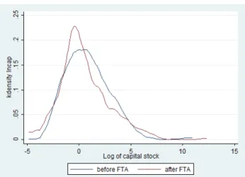
Figure 3 is for Malaysia. It seems the peak after the FTA is to the left of the one before the FTA.

Figure 3. Kernel density estimation of capital stock distribution for the investing Japanese firms (recipient country: Malaysia)

(13)

10

Figure 4 is for Chile. As shown, the peak of the size distribution after the FTA is clearly to the left of the one before the FTA with Chile. For Mexico and Chile as the locations for investment in the Americas, synergy and industrial agglomeration may still not be fully achieved. Thus, smaller-scale firms might have to move later than larger-scale firms under the FTA.

Figure 4. Kernel density estimation of capital stock distribution for the investing Japanese firms (recipient country: Chile)

Figure 5 is for Thailand. It seems that the average size of paid-up capital after the FTA is located slightly to the left of the average before the FTA.

Figure 5. Kernel density estimation of capital stock distribution for the investing Japanese firms (Recipient country: Thailand)

(14)

11

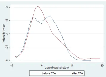
Figure 6 is for Indonesia. Two peaks appear in the distribution after the FTA, and the average size of paid-up capital cannot be seen clearly.

Figure 6. Kernel density estimation of capital stock distribution for the investing Japanese firms (recipient country: Indonesia)

Figure 7 is for the Philippines. The peak of the distribution after the FTA between the Philippines and Japan is located to the left of the one before the FTA.

Figure 7. Kernel density estimation of capital stock distribution for the investing Japanese firms (recipient country: Philippines)

(15)

12

Figure 8 is for Vietnam. The peak after the FTA is located to the left of the one before the FTA. The variance after the FTA seems to be bigger than the one before the FTA. Overall, the results are mixed in terms of statistical significance and also in terms of the direction of change.

Figure 8. Kernel density estimation of capital stock distribution for the investing Japanese firms (recipient country: Vietnam)

4. Statistical test of the average and variance of size distributions

Next, we statistically analyze the differences in means and variances of the size distributions. The statistical test of differences in firm-size average is presented first. Tables 1–8 show the results. Table 1 is for Singapore. As shown, the magnitude of the

t-value is below 2.0, meaning that there is no statistically significant difference before

(16)

13

Table 1. Two-sample t test of difference in averages with the assumption of equal variances for Singapore

Group | Obs. Mean Std. Err. Std. Dev. [95% Conf. Interval] 0 | 701 296.7191 138.3179 3662.16 25.15152 568.2868 1 | 260 914.5755 881.5757 14214.98 -821.3931 2650.544 combined | 961 463.8811 258.8098 8023.105 -44.01721 971.7794 diff | -617.8563 582.546 -1761.068 525.3557 diff = mean(0) - mean(1) t = -1.0606 Ho: diff = 0 degrees of freedom = 959 Ha: diff < 0 Ha: diff != 0 Ha: diff > 0

Pr(T < t) = 0.1446 Pr(|T| > |t|) = 0.2891 Pr(T > t) = 0.8554 Source: Calculated from Toyokeizai Shimposha’s database.

Table 2 is for Mexico. Just as in the case of Singapore, the t-value is not high enough to indicate a statistically significant change in the average of paid-up capitals after the FTA.

Table 2. Two-sample t test of difference in averages with the assumption of equal variances for Mexico

Group | Obs. Mean Std. Err. Std. Dev. [95% Conf. Interval] 0 | 160 56.47558 26.65178 337.1213 3.838423 109.1127 1 | 139 622.1824 547.1075 6450.302 -459.6152 1703.98 combined | 299 319.463 254.7732 4405.441 -181.9196 820.8457 diff | -565.7068 510.6131 -1570.585 439.1713 diff = mean(0) - mean(1) t = -1.1079 Ho: diff = 0 degrees of freedom = 297 Ha: diff < 0 Ha: diff != 0 Ha: diff > 0

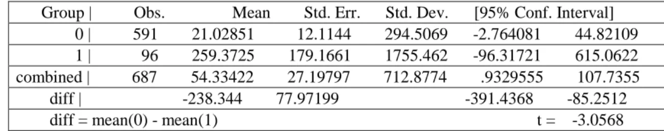
Table 3 is for Malaysia. Since the t value (-3.0568) has magnitude larger than 2, there is a structural change in the average value of paid-up capital.

Table 3. Two-sample t test of difference in averages with the assumption of equal variances for Malaysia

Group | Obs. Mean Std. Err. Std. Dev. [95% Conf. Interval] 0 | 591 21.02851 12.1144 294.5069 -2.764081 44.82109 1 | 96 259.3725 179.1661 1755.462 -96.31721 615.0622 combined | 687 54.33422 27.19797 712.8774 .9329555 107.7355 diff | -238.344 77.97199 -391.4368 -85.2512 diff = mean(0) - mean(1) t = -3.0568

(17)

14

Ho: diff = 0 degrees of freedom = 685 Ha: diff < 0 Ha: diff != 0 Ha: diff > 0

Table 4 is for Chile. Since the t-value (-3.1350) has magnitude larger than 2, the average has changed after the FTA.

Table 4. Two-sample t test of difference in averages with the assumption of equal variances for Chile

Group | Obs. Mean Std. Err. Std. Dev. [95% Conf. Interval] 0 | 37 57.83767 18.75039 114.0542 19.81012 95.86523 1 | 9 4464.685 2955.47 8866.41 -2350.641 11280.01 combined | 46 920.0469 609.8865 4136.451 -308.3275 2148.421 diff | -4406.847 1405.675 -7239.799 -1573.895 diff = mean(0) - mean(1) t = -3.1350 Ho: diff = 0 degrees of freedom = 44 Ha: diff < 0 Ha: diff != 0 Ha: diff > 0

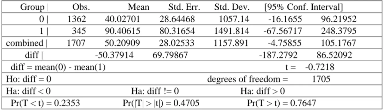
Table 5 is for Thailand. The t value is not large enough for statistical significance.

Table 5. Two-sample t test of difference in averages with the assumption of equal variances for Thailand

Group | Obs. Mean Std. Err. Std. Dev. [95% Conf. Interval] 0 | 1362 40.02701 28.64468 1057.14 -16.1655 96.21952 1 | 345 90.40615 80.31654 1491.814 -67.56717 248.3795 combined | 1707 50.20909 28.02533 1157.891 -4.75855 105.1767 diff | -50.37914 69.79867 -187.2792 86.52092 diff = mean(0) - mean(1) t = -0.7218 Ho: diff = 0 degrees of freedom = 1705 Ha: diff < 0 Ha: diff != 0 Ha: diff > 0

Table 6 is for Indonesia. The t value is not large enough in magnitude for statistical significance.

(18)

15

Indonesia

Group | Obs. Mean Std. Err. Std. Dev. [95% Conf. Interval] 0 | 584 41.62801 25.78878 623.2141 -9.022233 92.27824 1 | 231 6.829229 .7304664 11.10213 5.389968 8.26849 combined | 815 31.76479 18.48417 527.6897 -4.517453 68.04704 diff | 34.79878 41.02229 -45.7233 115.3209 diff = mean(0) - mean(1) t = 0.8483 Ho: diff = 0 degrees of freedom = 813 Ha: diff < 0 Ha: diff != 0 Ha: diff > 0

Table 7 is for the Philippines. As shown, the t-value for the test of average difference is low, and so the average size of the firm does not seem to have changed after the FTA.

Table 7. Two-sample t test of difference in averages with the assumption of equal variances for Philippines

Group | Obs. Mean Std. Err. Std. Dev. [95% Conf. Interval] 0 | 348 7.253982 .9954866 18.57056 5.296035 9.211929 1 | 42 5.661777 2.086904 13.52468 1.447189 9.876364 combined | 390 7.082513 .9158915 18.08741 5.281796 8.88323 diff | 1.592205 2.957271 -4.222076 7.406486 diff = mean(0) - mean(1) t = 0.5384 Ho: diff = 0 degrees of freedom = 388 Ha: diff < 0 Ha: diff != 0 Ha: diff > 0 Pr(T < t) = 0.7047 Pr(|T| > |t|) = 0.5906 Pr(T > t) = 0.2953 Source: Calculated from Toyokeizai Shimposha’s database.

Table 8 is for Vietnam. As shown, there is no statistically significant change in the average size of the firm (as characterized by paid-up capital) after the FTA.

Table 8. Two-sample t test of difference in averages with the assumption of equal variances for Vietnam

Group | Obs. Mean Std. Err. Std. Dev. [95% Conf. Interval] 0 | 407 674.9663 663.3645 13382.88 -629.0917 1979.024 1 | 180 11.83821 3.970356 53.26792 4.003489 19.67294 combined | 587 471.6221 459.9493 11143.69 -431.7277 1374.972 diff | 663.1281 997.9795 -1296.931 2623.187 diff = mean(0) - mean(1) t = 0.6645

Ho: diff = 0 degrees of freedom = 585 Ha: diff < 0 Ha: diff != 0 Ha: diff > 0

(19)

16

Next, we test whether the variance of the distribution has changed after FTA, using the F-test for equality of variances. Tables 9–16 show the results. Because in Table 9, the F-value of the ratio (0.0664) is not large enough, the variance is not significantly changed.

Table 9. Variance ratio test for Singapore

Group | Obs. Mean Std. Err. Std. Dev. [95% Conf. Interval] 0 | 701 296.7191 138.3179 3662.16 25.15152 568.2868 1 | 260 914.5755 881.5757 14214.98 -821.3931 2650.544 combined | 961 463.8811 258.8098 8023.105 -44.01721 971.7794 ratio = sd(0) / sd(1) f = 0.0664 Ho: ratio = 1 degrees of freedom = 700, 259 Ha: ratio < 1 Ha: ratio != 1 Ha: ratio > 1

Pr(F < f) = 0.0000 2*Pr(F < f) = 0.0000 Pr(F > f) = 1.0000 Source: Calculated from Toyokeizai Shimposha’s database.

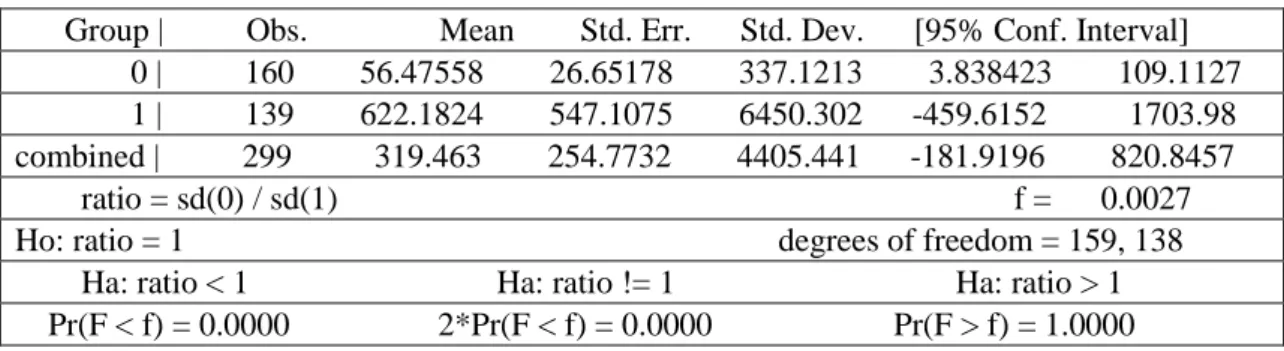
Table 10 is for Mexico. The result of the test is not statistically significant since the F-value (0.0027) is not high enough.

Table 10. Variance ratio test for Mexico

Group | Obs. Mean Std. Err. Std. Dev. [95% Conf. Interval] 0 | 160 56.47558 26.65178 337.1213 3.838423 109.1127 1 | 139 622.1824 547.1075 6450.302 -459.6152 1703.98 combined | 299 319.463 254.7732 4405.441 -181.9196 820.8457 ratio = sd(0) / sd(1) f = 0.0027 Ho: ratio = 1 degrees of freedom = 159, 138 Ha: ratio < 1 Ha: ratio != 1 Ha: ratio > 1 Pr(F < f) = 0.0000 2*Pr(F < f) = 0.0000 Pr(F > f) = 1.0000 Source: Calculated from Toyokeizai Shimposha’s database.

Table 11 is for Malaysia. The result is not statistically significant.

Table 11. Variance ratio test for Malaysia

Group | Obs. Mean Std. Err. Std. Dev. [95% Conf. Interval] 0 | 591 21.02851 12.1144 294.5069 -2.764081 44.82109 1 | 96 259.3725 179.1661 1755.462 -96.31721 615.0622 combined | 687 54.33422 27.19797 712.8774 .9329555 107.7355 ratio = sd(0) / sd(1) f = 0.0281

(20)

17

Ho: ratio = 1 degrees of freedom = 590, 95 Ha: ratio < 1 Ha: ratio != 1 Ha: ratio > 1 Pr(F < f) = 0.0000 2*Pr(F < f) = 0.0000 Pr(F > f) = 1.0000 Source: Calculated from Toyokeizai Shimposha’s database.

Table 12 is for Chile. The F value to be tested is 0.0002, which is not high enough to make the test statistically significant.

Table 12. Variance ratio test for Chile

Group | Obs. Mean Std. Err. Std. Dev. [95% Conf. Interval] 0 | 37 57.83767 18.75039 114.0542 19.81012 95.86523 1 | 9 4464.685 2955.47 8866.41 -2350.641 11280.01 combined | 46 920.0469 609.8865 4136.451 -308.3275 2148.421 ratio = sd(0) / sd(1) f = 0.0002 Ho: ratio = 1 degrees of freedom = 36, 8 Ha: ratio < 1 Ha: ratio != 1 Ha: ratio > 1

Pr(F < f) = 0.0000 2*Pr(F < f) = 0.0000 Pr(F > f) = 1.0000 Source: Calculated from Toyokeizai Shimposha’s database.

Table 13 is for Thailand. As the F value (0.5022) is not high enough, the result is not statistically significant.

Table 13. Variance ratio test for Thailand

Group | Obs. Mean Std. Err. Std. Dev. [95% Conf. Interval] 0 | 1362 40.02701 28.64468 1057.14 -16.1655 96.21952 1 | 345 90.40615 80.31654 1491.814 -67.56717 248.3795 combined | 1707 50.20909 28.02533 1157.891 -4.75855 105.1767 ratio = sd(0) / sd(1) f = 0.5022 Ho: ratio = 1 degrees of freedom = 1361, 344 Ha: ratio < 1 Ha: ratio != 1 Ha: ratio > 1 Pr(F < f) = 0.0000 2*Pr(F < f) = 0.0000 Pr(F > f) = 1.0000 Source: Calculated from Toyokeizai Shimposha’s database.

Table 14 is for Indonesia. The F-value for the ratio (3.2e+03, or 3.2 x 103) is large enough to make this test statistically significant; thus, it seems that there was a change in variance after the FTA.

Table 14. Variance ratio test for Indonesia

Group | Obs. Mean Std. Err. Std. Dev. [95% Conf. Interval] 0 | 584 41.62801 25.78878 623.2141 -9.022233 92.27824 1 | 231 6.829229 .7304664 11.10213 5.389968 8.26849

(21)

18

combined | 815 31.76479 18.48417 527.6897 -4.517453 68.04704 ratio = sd(0) / sd(1) f = 3.2e+03 Ho: ratio = 1 degrees of freedom = 583, 230 Ha: ratio < 1 Ha: ratio != 1 Ha: ratio > 1 Pr(F < f) = 1.0000 2*Pr(F > f) = 0.0000 Pr(F > f) = 0.0000 Source: Calculated from Toyokeizai Shimposha’s database.

Table 15 is for the Philippines. The F-value of the ratio (1.8854) is high enough for the degrees of freedom in this test, and therefore the variance change is taken as statistically significant.

Table 15. Variance ratio test for Philippines

Group | Obs. Mean Std. Err. Std. Dev. [95% Conf. Interval] 0 | 348 7.253982 .9954866 18.57056 5.296035 9.211929 1 | 42 5.661777 2.086904 13.52468 1.447189 9.876364 combined | 390 7.082513 .9158915 18.08741 5.281796 8.88323 ratio = sd(0) / sd(1) f = 1.8854 Ho: ratio = 1 degrees of freedom = 347, 41 Ha: ratio < 1 Ha: ratio != 1 Ha: ratio > 1 Pr(F < f) = 0.9925 2*Pr(F > f) = 0.0150 Pr(F > f) = 0.0075 Source: Calculated from Toyokeizai Shimposha’s database.

Table 16 is for Vietnam. The change in variance is statistically significant for Vietnam since the F-value is large enough.

Table 16. Variance ratio test for Vietnam

Group | Obs. Mean Std. Err. Std. Dev. [95% Conf. Interval] 0 | 407 674.9663 663.3645 13382.88 -629.0917 1979.024 1 | 180 11.83821 3.970356 53.26792 4.003489 19.67294 combined | 587 471.6221 459.9493 11143.69 -431.7277 1374.972 ratio = sd(0) / sd(1) f = 6.3e+04 Ho: ratio = 1 degrees of freedom = 406, 179 Ha: ratio < 1 Ha: ratio != 1 Ha: ratio > 1 Pr(F < f) = 1.0000 2*Pr(F > f) = 0.0000 Pr(F > f) = 0.0000 Source: Calculated from Toyokeizai Shimposha’s database.

The results are summarized in Table 17. The results are mixed, to say the least. For Malaysia and Chile, the test for average difference is significant. For Indonesia, the Philippines and Vietnam, the test for the difference in variance is significant. For all other countries, the results are not statistically significant.

(22)

19

terms of paid-up capital stock) FTA partner country

Test for the difference of mean

Test for the difference of variance

Singapore Not significant Not significant Mexico Not significant Not significant Malaysia Significant Not significant Chile Significant Not significant Thailand Not significant Not significant Indonesia Not significant Significant Philippines Not significant Significant Vietnam Not significant Significant Source: Calculated from Toyokeizai Shimposha’s database.

5. Conclusions and policy implications

This paper has examined the determinants of FDI under FTAs from a new institutional perspective. The statistical analysis of FDI at the aggregate level reveals that there is some evidence of “structural changes” after FTAs in terms of the investing firms’ paid-up capital stock. The statistical test for changes in the average and variance of the size distribution confirms this in the case of FTAs with Asian partner countries. Overall, it seems that the impact of FTA on the size of the investing firms is somewhat non-linear.

As for FTAs with South American countries (Mexico and Chile), it seems the existence of FTAs seems to promote larger-scale FDIs in order to establish industrial agglomeration. These results remain correlational instead of causal, and more statistical analyses is needed for further understanding. Among policy implications, participating firms should consider institutional aspects of FTAs, such as size as a determinant of FDI. Theoretically speaking, FDI is a non-market solution to market imperfection. To adapt to the local business environment, firms are seen to change in size. The empirical observations and the results of the statistical tests are only partially in line with the theoretical hypothesis. Future work along this line is therefore much needed, particularly with regard to firm heterogeneity as characterized by firm size.

(23)

20

References:

Casson, Mark (1986), “General Theories of the Multinational Enterprise: Their Relevance to Business History”, in Peter Hertner and Geoffrey Jones (eds.),

Multinationals: Theory and History, Aldershot: Gower, pp. 42-63.

Casson, Mark (1987), The Firm and the Market: Studies on Multinational Enterprise

and the Scope of the Firm, Oxford: Basil Blackwell.

Dunning, John H. (1992), Multinational Enterprises and the Global Economy, Wokingham, England: Addison-Wesley Publishing.

Melitz, Marc (2003), “The Impact of Trade on Intra-Industry Reallocations and Aggregate Industry Productivity”, Econometrica, vol. 71 no. 6, pp. 1695-1725. Stiglitz, Joseph E. and Andrew Charlton (2005), Fair Trade for All: How Trade can

Promote Development, Oxford New York: Oxford University Press.

Tejima, Shigeki (1998), “Chokusetsu-Toshi to Keizai Kaihatsu” (Foreign Direct Investment and Economic Development), Kaigai Toshi Kenkyujo Ho, pp. 4 – 48.