How serious is the omission of bilateral
tariff rates in gravity?
著者
Hayakawa Kazunobu
権利
Copyrights 日本貿易振興機構(ジェトロ)アジア
経済研究所 / Institute of Developing
Economies, Japan External Trade Organization
(IDE-JETRO) http://www.ide.go.jp
journal or
publication title
IDE Discussion Paper
volume
311
year
2011-10-01
INSTITUTE OF DEVELOPING ECONOMIES
IDE Discussion Papers are preliminary materials circulated to stimulate discussions and critical comments
Keywords: Gravity; Tariff rates; Free Trade Agreement
JEL classification: F10; F15
* Bangkok Research Center, Japan External Trade Organization, Thailand, ([email protected])
Abstract: In this paper, using the worldwide dataset of bilateral tariff rates, we explore how serious the omission of bilateral tariff rates in gravity is. Our findings are as follow. Firstly, the omission of bilateral tariff rates seems not to be so serious in terms of omitted-variable biases because the coefficients for the usual gravity variables do not change before or after their inclusion. Secondly, while the widely-used dummy variable of regional trade agreement could not play an alternative role in place of tariff rates, the inclusion of time-invariant pair fixed effects in addition to the time-variant importer fixed effects and exporter fixed effects accounts for the omission of tariff rates. The inclusion of those fixed effects makes the coefficient for bilateral tariff rates insignificant.
IDE DISCUSSION PAPER No. 311
How Serious Is the Omission of
Bilateral Tariff Rates in Gravity?
Kazunobu HAYAKAWA*
The Institute of Developing Economies (IDE) is a semigovernmental, nonpartisan, nonprofit research institute, founded in 1958. The Institute merged with the Japan External Trade Organization (JETRO) on July 1, 1998.
The Institute conducts basic and comprehensive studies on economic and related affairs in all developing countries and regions, including Asia, the Middle East, Africa, Latin America, Oceania, and Eastern Europe.
The views expressed in this publication are those of the author(s). Publication does not imply endorsement by the Institute of Developing Economies of any of the views expressed within.
INSTITUTE OF DEVELOPING ECONOMIES (IDE), JETRO
3-2-2, WAKABA,MIHAMA-KU,CHIBA-SHI
CHIBA 261-8545, JAPAN
©2011 by Institute of Developing Economies, JETRO
No part of this publication may be reproduced without the prior permission of the IDE-JETRO.
1
1. Introduction
In international economics, the ‘gravity equation’ has been considered to be the most powerful empirical tool for investigating the determinants of bilateral trade values. The traditional gravity equation has a log of bilateral trade as a dependent variable as well as logs of importer’s and exporter’s GDPs and a log of distance between trading partners as independent variables. Its estimation always presents us with an excellent empirical fit. Relying on such properties, a large number of scholars have employed the gravity equation for the investigation of bilateral trade. It can be used for clarifying the causes of growth of world trade after the Second World War (Baier and Bergstrand 2001). The impact of international agreements such as free trade agreements (FTAs) (Baier and Bergstrand 2007) and of international organizations such as the World Trade Organization (Rose 2004) on trade can also be evaluated by the gravity equation. The development of these gravity papers proves the equation’s usefulness in empirical analysis. In addition, there are now a variety of the theoretical models supporting the gravity formulation (see, for example, Combes et al. 2008: 127). In short, a gravity equation is a powerful tool from both the theoretical and empirical points of view.
However, no studies heretofore have included the most important economic variable in international economics, bilateral tariff rates, in the gravity equation. The study of international economics belongs to regional economics, but an important difference between it and other fields in regional economics such as urban economics is that the boundaries of the regions are national borders, not city borders or state borders. Thus, in international economics, theoretical models show that transactions across regional boundaries require firms to incur ‘trade costs.’ In particular, in contrast to other fields in regional economics, trade costs in international economics include not only physical transport costs but also policy-related costs, namely, tariff and non-tariff barriers. So, tariff rates are the most important economic variable in international economics in terms of the differentiation with other fields in regional economics. In spite of such importance, the gravity studies in international economics have never included time-variant trading pair-specific tariff rates. This means that our previous estimators in gravity may suffer from serious omitted-variable biases: if any elements affecting bilateral tariff rates are related to other gravity variables, the coefficients for those variables suffer from biases due to the omission of the tariff rates.
The obvious reason for such omission of bilateral tariff rates in the gravity analysis lies in the data availability. Countries have several kinds of tariff duty and levy different kinds of duty on each trading partner country. The major kinds of tariff duty include most-favored nation (MFN) rates, generalized system of preferences (GSP)
2
rates, and FTA preferential rates. Based on whether trading partners are members of the World Trade Organization (WTO), are developing countries, and/or share membership in the same FTA, we need to classify each trading partner’s applied tariff schemes. Thus, what we firstly need to do is to collect all kinds of tariff duty information for each country. Although each country reports this information, worldwide collection of it has presented a huge task. Even if we successfully collected such data, we then would need to carry out the above-mentioned classification of tariff schemes according to trading partners. In short, although tariff rates are the most important variable in international economics, measures of them are also one of the most difficult measures to construct. Recently, there have been some efforts toward the construction of a database of tariff rates. As listed in Bouet et al. (2005), several databases of tariff rates exist: Hemispheric Database by Inter-American Development Bank; Integrated Database (IDB) by the WTO; Integrated Tariff Analysis System (ITAS) by the Australian Government Productivity Commission; MAcMap by the Centre d’Informations Internationales (CEPII); and Trade Analysis and Information System (TRAINS) by the United Nations Conference on Trade And Development (UNCTAD). In particular, the World Integrated Trade Solution (WITS)1 is now the most powerful software developed by the World Bank, UNCTAD, International Trade Center (ITC), United Nations Statistical Division (UNSD), and WTO. This database includes tariff, para-tariff, and non-tariff measures at the national tariff line level by origin for more than 200 countries. In short, the above-mentioned difficulties in constructing bilateral tariff data could be overcome by employing this database. It is expected that this database will become the major data source for tariff data in international economics. In this paper, using the worldwide dataset of bilateral tariff rates drawn from the WITS, we explore how serious the omission of bilateral tariff rates in gravity is. Specifically, we firstly examine how coefficients for other variables such as geographical distance change before and after the introduction of bilateral tariff rates. That is, we explore how large the biases from the omission of bilateral tariff rates are. Secondly, we investigate whether or not the inclusion of a dummy variable for regional trade agreement (RTA) plays an alternative role by representing the inclusion of bilateral tariff rates. Compared with the bilateral tariff rates, it is easy to construct the RTA dummy, which takes unity if two countries are members of the same RTA and zero otherwise. Indeed, one of the crucial sources for heterogeneous tariff rates across trading partners is the existence of RTA. If the simple one-zero RTA dummy, which has been included in some of the previous studies in gravity, is able to explain most of the
1
3
variation in bilateral tariff rates, the inclusion of the RTA dummy will account for the omission of bilateral tariff rates. In place of RTA dummy variables, we also attempt to include some kinds of fixed effects to examine whether or not those fixed effects could play an alternative role by representing bilateral tariff rates.
The rest of this paper is organized as follows. The next section presents an overview of bilateral tariff rates around the world. In Section 3, we estimate several gravity equations, and Section 4 examines the seriousness of the omission of bilateral tariff rates in gravity. In Section 5, the conclusion of this paper is presented.
2. Bilateral Tariff Rates
This section presents an overview of manufacturing tariff rates around the world. Our data source for tariff rates is the WITS, particularly TRAINS raw data. In addition, some other sources are used for identifying exact tariff schemes for each trading partner.2 In particular, we needed to make a list of member countries in the WTO and in each RTA. Also, the GSP beneficiaries are different across importers. The information regarding the WTO and RTA is obtained from the WTO website. We used the ‘Regional Trade Agreements Information System’ for obtaining the member list of each RTA.3 As for the GSP beneficiaries, we used several documents available on the UNCTAD website in addition to official documents on the website of national customs agencies in each country.4 Notice that we take into account only GSP beneficiaries which can be identified in these documents. While the lists of beneficiary countries are commonly available for one specific year in each country, the beneficiary countries may change over time, i.e., they may graduate from being GSP beneficiaries. Therefore, we may undercount/overcount GSP beneficiaries.
It is further worth noting three points. Firstly, a different version of the Harmonized System (HS) is used depending on the year in each country. In order to construct a tariff database comparable across years, we convert all HS versions (HS1996, HS2002, and HS2007) to HS1992 using the HS conversion tables available at the UNSD.5 As a result, our background database of bilateral tariff rates is constructed
2
We assume that all firms use the tariff schemes with the lowest rates, though some firms may be forced to use the higher general tariff rates such as MFN rates because it is necessary to incur some kinds of fixed costs for the use of preferential tariff schemes (Demidova and Krishna 2008).
3 http://rtais.wto.org/UI/PublicMaintainRTAHome.aspx 4 http://www.unctad.org/Templates/Page.asp?intItemID=1418&lang=1 5 http://unstats.un.org/unsd/trade/conversions/HS%20Correlation%20and%20Conversion%20tables.ht m
4
at the 6-digit level of HS1992. Secondly, we put the most recent past rates available into missing data. For example, if tariff data are missing in 2000 and 2001 during the period of 1996-2006, we use the rates in 1999 for rates in 2000 and 2001. Thirdly, we treat non-ad valorem tariff rates simply as missing. Also, for simplicity, we use the lower rates for mix tariff rates, though these treatments underestimate tariff rates to some extent.
We aggregate 6-digit level tariff rates into a single tariff rate for the manufacturing industry by the using the simple average of 6-digit level manufactured products. The manufacturing industry includes Sectors 2 to 4 of the CPC provisional classification6 using the conversion table for HS1992, available on the website of UNSD.7 Our focus on the manufacturing industry obviously decreases the magnitude of the above-mentioned underestimation because non-ad valorem tariff rates and mix tariff rates are mostly set in non-manufacturing industries. As a result, our database of bilateral tariff rates in the manufacturing industry is a completely-balanced panel dataset for 94 countries (see Appendix) and 11 years (1996-2006).
Let us start by examining two figures. The average of bilateral tariff rates in all sample pairs is depicted in Figure 1, which shows a steady decrease from 1996 to 2006. The rates decreased by half, from 14% in 1996 to 7% in 2006. Figure 2 shows the ranking of the average bilateral tariff rates in each importing country in 2006. More than a half of the sample countries have average tariff rates of less than 10%. The well-known champions of openness are ranked first, namely Hong Kong, Singapore, and Switzerland, followed by the member counties of the European Union (EU). Countries that rank third in openness include high income countries, such as Japan, the USA, and oil countries (e.g., Brunei and Saudi Arabia). The less developed countries are also less open countries in terms of bilateral tariff rates.
=== Figures 1&2 ===
Table 1 shows the inter- and intra-continental/regional tariff rates in 1996 and 2006. Taking a look at intra-regional tariff rates, i.e., ‘Within Region,’ we see three noteworthy points. Firstly, Europe and the Pacific regions have had rather low tariff rates (however, notice that the Pacific region consists of only two countries in our sample). Particularly in 2006, those regions had tariff rates of less than 1%. Secondly,
6
Sector 2 is food products, beverages and tobacco as well as textiles, apparel and leather products; Section 3 is other transportable goods, except metal products, machinery and equipment; Sector 4 is metal products, machinery and equipment.
7
5
while the intra-regional tariff rates in Asia were the highest (21%) among the five regions, those rates dramatically dropped to 8% in 2006, which is almost the same level as those in America. Some reasons for this dramatic drop may be the acceleration of tariff reduction in the ASEAN Free Trade Area, China’s admittance to the WTO, several FTAs concluded among oil countries, and so on.
=== Table 1 ===
The inter-regional tariff rates are also reported in Table 1. The column ‘To Outside Region’ reports the tariff rates applied when each region exports to the outside. Countries in Europe and the Pacific have needed to pay much higher tariff rates when exporting to the outside than when exporting to intra-regional countries. On the other hand, African countries have had better access to outside countries than to intra-regional countries. In 2006, there is little gap in America and Asia between inter-regional access and intra-regional access. The column ‘From Outside Region’ indicates the tariff rates applied to countries outside of each region. In this column, we can see a ‘regional block’: inter-regional tariff rates are higher than intra-regional tariff rates. However, the magnitude of the gap between those kinds of tariff rates is trivial, at only 1% to 2%.
3. Gravity
In international economics, it is well known that a gravity equation is one of the most successful tools for quantitatively analyzing bilateral merchandise trade patterns. The traditional gravity equation has logs of the importer’s and exporter’s GDPs and a log of distance between trading partners:
ln Tij = β0 + β1 ln GDPi + β2 ln GDPj + β3 ln Distanceij + εij,
where Tij represents bilateral goods exports of country i to country j. Its estimation always presents us with an excellent empirical fit. Relying on such properties, a large number of scholars have employed the gravity equation for the investigation of bilateral trade. This gravity equation is often extended as follows:
ln Tij = β0 + β1 ln GDPi + β2 ln GDPj + β3 ln Distanceij + β4 Contingencyij
+ β5 Languageij + β6 Colonyij + εij. (1) Contingency takes unity if two countries share the national border and zero otherwise. Language is a dummy variable taking unity if a language is spoken by at least 9% of the population in both countries and zero otherwise. Colony takes unity if two countries had colonial relationship in the past and zero otherwise.
6
It is well known that this gravity equation can be supported by various kinds of theoretical models. Anderson (1979) and Bergstrand (1985, 1989), in which gravity models are based on the Armington assumption (1969), are amongst the classics. Subsequently, it has been shown that the gravity equation can be derived from many different models, including the Ricardian (Eaton and Kortum 2002), Heckscher–Ohlin (Deardorff 1998), and monopolistic competition models (Helpman and Krugman 1985). In particular, under the usual assumptions in horizontal differentiation models (e.g., CES utility function), Anderson and van Wincoop (2003) derive the following gravity equation (equation 9 on page 175):
1 j i ij W j i ij P t y y y x , (2) where
1 1 1 j ij j j i t P ,
1 1 1 i ij i i j t P , and j yj yW .xij, yi, tij, and yW are the nominal value exports from countries i to j, total income of country i, iceberg trade costs from countries i to j, and world nominal income, respectively. σ denotes the elasticity of substitution among varieties. Π and P are price indices and are also called ‘multilateral resistance’ terms.
Taking logs in equation (2), we obtain:
ij
i
j j i W ij y y y t P x ln ln ln 1 ln 1ln 1ln ln .The usual assumption is that trade costs t are log-linear to geographical distance, linguistic commonality, colonial relationship, and border contingency;
tan 1 exp
2
exp
3
exp 4
exp0 ij ij ij ij
ij Dis ce Contingency Language Colony
t .
Then, this equation can be rewritten as:
ln Tij = β0 + β1 ln GDPi + β2 ln GDPj + β3 ln Distanceij + β4 Contingencyij
+ β5 Languageij + β6 Colonyij + β7 ln Πi + β8 ln Pj + εij. (3) GDP is used as a proxy for y. Compared with the traditional equation (1), this theory-based equation includes multilateral resistance terms, namely ln Πi and ln Pj. In order to control these terms, we follow the method proposed by Feenstra (2002), which replaces multilateral resistance variables with importer and exporter dummies. Thus, the equation to be usually estimated can be shown as:
ln Tij = β0 + β3 ln Distanceij + β4 Contingencyij + β5 Languageij
7
The inclusion of importer and exporter dummy variables forces us to drop importer and exporter GDPs.
However, we do not have any convincing empirical evidence that trade costs do not depend on bilateral tariff rates. Since tariff rates are not identical all over the world, and furthermore, not importer-specific, the constant term and importer fixed effects do not take care of the omission of tariff rates at all. In short, in the usual gravity estimation, bilateral tariff rates are included in the error term. Therefore, if unobservable shocks to bilateral tariff rates are also related to other gravity variables, their coefficients are biased. For example, developed countries might be likely to give GSP status to countries with a colonial relationship. In order to check the magnitude of such biases, we naturally assume that trade costs depend further on bilateral tariff rates;
ij
ij
ij
ij
ij
ij Dis ce Contingency Language Colony Tariff
t exp tan 1exp 2 exp 3 exp 4 1
0 .
Then, the gravity equation is given by:
ln Tij = β0 + β3 ln Distanceij + β4 Contingencyij + β5 Languageij
+ β6 Colonyij + β9 ln (1+Tariffij) + ui + uj + εij. (5) Comparing the estimated coefficients between (4) and (5), we investigate how serious the omission of bilateral tariff rates is in the gravity estimation.
We estimate the above-listed gravity equations for manufacturing trade among 94 countries during 1996-2006. Our data sources are as follow. The bilateral trade values are obtained from the UN Comtrade. As in the case of tariff rates, we examine bilateral trade in the manufacturing industry based on CPC provisional classification. Thus, bilateral trade values at 6-digit HS1992 level are aggregated to those in the manufacturing industry. In the recent literature on gravity, zero-valued trade is a hot issue. In our case, around 20% of the country pairs have zero-valued trade in the manufacturing industry. Although this is not a trivial amount, we drop those pairs for simplicity. However, the simple treatment of adding the value of one before taking a log does not change our estimation results presented in the next section.8 The data source for bilateral tariff rates is the same as in Section 2. The sources for Distance, Contingency, Language, and Colony are on the CEPII website.
8
The approach adopted in the recent literature for addressing this issue is the use of the method proposed by Silva and Tenreyro (2006) or Helpman, Melitz, and Rubinstein (2008). While the former approach is the pseudo poisson maximum likelihood technique, the latter one is the extended technique of the Heckman two-step estimation. In this paper, we do not take this issue into account because it is difficult to obtain the convergence of log-likelihood in such maximum likelihood techniques for our model which includes three kinds of fixed effects (we will introduce uit, ujt, and uij) and a large number of countries and years.
8
4. Estimation Results
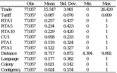
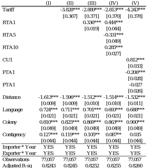
This section reports the estimation results of several gravity equations. The basic statistics and our baseline results are reported in Tables 2 and 3, respectively. Column (I) in Table 3 reports the results of equation (4), namely the gravity equations without tariff rates. All coefficients are significantly estimated with expected signs. The geographical distance between trading partners is negatively correlated with trade values. The linguistic commonality, colonial relationship, and sharing the national border encourage active trade between two countries. This model explains well the bilateral trade flows all over the world; adjusted R-squared registers more than 80%. These results are the same as the ones that we always obtained in previous studies.
=== Tables 2 & 3 ===
In column (II), we include bilateral tariff rates in the gravity equation, i.e., equation (5). The coefficient for bilateral tariff rates is estimated to be significantly negative, as is consistent with our expectation. From the theoretical point of view underlying the gravity equation, as demonstrated in the previous section, its coefficient can be directly related to the elasticity of substitution among goods/varieties (σ). Specifically, it is equal to 1-σ. Thus, σ implied by our estimator becomes approximately 5, which is a reasonable value in the literature.9 The results in the other variables are almost the same as those in column (I). In particular, the magnitude of coefficients for those variables does not change significantly. For example, the coefficient for Distance changes only from -1.613 to -1.596. Also, the adjusted R-squared does not experience a remarkable rise, compared with that in column (I). In short, while the bilateral tariff rates are important in terms of model specification because of their significant impacts on trade values, their omission seems to be not so serious in terms of biases in other gravity variables and in terms of of the empirical fit of the gravity model.
Next, we examine whether or not the inclusion of RTA dummy variables, which are easier to construct than bilateral tariff rates, makes the coefficient for bilateral tariff rates insignificant. The widely-used measure for RTAs is a one-zero RTA dummy, which takes unity if two countries are members of the same RTA and zero otherwise. If its inclusion makes the coefficient for the tariff rates insignificant, the omission of bilateral
9
Head and Ries (2001) and Hanson (2005) obtain estimates of σ ranging between 7 and 11 and between 5 and 8, respectively. As a result, Anderson and van Wincoop (2004) conclude that σ is likely to be in the range of 5 to 10.
9
tariff rates does not matter because the RTA dummy plays an alternative role in place of bilateral tariff rates. We construct the RTA dummy by using the list of RTAs provided on the WTO website under ‘The Regional Trade Agreements Information System,’ as used in Section 2. This list is based on notifications from the WTO member countries and provides data on both active and inactive (or vanished) RTAs. This implies that RTAs not reported to GATT/WTO are not incorporated into our dataset. Furthermore, while our RTA dummy includes RTAs reported under GATT Article XXIV as well as the Enabling Clause, RTAs reported under GATS Article V are excluded.
The results of the simple introduction of a one-zero RTA dummy variable, which is one-year lagged, are reported in column (III). The coefficient for Tariff is still significantly negative, and its absolute magnitude drops remarkably due to the inclusion of the RTA dummy variable. The latter result implies that the variation of bilateral tariff rates is partly explained by the RTA dummy variable. The coefficient for RTA is also estimated to be significantly positive, as is consistent with our expectation. In column (IV), we introduce further lagged RTA dummy variables (five-year lagged and ten-year lagged) in order to take into account a ‘phase-in’ period in RTAs. However, the results are qualitatively unchanged, though the coefficient for the five-year lagged RTA dummy is estimated to be negatively significant. Compared with (I), these equations with RTA dummy variables have different absolute values in the coefficients for other standard gravity variables, particularly Distance, but these changes come from the inclusion of RTA dummy variables, not the inclusion of bilateral tariff rates, as confirmed in (II). Thus, RTA dummy variables may capture the more significant portion of trade creation effects than bilateral tariff rates. In other words, the omission of RTA dummy variables may be more serious than the omission of bilateral tariff rates in terms of biases in other gravity variables.
In addition, we take into account the heterogeneity of RTAs to some extent as in Vicard (2009). Specifically, we decompose a simple RTA dummy variable into CU dummy (one for the same Customs Union members), FTA dummy (one for the same Free Trade Agreement members), and PTA dummy variables (one for the same Preferential Trade Agreement members).10 This decomposition is also possible with the information from the above-mentioned WTO website. The estimation results in this case are reported in column (V) and show again the negatively significant impacts of bilateral tariff rates on trade values. The Customs Union shows the largest trade creation effects, though the coefficient for FTA is estimated to be significantly negative. The
10
CU is defined in Paragraph 8(a) of Article XXIV of GATT 1994, FTA is defined in Paragraph 8(b) of Article XXIV of GATT 1994, and PTA is reported under paragraph 4(a) of the Enabling Clause.
10
coefficient for Contingency turns out to be insignificant. As a result, we can say that the omission of bilateral tariff rates does not yield serious biases in other standard gravity variables, but should be avoided because of their significant impacts on trade values.
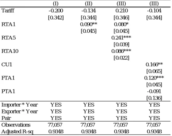
Lastly, we introduce time-invariant country pair fixed effects instead of RTA dummy variables. Then, time-invariant pair specific explanatory variables, i.e., all variables other than tariff rates, are dropped. The result is reported in column (I) in Table 4. Interestingly, the coefficient for Tariff turns out to be insignificant, though its sign is still negative. This insignificant result implies that a significant part of the impacts of bilateral tariff rates could be explained by time-invariant pair specific elements. The inclusion of some RTA dummy variables makes the result in bilateral tariff rates all the more insignificant, as found in columns (II)-(IV).11 In sum, if including time-varying exporter fixed effects, time-varying importer fixed effects, and time-invariant pair fixed effects, the omission of bilateral tariff rates in gravity equations does not matter at all because those fixed effects can play an alternative role in place of the tariff rates.
=== Table 4 ===
This insignificant result in bilateral tariff rates might be reasonable because GSP status, WTO membership, and those tariff rates do not change so frequently, particularly during a period of about 10 years like our sample. As a result, those impacts are mostly controlled by time-invariant pair fixed effects. Even if the impacts of GSP and WTO membership are completely controlled, however, the variation of tariff rates through RTAs is still expected to have significant impacts on trade values. Thus, the insignificant results imply that RTAs do not explain a significant part of bilateral tariff rates. In order to confirm this hypothesis, we investigate to what degree the RTA dummy variables can explain the variation of bilateral tariff rates by regressing RTA
11
It is well known that the introduction of a time-invariant pair dummy also accounts for the endogeneity issue in RTA variables: elements having influence on international trade between them also affect the decision on the RTA conclusion (see Baier and Bergstrand 2004, 2007). Baier and Bergstrand (2007) closely examine this issue. One possible way of addressing the endogeneity is the use of instruments. Baier and Bergstrand (2007) tried a wide array of economic and political instrument variables. However, they conclude that the instrument variable method is not a reliable method because of the lack of suitable instruments. Most of the variables that are correlated cross-sectionally with the probability of having an RTA are also correlated cross-sectionally with trade flows. As a result, they demonstrate that the most plausible estimates of the RTA impacts on international trade are obtained from the gravity estimation using panel data with bilateral fixed effects. This estimation enables us to isolate the RTA impacts on bilateral international trade from any time-invariant country-pair-specific elements, some of which are related with the decision on the conclusion of the RTA and bilateral international trade.
11
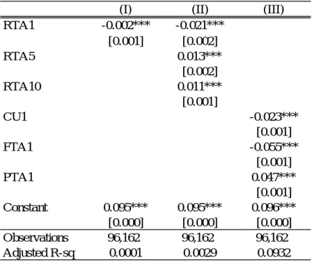
dummy variables on bilateral tariff rates. The OLS results are reported in Table 5. Column (I) is the result for the simple equation including a simple one-year lagged RTA dummy. The coefficient for the RTA dummy is negatively significant. However, adjusted R-squared is just 0.01%, indicating that the simple RTA dummy does little to explain the variation of bilateral tariff rates. In columns (II) and (III), we introduce the further-lagged RTA dummy variables and the decomposed RTA dummy variables, respectively. Although some variables have unexpected signs, these RTA dummy variables could explain, at most, 10% of the variation of bilateral tariff rates. Thus, such trivial contribution by RTAs may yield the insignificant impacts of bilateral tariff rates when including time-invariant pair fixed effects.
=== Table 5 ===
5. Concluding Remarks
In this paper, using the worldwide dataset of bilateral tariff rates, we explore the seriousness of the omission of bilateral tariff rates in gravity. Two kinds of analyses were conducted. The first one was to explore how large the biases from the omission of bilateral tariff rates are. Secondly, we investigate whether or not RTA dummy variables or some fixed effects play an alternative role in place of bilateral tariff rates. As a result, we found that the omission of bilateral tariff rates seems not to be particularly serious in terms of omitted-variable biases because the coefficients for standard gravity variables do not change qualitatively and quantitatively between gravity equations with or without tariff rates. Furthermore, while RTA dummy variables cannot play an alternative role in place of tariff rates, the inclusion of time-invariant pair fixed effects in addition to the time-variant importer fixed effects and exporter fixed effects accounts for the omission of tariff rates because the gravity equation with those three kinds of fixed effects does not yield significant results in the tariff rates. In short, without data on bilateral tariff rates, it is recommended that the gravity equation be estimated with those three kinds of fixed effects.
12
Appendix: Sample Countries
Region Country Region Country
Africa Burkina Faso Asia Bangladesh
Africa Gabon Asia Brunei Darussalam
Africa Ghana Asia China
Africa Kenya Asia Hong Kong
Africa Madagascar Asia India
Africa Malawi Asia Indonesia
Africa Mali Asia Israel
Africa Mauritius Asia Japan
Africa Morocco Asia Korea
Africa Nigeria Asia Malaysia
Africa Rwanda Asia Nepal
Africa South Africa Asia Oman
Africa Tanzania, United Rep. of Asia Pakistan
Africa Tunisia Asia Philippines
Africa Uganda Asia Saudi Arabia
Africa Zambia Asia Singapore
Africa Zimbabwe Asia Sri Lanka
America Argentina Asia Thailand
America Barbados Asia Viet Nam
America Belize Europe Belgium and Luxembourg
America Bolivia Europe Czech Republic
America Brazil Europe Denmark
America Canada Europe Estonia
America Chile Europe Finland
America Colombia Europe France
America Costa Rica Europe Germany
America Dominica Europe Greece
America Ecuador Europe Hungary
America El Salvador Europe Iceland
America Grenada Europe Ireland
America Guatemala Europe Italy
America Guyana Europe Latvia
America Honduras Europe Lithuania
America Jamaica Europe Luxembourg
America Mexico Europe Moldova, Rep.of
America Nicaragua Europe Netherlands
America Paraguay Europe Norway
America Peru Europe Poland
America Saint Kitts and Nevis Europe Portugal
America Saint Lucia Europe Romania
America Saint Vincent and the Grenadines Europe Spain
America Suriname Europe Sweden
America Trinidad and Tobago Europe Switzerland America United States of America Europe Turkey
America Uruguay Europe Ukraine
America Venezuela Europe United Kingdom Pacific Australia Pacific New Zealand
13
References
Anderson, J.E., 1979, A Theoretical Foundation for the Gravity Equation, American Economic Review, 69(1): 106-116.
Anderson, J. E. and van Wincoop, E., 2003, Gravity with Gravitas: A Solution to the Border Puzzle, American Economic Review, 93(1): 170-192.
Anderson, J. E. and van Wincoop, E., 2004, Trade Costs, Journal of Economic Literature, 42: 691–751.
Armington, P. S., 1969, A Theory of Demand for Products Distinguished by Place of Production, IMF Staff Papers, 16: 159-178.
Baier, S.L. and Bergstrand, J.H., 2004, Economic Determinants of Free Trade Agreements, Journal of International Economics, 64(1): 29-63.
Baier, S.L. and Bergstrand, J.H., 2007, Do Free Trade Agreements Actually Increase Members’ International Trade?, Journal of International Economics, 71(1): Bergstrand, J.H., 1985, The Gravity Equation in International Trade: Some
Microeconomic Foundations and Empirical Evidence, Review of Economics and Statistics, 67(3): 474-481.
Bergstrand, J.H., 1989, The Generalized Gravity Equation, Monopolistic Competition, and the Factor-Proportions Theory in International Trade, Review of Economics and Statistics, 71(1): 143-153.
Bouet, A., Decreux, Y., Fontagne, L., Jean, S., and Laborde, D., 2005, A Consistent, Ad-valorem Equivalent Measure of Applied Protection across the World: The MAcMap-HS6 Database, CEPII Working Paper, No 2004-22.
Combes, P.-P., Mayer, T., and Thisse, J.-F., 2008, Economic Geography, Princeton University Press.
Deardorff, A., 1998, Determinants of Bilateral Trade: Does Gravity Work in a Neoclassical World?, In: Jeffrey A. Frankel, (Eds.), The Regionalization of the World Economy, University of Chicago Press: 7-28.
Demidova, S. and Krishna, K., 2008, Firm Heterogeneity and Firm Behavior with Conditional Policies, Economics Letters, 98: 122-128.
Eaton, J. and Kortum, S., 2002, Technology, Geography, and Trade, Econometrica, 70(5): 1741-1779.
Feenstra, R., 2002, Border Effects and the Gravity Equation: Consistent Methods for Estimation, Scottish Journal of Political Economy, 49(5): 491-506.
Hanson, G., 2005, Market Potential, Increasing Returns, and Geographic Concentration, Journal of International Economics, 67: 1–24.
14
Head, K. and Ries, J., 2001, Increasing Returns versus National Product Differentiation as an Explanation for the Pattern of US-Canada Trade, American Economic Review, 91: 858–876.
Helpman, E. and Krugman, P.R., 1985, Market Structure and Foreign Trade. Increasing Returns, Imperfect Competition, and the International Economy, Cambridge, MA: MIT Press.
Helpman, E., Melitz, M., and Rubinstein, Y., 2008, Estimating Trade Flows: Trading Partners and Trading Volumes, Quarterly Journal of Economics, 123(2): 441-487. Rose, A., 2004, Do We Really Know That the WTO Increases Trade?, American
Economic Review, 94(1), 98-114.
Silva, S. and Tenreyro, S., 2006, The Log of Gravity, Review of Economics and Statistics, 88(4): 641-658.
Vicard, V., 2009, On Trade Creation and Regional Trade Agreements: Does Depth Matter?, Review of World Economics, 145: 167-187.
15
Table 1. Tariff Rates for Manufactured Goods
1996 2006 1996 2006 1996 2006 Africa 19 12 12 6 22 14 America 14 7 14 7 15 9 Asia 21 8 13 8 21 9 Europe 4 1 18 10 4 2 Pacific 3 0.1 15 9 5 3
Within Region (%) To Outside Region (%) From Outside Region (%)
Source: Author’s calculation based on World Integrated Trade System (WITS).
Notes: The column ‘Within Region’ indicates intra-regional tariff rates. The column ‘To Outside
Region’ reports the tariff rates applied when each region exports to the outside. The column ‘From Outside Region’ indicates the tariff rates applied to countries outside of each region.
16
Table 2. Basic Statistics
Obs Mean Std. Dev. Min Max Trade 77,057 15.547 3.981 0 26.429 Tariff 77,057 0.087 0.076 0 0.609 RTA1 77,057 0.257 0.437 0 1 RTA5 77,057 0.234 0.423 0 1 RTA10 77,057 0.229 0.420 0 1 CU1 77,057 0.058 0.233 0 1 FTA1 77,057 0.119 0.324 0 1 PTA1 77,057 0.122 0.327 0 1 Distance 77,057 8.717 0.872 4.394 9.892 Language 77,057 0.177 0.382 0 1 Colony 77,057 0.021 0.142 0 1 Contigency 77,057 0.024 0.154 0 1
17
Table 3. Gravity Results
(I) (II) (III) (IV) (V)
Tariff -3.828*** -2.889*** -2.813*** -4.243*** [0.367] [0.371] [0.370] [0.378] RTA1 0.336*** 0.444*** [0.019] [0.044] RTA5 -0.331*** [0.049] RTA10 0.285*** [0.027] CU1 0.812*** [0.033] FTA1 -0.206*** [0.028] PTA1 -0.027 [0.026] Distance -1.613*** -1.596*** -1.512*** -1.514*** -1.532*** [0.009] [0.009] [0.010] [0.010] [0.011] Language 0.724*** 0.711*** 0.701*** 0.693*** 0.688*** [0.021] [0.021] [0.021] [0.021] [0.021] Colony 0.810*** 0.825*** 0.869*** 0.863*** 0.900*** [0.049] [0.049] [0.049] [0.049] [0.049] Contigency 0.127*** 0.119*** 0.105** 0.087** 0.035 [0.044] [0.044] [0.044] [0.044] [0.044]
Importer * Year YES YES YES YES YES
Exporter * Year YES YES YES YES YES
Observations 77,057 77,057 77,057 77,057 77,057 Adjusted R-sq 0.8243 0.8245 0.8252 0.8255 0.8260
Notes: ***, **, and * show 1%, 5%, and 10% significance, respectively. Standard errors are in
18
Table 4. Gravity with Time-invariant Pair Fixed Effects
(I) (II) (III) (III)
Tariff -0.200 -0.134 0.210 -0.104 [0.342] [0.344] [0.346] [0.344] RTA1 0.090** 0.080* [0.045] [0.045] RTA5 0.241*** [0.039] RTA10 0.086*** [0.022] CU1 0.166** [0.065] FTA1 0.120*** [0.045] PTA1 -0.091 [0.136]
Importer * Year YES YES YES YES
Exporter * Year YES YES YES YES
Pair YES YES YES YES
Observations 77,057 77,057 77,057 77,057 Adjusted R-sq 0.9348 0.9348 0.9348 0.9348
Notes: ***, **, and * show 1%, 5%, and 10% significance, respectively. Standard errors are in
19
Table 5. OLS Regression of RTA Dummies on Bilateral Tariff Rates
(I) (II) (III)
RTA1 -0.002*** -0.021*** [0.001] [0.002] RTA5 0.013*** [0.002] RTA10 0.011*** [0.001] CU1 -0.023*** [0.001] FTA1 -0.055*** [0.001] PTA1 0.047*** [0.001] Constant 0.095*** 0.095*** 0.096*** [0.000] [0.000] [0.000] Observations 96,162 96,162 96,162 Adjusted R-sq 0.0001 0.0029 0.0932
Notes: ***, **, and * show 1%, 5%, and 10% significance, respectively. Standard errors are in
20
Figure 1. Trend in the World Average of Tariff Rates for Manufactured Goods
Source: Author’s calculation based on World Integrated Trade System (WITS).
13.9 13.0 12.7 11.7 10.9 9.6 9.3 9.1 8.4 7.6 7.3 0 2 4 6 8 10 12 14 16 1996 1997 1998 1999 2000 2001 2002 2003 2004 2005 2006
21
Figure 2. Ranking of the Average Tariff Rates for Manufactured Goods in 2006
Source: Author’s calculation based on World Integrated Trade System (WITS)
0 5 10 15 20 25 Ho ng K on g Si ng ap or e Sw itz erl an d No rw ay Be lg iu m a nd L ux em bou rg Cz ec h Re pu bl ic De nm ar k Es to ni a Fi nl an d Fr an ce Ge rm an y Gr eec e Hu ng ar y Ire la nd It al y La tv ia Li th ua ni a Lu xe m bo ur g Ne th er la nd s Po la nd Po rt ug al Sp ai n Sw ed en U nit ed K in gd om Ja pa n Ic el an d Br un ei D ar ussa la m N ew Z eal an d Sai nt V in cen t an d th e Gr en ad in es Ca na d a Uni te d St at es o f A m er ic a Au st ra lia M au rit iu s Is ra el Mo ld ov a, R ep .o f Sa ud i A ra bia Ch ile Om an Uk ra in e Nic ar ag ua Ho nd ur as Gu at em al a Co st a Ri ca Tu rk ey Ph ilip pi ne s Tr in id ad a nd T ob ag o Ja m ai ca El S al va do r Ind on es ia So ut h A fri ca Sa in t L uc ia Bol iv ia Do mi ni ca Sa in t K itts an d N ev is Be liz e Me xi co Mal ay si a Gr en ad a Gu ya na Per u Ko re a Pa ra gu ay Ur ug ua y Sri L an ka Ar ge nt in a Ch in a Ec ua do r Th ai la nd Ba rb ad os Co lo m bi a Ug an da Ke ny a Ve ne zu el a Mal i Br az il Bu rk in a Fa so Ta nz an ia , U nit ed R ep . of Mad ag as car Ro m an ia Ni ge ri a Mal aw i Ne pa l Za m bi a Gh an a Pa ki st an Vie t N am Ba ng la de sh Su ri na m e Ga bo n In di a Rw an da Zi m ba bw e M or occo Tu ni si a