福岡工業大学学術機関リポジトリ

FUKUOKAINSTITUTE OF TECHNOLOGY

Field Computation Time Reduction for Discrete

Ray Tracing Method

by

Masafumi Takematsu

Adviser: Prof. Kazunori Uchida

Contents

1.2 Thesis Purpose and Contribution . . . 4

1.3 Thesis Outline . . . 5

2 Theory of Discrete Ray Tracing Method 7 2.1 Introduction . . . 7

2.2 Convolution Method . . . 7

2.2.1 Gaussian types of 1D and 2D RRSs . . . 8

2.2.2 RRS generation by convolution method . . . 9

2.3 Discretization of Rough Surface . . . 10

2.4 Discretization of Ray Tracing . . . 12

2.5 Field Computation . . . 14

2.5.1 Incident and Reflected waves . . . 14

2.5.2 Source and Image Diffraction Waves . . . 16

2.5.3 Total Electric Fields . . . 18

2.6 Conclusion . . . 19

3 Evaluation of DRTM 20 3.1 Introduction . . . 20

3.3 Scattered Rays and Fields from the Cylinder . . . 21

3.4 Field Convergence and Number of Plates . . . 28

3.5 Rigorous solutions . . . 30

3.5.1 Rigorous solution to the plane-wave diffraction by a conducting cylinder . . . 30

3.5.2 Rigorous solution to the plane-wave diffraction by a conducting half-plane . . . 31

3.6 Conclusion . . . 32

4 Application to Long Distance Propagation 33 4.1 Introduction . . . 33

4.2 Incident Rays and Diffraction Rays . . . 34

4.3 Import of Terrain Profile Data . . . 35

4.3.1 Import of sampling data . . . 35

4.3.2 Regeneration of a continuous terrain profile . . . 36

4.4 DRTM simulations for field distributions . . . 36

4.5 Conclusion . . . 45

5 Edge Points and Sampling Rate 46 5.1 Introduction . . . 46

5.2 Diffraction points on the field distributions in shadow region . . . 46

5.3 Diffraction at the summit . . . 47

5.4 Conclusion . . . 51

6 Modified Algorithm for Discretizing RRS 53 6.1 Introduction . . . 53

6.2 Criterion for Discretizing RRS . . . 53

6.3 Numerical Examples Based on the Proposed Criterion . . . 58

6.4 How to Modify the Algorithm . . . 66

6.5 Conclusion . . . 68

7 Numerical Results 69 7.1 Introduction . . . 69

7.2 Numerical Results . . . 69

Contents 8 Concluding Remarks 74 8.1 Conclusions . . . 74 8.2 Future Work . . . 77 References 78 List of Abbreviations 82 List of Papers 82

List of Figures

1.1 Thesis Structure. . . 6

2.1 Diagram for the 1D RRS generator based on convolution method. . . 10

2.2 Examples of Gaussian random rough surface (cl=30m, dv=5m). . . 11

2.3 Examples of Gaussian random rough surface (cl=50m, dv=5m). . . 11

2.4 Example of searching the ray in case of LOS. . . 13

2.5 Example of searching the ray in case of NLOS. . . 14

2.6 Examples of traced rays up to second scattered waves. . . 15

2.7 Incident and reflected waves. . . 16

2.8 Source diffraction by an edge. . . 17

2.9 Image diffraction by a plate. . . 17

3.1 Geometry of the problem. . . 21

3.2 Source diffraction rays from an edge at the upper side. . . 22

3.3 Source diffraction rays from both edges at the upper and lower sides. . . . 22

3.4 Source diffraction field (red) in comparison with the rigorous solution (green). . . 23

3.5 Image diffraction rays from one illuminated plate. . . 24

3.6 Image diffraction rays from all the illuminated plates. . . 24

3.7 Image diffraction field (red) in comparison with rigorous solution (green). 25 3.8 Scattered E-wave obtained by DRTM with 36 plates (red) in comparison with rigorous solution (green). . . 26

3.9 Scattered H-wave obtained by DRTM with 36 plates (red) in comparison with the rigorous solution (green). . . 26

3.10 Scattered E-wave obtained by DRTM with 36 (red) and 72 (blue) plates in comparison with rigorous solution (green). . . 28

List of Figures

3.11 Scattered H-wave obtained by DRTM with 36 (red) and 72 (blue) plates

in comparison with rigorous solution (green). . . 29

3.12 Mean square errors of DRTM solutions compared with rigorous solutions. 30 4.1 Incident rays in the region of LOS. . . 34

4.2 Diffraction rays in the region of NLOS. . . 34

4.3 A screen shot ofGIS. . . 35

4.4 Sampling data for a required terrain profile. . . 36

4.5 Regenerated curve for the terrain profile. . . 37

4.6 Geometry of the problem. . . 37

4.7 Intensity of radio wave emitted from the main station at the Fukuoka tower. 38 4.8 Intensity of radio wave emitted from the relay station at Mt. Kaya. . . 38

4.9 Intensities of radio waves emitted from the main and relay stations. . . 39

4.10 Maximum part of the two radio waves emitted from the main and relay stations. . . 39

4.11 Incidence rays in LOS from the main station at the Fukuoka tower. . . 40

4.12 2D field distributions from the main station at the Fukuoka tower. . . 40

4.13 Incident rays in LOS from the relay station at Mt. Kaya. . . 41

4.15 Geometry of the problem (from Fukuoka tower to Fukae area). . . 41

4.16 Intensity of radio wave emitted from the Tower. . . 41

4.14 2D field distributions radiated from the relay station at Mt. Kaya. . . 42

4.17 Geometry of the problem (from Mt. Kaya to Fukae area). . . 43

4.18 Intensity of radio wave emitted from the relay station at Mt. Kaya. . . 43

4.19 Geometry of the problem (Fukae area). . . 44

4.20 Intensity of radio wave emitted from a small relay station at Fukae area. . 44

5.1 Half plane and observation points along incidence in shadow region. . . . 47

5.2 Electric fields in the shadow region in case of different diffraction points. 48 5.3 Magnetic fields in the shadow region in case of different diffraction points. 48 5.4 Discretization of rough surface. . . 49

5.5 Field intensity of each 3 frequencies. . . 49

5.6 The number of sampling points at the summit. . . 50

5.7 Field intensity of 300MHz with different number of sampling rate. . . 51

6.1 Comparison of generated RRS profiles between unit division (N=20, M=20)

and 20 divisions (N=20, M=1). . . . 54

6.2 Comparison of generated RRS profiles between 5 divisions (N=20, M=4) and 20 divisions (N=20, M=1). . . . 55

6.3 Comparison of generated RRS profiles between 10 divisions (N=20, M=2) and 20 divisions (N=20, M=1). . . . 56

6.4 Root mean square errors of coarse RRSs (∆x = ˜clM/20) in comparison with the fine RRS (∆x = ˜cl/20) for M = 2,3,··· ,20. . . 57

6.5 Difference of root mean square errors between a little coarse RRSs (∆x = 2 ˜cl/N) and a little fine RRSs (∆x = ˜cl/N) for N = 2,3,··· ,20. . . 58

6.6 An example of generated homogeneous 1D RRS with constant dv and cl. 59 6.7 An example of generated inhomogeneous 1D RRS with variable dv and constant cl. . . . 60

6.8 An example of generated inhomogeneous 1D RRS with constant dv and variable cl. . . . 61

6.9 An example of generated inhomogeneous 1D RRS with variable dv and variablecl. . . . 62

6.10 An example of generated homogeneous 2D RRS with constant dv and constant cl. . . . 63

6.11 An example of generated inhomogeneous 2D RRS with variable dv and constant cl. . . . 64

6.12 An example of generated inhomogeneous 2D RRS with constant dv and variable cl. . . . 65

6.13 An example of generated inhomogeneous 2D RRS with variable dv and variable cl. . . . 66

6.14 Comparison of conventional and proposed RRSs. . . 67

7.1 Comparison of RRSs. . . 70

7.2 Field intensity distribution along RRS with cl=50m and dv=1m. . . 71

7.3 Field intensity distribution along RRS with cl=50m and dv=5m. . . 71

7.4 Field intensity distribution along RRS with cl=30m and dv=1m. . . 72

Acknowledgements

When I was a child, I used to be excited to build a crystal radio receiver, and I will never forget the clear sound the radio kit emitted for the first time. Since then, I have been interested in radio wave propagation: how radio waves go around and why unseen waves travel so far away.

Now, I run an information network design and consulting company, striving to con-struct mobile or radio networks as effectively as possible. From my experiences, I can tell how important it is to solve propagation related problems. And I am currently studying electromagnetic wave propagation in Fukuoka Institute of Technology(FIT), hoping that I can learn more about the characteristics of radio waves through the propagation analyzes. And it is a great honour for me to have an opportunity to conclude the research to the doctoral level.

Many useful suggestions and a great deal of collaboration with many different people helped me to complete this research. For this reason, there are some people that I would like to convey my gratitude from my heart.

First and foremost, I would like to express my deepest gratitude to my advisor Prof. Kazunori Uchida, for his orientation, support and guidance throughout the work.

I am greatly indebted to Prof. Leonard Barolli for his continuous support and help. I would like to express special thanks to Prof. Hiroshi Maeda who encouraged me to tap into my scientific curiosity that has brought me to FIT by giving me an opportunity to study under Prof. Kazunori Uchida, with whom I have forged close bonds.

I am also grateful to Jiro Iwashige, Toshiaki Matsunaga, former Professors at FIT, Prof. Koki Watanabe and Prof. Takuya Semba for their kind help and support.

I would like to give special thanks to Dr. Junichi Honda of Electronic Navigation Research Institute for his kind help and continuous support.

I would like to thank Miss. Evjola Spaho, Mr. Yuki Kimura of NTT FIELD-TECHNO Corporation, Mr. Jun-Hyuck Lee, Mr. Keisuke Shigetomi, Mr. Takuma Hashimoto,

Mr. Naoto Hadano, Mr. Shinji Sakamoto and many other researchers and students who discussed various topics with me and kindly gave me many useful suggestions and advice. I appreciate the help and support of the above-mentioned people, but of none more so than my wife and every other family members for their constant encouragement and love. This thesis would never have been possible without their continuous motivation, advice and support.

Abstract

Radio communication services have been widely expanding thanks to high-performing network systems. To design and construct these high-performance radio communication network systems, the estimation of electromagnetic fields, along with their various propa-gation environments, is very important. Particularly these days, analyzing the propapropa-gation characteristics of electromagnetic waves traveling along terrestrial surfaces is one of the most important issues for allocation of wireless base stations. It is well-known that multi-path propagation over terrestrial surfaces and resulting time delay in the received signals cause some errors in a digital transmission system, thus its transmission quality could be deteriorated by the propagation environments.

To numerically analyze the characteristics of propagation along terrestrial surfaces, which are basically irregular and uneven and technically referred to as the Random Rough Surfaces (RRSs), the Discrete Ray Tracing Method (DRTM) was proposed by a research team led by Professor Kazunori Uchida at FIT in 2009. The essence of the DRTM is to discritize complicated terrestrial boundaries into piece-wise-linear profiles, which leads to such a ray searching algorithm that can reduce computation time. There are basically two advantages of the DRTM over other numerical methods: one is to compute electric field intensity in a relatively short time in comparison with the conventional Ray Tracing Method (RTM), and the other is to be able to treat large-scale RRSs.

Although the DRTM method enables us to analyze the propagation behaviors over var-ious land surface structures, it still requires a certain period of time to compute in case a path is relatively long. To shorten computation time, we need to maximize discretization, but that may risk accuracy. Thus we have investigated the sampling rate of discretization in case of long distance propagation, with an eye to keeping the accuracy of both terres-trial surface profiling and electric field intensity. At present, as there is no appropriate guideline available for how we should discretize terrestrial boundaries to achieve as few errors as possible, we need to find and define a way we should discretize those boundaries.

viewpoints of ray searching and field computation, by using the inner products of vectors to change the lengths of discretized plates in accordance with the RRSs. In other words, the proposed modified DRTM takes into consideration variable plate lengths for various shapes of the surfaces of any given terrain: for example, a short-plate length for a moun-tain summit and a long length for level ground and the other. To make field computation accurate and faster, the author employs an algorithm modified from that of the above-mentioned DRTM and an approximation of the Fresnel function. The numerical results listed in Chapter 7 show that the modified algorithm has a good behavior for reducing computation time and keeping accurate field computation.

The contributions of our research work are as follows.

• Evaluation of the DRTM comparing with the results of rigorous solutions. • Application of the DRTM to long distance propagation.

• Proposal of the modified algorithm for discretizing RRSs. • Implementation and evaluation of the modified algorithm.

The thesis is organized as follows. Chapter 1 describes the background, purpose and contributions of the study. Chapter 2 reviews the principles of DRTM. Chapter 3 evaluates the DRTM to check its accuracy. Chapter 4 explains the application of the DRTM to a long distance. Chapter 5 discusses diffracted edge points and their sampling rates. Chapter 6 presents the modified algorithm for RRS discretization. Chapter 7 shows some numerical results of the modified algorithm. Chapter 8 presents the conclusions of the research and its future work.

Chapter 1

Introduction

1.1

Background

Since Guglielmo Marconi first demonstrated radio’s ability to provide continuous contact with ships sailing the English Channel in 1897, the ability to communicate with people on the move has evolved remarkably. And since then, new wireless communication methods and services have been extensively adopted by people throughout the world. In the mean-time, to meet increasing demand for new services, radio industries have been required to construct effective radio communication facilities [1]. Japan in particular, following the U.S and Europe since the end of the second World War, has been constructing commu-nication and broadcasting radio networks throughout the country. However, because of mountainous regions covering much of the country, Japanese industries and researchers have had to work hard to solve the problems related to radio wave propagation.

In March 2011, the Great East Japan Earthquake and unprecedented tsunami devas-tated northern Japan. Many lives were fortunately saved by tsunami warnings issued in advance. Based on this experience, the Japanese government is now promoting the de-velopment and enhancement of a disaster-prevention communication network across the nation. The network is to secure communications and to collect and disseminate informa-tion promptly and steadily in the event of a disaster [2]. The government as well as many Japanese have reconfirmed that other highly-developed communication networks, such as mobile communication network systems and digital TV broadcasting system must also remain stable in emergency [3].

To design and construct these high-performance radio communication network sys-tems, the estimation of electromagnetic fields, along with their various environments, is

ever more important today to allocate wireless base stations effectively. And also impor-tant is the analysis of the propagation characteristics of the waves traveling along terres-trial surfaces. It is well-known that multi-path propagation over terresterres-trial surfaces cause incomplete communication due to diffused reflections. And this often results in time de-lay in the received signals, causing some errors in a digital transmission system [4, 5]. Thus the quality of communication could be deteriorated by multi-path propagation.

The propagation environments include open areas such as an urban or suburban topog-raphy and closed regions such as an office room or underground space. Whether open or closed, the sizes of scattering obstacles and the distances of electromagnetic (EM) wave propagation are generally larger and longer than the wavelengths of radio waves. Also, structures of the environments with many scattering obstacles are usually too complicated to be dealt with rigorously. As a result, it is necessary to apply an approximate numerical method, for example, the Finite Volume Time Domain (FVTD) method [6], [7], to such complicated diffraction problems.

As for the FVTD, it is common knowledge that the method is useful for arbitrarily treating profiled boundaries but it is rather useless for dealing with a long distance prop-agation as the method consumes a large amount of computer memory [9]. The DRTM was proposed in 2009 to numerically analyze the propagation characteristics along RRSs, the Random Rough Surfaces[10, 11]. There are some other numerical methods to an-alyze electromagnetic fields along the RRSs [12]-[20]. However, the DRTM has two advantages over the other numerical methods: one is to compute EM field intensity in a relatively short time, and the other is to treat large scale RRSs because the general Ray Tracing Method (RTM) is based on the Physical Optics and Geometrical Optics(PO/GO). The DRTM enables us to save computation time of EM field intensity more efficiently as opposed to the conventional RTM. In short, the efficiency of the DRTM comes from by firstly searching rays between the source and the receiver, and secondly computing EM fields based on the traced rays. The DRTM can discretize not only the RRSs but also a ray tracing procedure, which results in saving time in ray searching [10, 11]. Among various options, the DRTM is a logical choice and used in this study. The author’s team looks into the relationship between the field attenuation and the shapes of RRSs described as a correlation length (cl) and a height deviation (dv) [8]. The study also examines radio communication distances along RRSs [10, 11] and the importance of relay stations for the digital broadcasting services [3].

1.1. Background Chapter 1

As has been discussed, the DRTM is one of the most suitable numerical techniques for analyzing electromagnetic fields in complicated natural environments, and it seems to be a good numerical method for treating propagation problems with a long communication distance [11]. Moreover, we have made clear the relationship between observational plate lengths and edge points which give rise to diffraction. The resolution is very useful for the DRTM to solve the propagation problems more accurately. The essence of the DRTM is to discretize complicated terrestrial boundaries into piece-wise-linear profiles, which results in computation-time reduction for ray searching.

Although the method enables us to analyze the propagation characteristics along land surface structures, including terrain profiles like a desert or mountain area, it still requires a certain period of time to compute in case of a long path. To shorten computation time, we need to maximize discretization, but that may run the risk of compromising accuracy. Thus we have investigated the sampling rates of discretization in case of long-distance propagation, with an eye to keeping the accuracy of both terrestrial surface profiling and EM field intensity. In the DRTM algorithm, a piece-wise-linear plate should be as small as possible to maintain RRS’s real shapes, but at the same time each plate must be larger than a radio wavelength from a numerical reason based on the optical approximation.

Since the DRTM equally spaces sampling point for discretization, the plate length of which is constant, much ray searching time is required in case of long paths or 2D RRSs. To overcome this problem, we need a new method which can save more computation time, while maintaining correct RRS profiles and keeping numerical accuracy for field intensity. At present, as we have no appropriate guideline available for how we should discretize terrestrial boundaries to achieve as few errors as possible, we need to come up with our own yardstick to introduce a new method with accuracy. In this thesis, the author firstly reviews the principles of the DRTM, and secondly uses a cylindrical conductor to evaluate the DRTM when applied to EM-wave scattering. The accuracy of the DRTM is checked by comparing its results with rigorous analytical solutions.

The DRTM is also applied to plane wave diffraction by a conducting half-plane. Scat-tered fields for this type of problem can be computed rigorously by using the Fresnel function. The purpose of this evaluation is to analyze propagation characteristics in case of a long distance by actually incorporating real surface structures from the Geographic Information System (GIS) [3]. The author’s team confirms that the DRTM is a useful numerical method to estimate a long distance propagation characteristics. We are aware that discretized analytical edge points should coincide with the summit points of an

orig-inal terrain profile, and intense sampling points are needed at the summits to accurately estimate the field intensity of shadow areas beyond the summits [21].

The author of this thesis proposes a modified DRTM which reduces computation time from the viewpoints of ray searching and field computation. The first step is to change the length of discretized plates of the RRSs by using the inner products of vectors related to those discretized plates. In other words, variable plate lengths for various shapes of land surfaces are taken into consideration; for example, a short length for a mountain summit and a long length for level ground and the other. To make field computation accurate and faster, the author employs a modified algorithm and an approximation of the Fresnel function. And the final step is to demonstrate the rates of time reduction in light of ray searching and field computation, and to discuss the effectiveness of the proposed method of this thesis. Its numerical results show that the proposed algorithm has a good behavior.

1.2

Thesis Purpose and Contribution

This thesis studies the DRTM as an effective method and evaluates it by comparing its per-formance results with rigorous solutions. To compute long-distance propagation, earth-profile data from the GIS is used. The author proposes the modified algorithm mentioned above to discrete RRSs efficiently and uses the algorithm to implement the method even more effectively. The thesis evaluates the new algorithm from its numerical results and discusses the effectiveness of the proposed, modified method.

At the present time, the DRTM still requires some time to analyze long-path propa-gation. To address this issue, the author’s team looked for and have come to a solution to define how we should discrete terrestrial boundaries. The purpose of this paper is to present the modified algorithm to reduce computation time, while keeping the accuracy of RRS profiles and field intensity. To the best of our knowledge, there is not yet any case of real simulation architectures where an algorithm based on the same idea and serving the same purpose as this thesis has been implemented.

Our contributions are summarized as follows:

• Evaluation of the DRTM comparing with the results of rigorous solutions. • Application of the DRTM to long distance propagation.

1.3. Thesis Outline Chapter 1

• Implementation and evaluation of the modified algorithm.

1.3

Thesis Outline

This thesis is organized into eight chapters and its structure is given in Fig. 1.1.

Chapter 1serves as an introduction to the thesis, describing the background, purpose and contributions of the research and its outline.

Chapter 2reviews the principles of the DRTM and introduces field computation to de-scribe its theory, the discretization of rough surfaces, and ray tracing.

In Chapter 3, the author evaluates the DRTM to check its accuracy. As rigorous solutions are available to solve propagation problems caused by a cylinder, the author compares the results of the DRTM to the rigorous solutions by using scattered waves from the cylinder. In this chapter, the accuracy of the DRTM is discussed focussing on the number of plates discretizing the cylinder’s surfaces.

Chapter 4discusses related work on field estimation for long distance propagation prob-lems. The application of the DRTM to a long distance and its results are described in this chapter.

Chapter 5 introduces diffracted edge points and their sampling rates. It explains that intense sampling rates are needed in the edge points and fewer sampling rates in plain areas.

In Chapter 6 is presented the author’s proposal of a modified algorithm. The chapter describes the reduction of computation time for ray searching by varying plate lengths in accordance with various shapes of land profiles.

In Chapter 7, the author discusses numerical results of the modified algorithm and eval-uates the new method.

Chapter 2

Theory of Discrete Ray Tracing Method

2.1

Introduction

The DRTM was proposed to numerically compute electromagnetic fields above the com-plicated terrestrial surfaces, such as desert, hilly terrain, vegetable field, sea surface and so on [10, 11]. These terrestrial surfaces are called random rough surfaces characterized by a correlation length (cl) and a height deviation (dv). To numerically analyze and sim-ulate radio wave propagation characteristic along RRSs, we need various kinds of RRSs. In this chapter, we generate the RRSs by using the convolution method for only Gaussian type of spectrum.

2.2

Convolution Method

Starting from the method of direct RRS generation based on direct Fourier transformation method (DFT) [12], we have devised the convolution method for generating continuous RRS with arbitrary length [13]. Modifying and improving this convolution method, we have recently introduced the analytically expressed convolution method which can be applied to generate arbitrarily inhomogeneous RRS [14]. In this chapter, we firstly discuss convolution method focusing on 1D and 2D RRSs with Gaussian type of spectrum and generation by the method.

2.2.1

Gaussian types of 1D and 2D RRSs

Denote the spacial wave number by k for the Gaussian type of 1D RRS. Then its power spectrum and correlation function are given by

W (k) = cldv 2√πexp [ − ( kcl 2 )2] ρ(x) = dv exp [ −(x cl )2] (2.1)

where dv is the height standard deviation of RRS and cl is its correlation length. It should be noted that the correlation functionρ(x) is computed by the Fourier transformation of the power spectrum W (k) in Eq.(2.1). In this 1D case, amplitude spectrum H(k) and its Fourier transform or amplitude weight function h(x) are computed as follows:

H(k) = dv √ cl √ 2√πexp [ − ( kcl 2√2 )2] h(x) = 2dv √√ π cl exp [ −2(x cl )2] . (2.2)

Next we consider the Gaussian type of 2D RRS. We denote the spacial wave number vector by k = (kx, ky) with its amplitude k =|k| and the position vector by r = (x,y) with

its amplitude r =|r|. Then its power spectrum W(k) and correlation function ρ(r) are described as follows: W (k) =cl 2_dv2 4π exp [ − ( kcl 2 )2] ρ(r) = dv2exp [ −(r cl )2] . (2.3)

Of course, the Fourier transform of power spectrum W (k) yields the correlation function

ρ(r) in Eq.(2.3). In this 2D case, amplitude spectrum H(k) and its Fourier transform or amplitude weight function h(r) are computed as follows:

H(k) = cldv 2√πexp [ − ( kcl 2√2 )2] h(r) = 4 √ πdv cl exp [ −2(r cl )2] . (2.4)

As shown in Eqs.(2.2) and (2.4), we have introduced the amplitude weighting func-tions h(x) and h(r) for the 1D and 2D Gaussian types of spectra, respectively. Since

2.2. Convolution Method Chapter 2

these amplitude weighting functions are expressed in analytical forms, they can be easily discretized as follows: ˜hm≃ √ ∆x √ 2πh(m∆x) ˜hmn≃ √ ∆x∆y 2π h(m∆x,n∆y) (2.5)

where m, n = 0,±1,±2,···. It is worth noting that the discretizing intervals ∆x and ∆y must be dependent on RRS parameters dv and cl. In the subsequent section we will discuss the criterion for these discretizing intervals focusing on Gaussian type of RRSs.

2.2.2

RRS generation by convolution method

The final expression for 1D RRS generation based on the convolution method is summa-rized as follows: fm= M

∑

where fmcorrespond to the profile of generated 1D RRS in an discrete form. Moreover,

˜h_µ are the discretized weight functions given by Eq.(2.5) and gmare the 1D series of the

Gaussian random numbers with zero mean and unit deviation, that is

gm∈ N(0,1) (2.7)

where N(0, 1) indicates the set of random variables in the normal distribution.

On the other hand, the final expression for 2D RRS generation based on the convolu-tion method is summarized as follows:

fmn= M

∑

∑

where fmn denote the profile of generated 2D RRS in a discrete form. Moreover, ˜hµν are

the discretized 2D weighting functions given by Eq.(2.5) and gmn are the 2D series of the

Gaussian random numbers with zero mean and unit deviation, that is

gmn∈ N(0,1) (2.9)

H(k) v_{m f} m RRS Generator Gaussian Pulses RRS Profile

Figure 2.1: Diagram for the 1D RRS generator based on convolution method.

As long as the computational procedure of 1D RRS generation is concerned, its mech-anism resembles the linear system governed by the convolution algorithm. Thus the nu-merical procedures are well demonstrated by the schematic picture as shown in Fig.2.1; the inputs are Gaussian impulse series, the impulse response function is the amplitude weighting function and the responses are the profile series of a generated RRS.

More importantly, the present analytical type of convolution method can treat inhomo-geneous RRS by the following procedure. The discretized series of the amplitude weight functions in Eq.(2.5) include dv and cl as shown in Eqs.(2.2) and (2.4). The values of these two parameters are not necessarily constant but they can be changed arbitrarily from place to place. Thus, we can generate an inhomogeneous RRS which exhibits different statistical properties from one area to another.

Figures 2.2 and 2.3 show examples of RRS. We have selected following parameters:

cl = 30.0[m] and dv = 5.0[m] in Fig.2.2, and cl = 50.0[m] and dv = 5.0[m] in Fig.2.3. It

is shown that the larger cl is, the smoother RRS profile becomes.

2.3

Discretization of Rough Surface

The first step of the DRTM procedure is to discretize a 1D rough surface in terms of combination of straight lines so that it could be approximated by a piece wise linear line [10, 11]. It is important for this approximation that the computer memory should be as small as possible, for this reason, we propose the following discretization method. First,

2.3. Discretization of Rough Surface Chapter 2 -20 -15 -10 -5 0 5 10 15 0 500 1000 1500 2000 He ight [m ] Distance [m] ‘Rough’ cl=30m,dv5=m x y z

Figure 2.2: Examples of Gaussian random rough surface (cl=30m, dv=5m).

-15 -10 -5 0 5 10 15 0 500 1000 1500 2000 He ight [m ] Distance [m] ‘Rough’ cl=50m,dv=5m x y z

Figure 2.3: Examples of Gaussian random rough surface (cl=50m, dv=5m).

we divide x-axis into nxstraight lines with length Dx. Then we can discretize any types of

rough surfaces in terms of representative points as follows:

ρi= (xi, H(xi))

(i = 0, 1, 2,··· ,nx)

(2.10)

where

and H(x) is the height function of 1D RRS, and Dx is the length of each straight line in

the x-direction. In this chapter, we assume that the length of Dx is constant and defined

by the discretized plate length.

Next we derive the normal vectors of the discretized straight lines as follows:

ni= (uz× ai)/|uz× ai|

(i = 0, 1, 2,··· ,nx− 1)

(2.12)

where uz is the unit vector in z-direction, and the vector expression of the adjacent plates

is given by

ai= (ρi+1−ρi) . (2.13)

It should be noted that only the position vectorsρiand the normal vectors ni are enough

to search rays for the 1D discretized RRS.

2.4

Discretization of Ray Tracing

In the present DRTM simulations, we have chosen the representative point of a straight line to be the starting point of the line, that is, atρiin Eq.(2.10). We assume that arbitrary

two plates of discretized RRS are in line of sight (LOS), if each representative point of straight line is in LOS. Otherwise, they are not in line of sight (NLOS) [10, 11].

Now, we divide rays into incident (source), source diffraction and image diffraction rays [10, 11]. The source diffraction is the diffraction of the incident wave or source wave, and it is classified into two types; one is a source diffraction in the illuminated region if the representative point of a straight line is in LOS, and the other is a source diffraction in the shadow region if it is in NLOS. We consider only the source diffraction rays with the shortest path from source to receiver. Thus the source diffraction rays are constructed so that the representative points in LOS or NLOS may form the shortest path from the source to the receiver.

On the other hand, we can construct image diffraction rays by connecting different two lines using representative points successively, if they are in LOS. It should be noted that the conventional reflection rays are included in the present image diffraction rays as a special case of rays which satisfy the Snell’s law or the relationship that the incident and reflection angles are equal each other.

2.4. Discretization of Ray Tracing Chapter 2

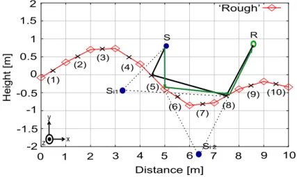
Let us explain the example of searched ray shown in Fig.2.4. First, we find the straight line from (5) to (8) which are in LOS. Second, we add the lines from S to (5) and from (8) to R, since S and (5) as well as (8) and R are in LOS. Thus, we obtain an approximate discrete ray from S to R through (5) and (8) as shown in black lines.

In order to obtain a more accurate ray, we can modify the discrete ray based on the imaging method. Si1 is an image source for first reflection point of line (5), and Si2 is an

image point of first reflection point for second reflection point of line (8). The final ray plotted in arrow line shows that the ray emitted from S is first diffracted at the right edge of line at (5) and next reflected by line (8), and finally it reaches R. We call this type of diffraction as an image diffraction, since it is associated with reflection and the reflection might be described as an emission from the image point with respect to the related line.

2 H e ig h t [m ] ‘Rough’ 1.5 1 0.5 0 -0.5 -1 -1.5 -2 0 1 2 3 4 5 6 7 8 9 10 Distance [m] (1) (2) (3) ₍₄₎ (5) (6) (7) (8) (9) (10) S R Si1 ™ ™ ™ ™ ™ ™ ™ ™ ™ ™ Si㸰 x y z

Figure 2.4: Example of searching the ray in case of LOS.

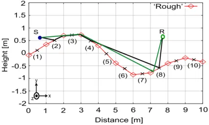
Let us explain another example of searched ray in Fig.2.5. First, we find a shortest path from (2) to (4) which are in NLOS and we also find a straight line (4) to (8) which are in LOS. Moreover, we add the straight line from S to (2) which are in LOS as well as the straight line from (8) to R which are also in LOS. Thus, we can draw an approximate discrete ray from S to R through (2), (3), (4) and (8). The discrete ray is shown by black lines.

In order to construct a more accurate ray, we modify the discrete ray so that the dis-tance from S to (8) may be minimum, and we apply the imaging method to the discrete ray from(4) to R through (8). The final modified ray is plotted in arrow lines in Fig.2.5. The ray from S to (8) constitutes a diffraction. We call it a source diffraction, because it is

associated with shadowing of the incident wave from source S through line (3). The ray from edge (3) to R through (8) is included into image diffraction.

We need to consider not only source diffraction but also image diffraction in order to genellary analyze scattered waves from an obstacle. However, in this analysis, we assume that the ray is constituted as image diffraction when it is in LOS, on the other hand, the ray is constituted as source diffraction in case of NLOS.

2 H e ig h t [m ] ‘Rough’ 1.5 1 0.5 0 -0.5 -1 -1.5 -2 0 1 2 3 4 5 6 7 8 9 10 Distance [m] (1) (2) (3) ₍₄₎ (5) (6) (7) (8) (9) (10) S R ™ ™ ™ ™ ™ ™ ™ ™ ™ ™ x y z

Figure 2.5: Example of searching the ray in case of NLOS.

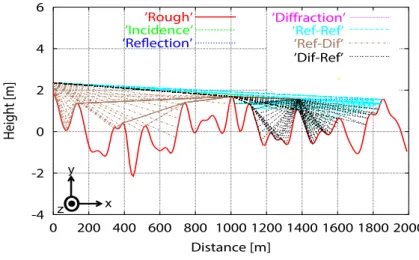
Figure 2.6 shows a numerical example of traced rays. The source is placed at x = 0[m] and 0.5[m] high above the rough surface, and the receiver is settled at x = 1, 380[m] and 0.5[m] high above the rough surface. In this numerical example, we have considered the rays up to the second order of reflections and diffractions, that is, incident, one-time reflection, two-time reflections and diffraction.

2.5

Field Computation

2.5.1

Incident and Reflected waves

Neglecting near fields, the electric field radiated from a small dipole antenna with input power Piis expressed in the following vector form [22]:

E0=

√

30GPi[(ur× p) × ur]Ψ(r) (2.14)

where r is a position vector from the source to a receiver and r =|r|. The direction of the unit vector ur= r/r is from the source to the receiver, and |ur× p| = D(ϕ) = sinϕ

2.5. Field Computation Chapter 2 -4 -2 0 2 4 6 0 200 400 600 800 1000 1200 1400 1600 1800 2000 He ight [m ] Distance [m] ’Rough’ ’Incidence’ ’Reflection’ ’Diffraction’ ’Ref-Ref’ ’Ref-Dif’ ’ ’Dif-Ref’ x y z

Figure 2.6: Examples of traced rays up to second scattered waves.

is the directivity of the small dipole antenna. The unit vector p is the direction of source antenna, and the source antenna gain is G. Moreover, the wave function is defined by

Ψ(r) = e− jκr

r , κ=ω

√

ε0µ0 (2.15)

whereκ is the wave number in the free space, and the time dependence ejωt is assumed. Figure 2.7 shows incident and reflected waves at a ground plane. We describe the incident wave as a source field since the wave radiates from a source, and we express the reflected wave as an image field since the wave behaves just as if it radiates from the image of the source. Received fields are expressed for E-wave and H-wave as follows:

Ez=Ψ(r0) + Rh(θ)Ψ(r) Hz=Ψ(r0) + Rv(θ)Ψ(r)

(2.16)

whereθ is an incident angle and r = r1+ r2. The reflection coefficients for horizontal and

vertical polarizations are given by [22]

Rh(θ) = cosθ− √ εc− sin2θ cosθ+√εc− sin2θ Rv(θ) =εccosθ− √ εc− sin2θ εccosθ+ √ εc− sin2θ εc=εr− j σ ωε0 (2.17)

S Si R θi r0 r1 r2 Plane Reflection r1 θr n S Si R θi r0 r1 r2 Plane Reflection r1 θr n

Figure 2.7: Incident and reflected waves.

2.5.2

Source and Image Diffraction Waves

Now we consider the source diffraction shown in Fig.2.8. We assume here that the elec-tromagnetic fields due to the source diffraction can be approximated by the Wiener-Hopf solution to the plane wave diffraction by a perfectly conducting semi-infinite half plane [23]. We omit the field expressions for H-wave for brevity, and the results are summarized as follows [11]: Ez= { E_zs− D(r,r0)Ψ(r) (RegionI) D(r, r0)Ψ(r) (RegionII) (2.18) where r = r1+ r2and the diffraction coefficient is given by

D(r, r0) = ejX 2

F(X ) X =√κ(r− r0) .

(2.19)

The complex type of Fresnel function is defined by [23]

F(X ) = e π 4j √ π ∫ _∞ X e− ju2du (X > 0) . (2.20) This function has the following analytical properties:

F(X ) = 1− F(−X) (X < 0) F(X )≃ e −π4j 2√πXe − jX2 (X≫ 1) . (2.21)

Finally we consider the image diffraction shown in Fig. 2.9 where the space is divided into three parts, Region I, II and III. In this case, we can summarize the image diffraction coefficients as follows:

2.5. Field Computation Chapter 2

Figure 2.8: Source diffraction by an edge.

R egion

R e gion

R egion

S

R

S

r

r12

r21

r

r

r

r

r

Ez=          Rh(θ)[D(r1, r0)Ψ(r1)− D(r2, r0)Ψ(r2)] (RgionI) Rh(θ)[Ψ(r0)− D(r1, r0)Ψ(r1)− D(r2, r0)Ψ(r2)] (RegionII) Rh(θ)[D(r2, r0)Ψ(r2)− D(r1, r0)Ψ(r1)] (RegionIII). (2.22)

where r0= r01+ r02, r1= r11+ r12and r2= r21+ r22. It should be noted that the

conven-tional reflection ray is included in the image diffraction ray in region II resulting in simpli-fication of the proposed DRTM. As mentioned in previous section, the image diffraction is employed when the source, receiver and the representative point at the discretized plate are all in LOS. In other cases, the source diffraction is used for the field computations.

2.5.3

Total Electric Fields

We have discussed the principle of DRTM algorithm to evaluate electric field approxi-mately. The electric field E at the receiver is formally expressed in the following dyadic and vector form:

E = N

∑

∏

∏

point given by Eq.(2.14). N is the total number of rays considered, M_ns is the number of times of source diffractions, and M_ni is the number of times of image diffractions of the

n-th ray. The distance of the n-th ray from source to receiver is given by

rn=

k=Mni+Msn

∑

k=0

rnk (n = 1, 2, . . . , N) (2.24)

where rnk is the k-th distance from a source or an image diffraction point to another.

In the numerical simulations, we select dielectric constants. As mentioned above, the reflection coefficients include the dielectric constants, but the diffraction coefficients are for perfect conductors and it dose not include those dielectric parameters. We have already analyzed the numerical accuracy by comparing with the experimental results, and we have demonstrated that the numerical solutions have a good accuracy [25].

2.6. Conclusion Chapter 2

2.6

Conclusion

We have reviewed the theory of DRTM in this chapter. Since we need various kinds of RRS when we analyze different kind of propagation environments for DRTM analysis, we have firstly described convolution method that numerically generates many kind of RRS characterised by two parameters, correlation length (cl) and height deviation (dv). We have secondary described the principle of discretization of rough surface and ray trac-ing, and finally we have described the theory of field computation. The general essence of DRTM is to discretize not only RRS but also ray tracing. The former helps saving computer memory and the latter simplify the ray searching algorithm resulting in saving computation time.

Chapter 3

Evaluation of DRTM

3.1

Introduction

We evaluate DRTM and apply to the EM wave scattering by a cylindrical conductor or by a conducting half-plane, and we check the accuracy of DRTM by comparing its results with rigorous analytical solutions. In case of a cylinder, its boundary is approximated in terms of piecewise-linear plates, and source and image rays are searched based on the approximated profile. The total scattered fields are given by superposing each scattered field related to each plate which is computed by use of the source and image diffraction coefficients obtained by the Fresnel function. In case of a half-plane, the total scattered fields are computed rigorously by using the Fresnel function.

In the former evaluation case, numerical results are compared with the rigorous so-lutions given by use of the Bessel and Hankel functions. In the latter evaluation case, numerical computations are performed to check the effect of diffraction points on the field distributions in shadow region. It is demonstrated that DRTM provides us a good convergence. We add explanations for two types of rigorous solutions in the end of this chapter; one is rigorous solution to the plane-wave diffraction by a conducting cylinder, and the other is rigorous solution to the plane-wave diffraction by a conducting half-plane .

3.2

Geometry of the Problem

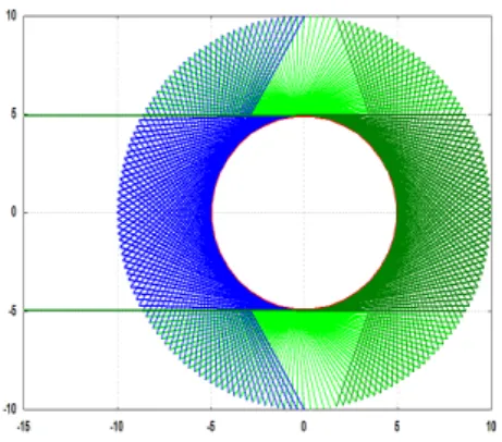
Figure 3.1 shows the geometry of the problem. Although the source is located at left hand side in this Figure, of course its location may be arbitrary. Originally the cross section of

3.3. Scattered Rays and Fields from the Cylinder Chapter 3

the cylinder is circle (red), but it is approximated in terms of piecewise-linear plates (blue) as shown in the Figure where the number of plates has been chosen as N = 8. Moreover, the radius of the cylinder is denoted by a, and the observation points are located on the circle (green) of radius r.

Geometry of the problem

Figure 3.1: Geometry of the problem.

In this chapter, we deal with scattering of the plane-wave by a perfectly conducting cylinder and a conducting half-plane. It is assumed that the structure is uniform in z-direction or two-dimensional (2D). We consider that the scattered field is defined by the total field (t) minus the source or incident field (s), that is, (E, H) = (Et, Ht)− (Es, Hs).

3.3

Scattered Rays and Fields from the Cylinder

Figure 3.2 shows some source diffraction rays from an edge at the upper side of the cylinder. The cylinder of radius 5[m] with its centre at the origin (x, y) = (0, 0) is divided into 36 plates, and the source is located at (x, y) = (−1000,0)[m]. Receiving points are located at the circle of radius 10[m], the operating frequency is selected as f = 300[MHz].

In addition to the source diffraction from the upper side, other rays caused by the source diffraction from a lower edge are included in Figure 3.3.

R=1000 r=10 a=5 f=300MHz ncy=36

step_degree=2 Nd=12

Figure 3.2: Source diffraction rays from an edge at the upper side.

R=1000 r=10 a=5 f=300MHz ncy=36

step_degree=2 Nd=12

3.3. Scattered Rays and Fields from the Cylinder Chapter 3

Figure 3.4 shows electric field distribution for E-wave computed by using only the source diffraction rays shown in Figure 3.3. In this case the fields are computed by

E_zsd= 2

∑

∑

where n = 1 and n = 2 correspond to source diffractions from the upper and lower edges, respectively. It should be noted that the minus source or incident field has been assumed in the shadow region. We explain rigorous solutions in section 3.6.

Figure 3.4: Source diffraction field (red) in comparison with the rigorous solution (green).

Figure 3.5 shows some image diffraction rays from one plate in the illuminated region; in this example, the image diffraction occurs at the 18-th plate corresponding to k = 18 in Eq.(3.2). The source point and the receiving points are chosen as the same as in Figure 3.2. Figure 3.6 shows image diffraction rays obtained by considering all the illuminated plates; in this example, the image diffractions occur at plates corresponding to k = 10 through

R=1000 r=10 a=5 f=300MHz ncy=36

step_degree=2 from plate 18

Figure 3.5: Image diffraction rays from one illuminated plate.

R=1000 r=10 a=5 f=300MHz ncy=36

step_degree=2 from illminated plates Nd=4

3.3. Scattered Rays and Fields from the Cylinder Chapter 3

Figure 3.7 shows electric field distribution for E-wave computed by summing up the results obtained by Eqs.(2.22) using only the image diffraction rays shown in Figure 3.6. These field computations are carried out by

E_zid = K

∑

∑

where K is the total number of illuminated plates.

Figure 3.7: Image diffraction field (red) in comparison with rigorous solution (green).

Finally we can obtain the total scattered fields by adding the source diffraction fields and the image diffraction fields as follows:

Ez= Ezsd+ Ezid

Hz= Hzsd+ Hzid .

Figure 3.8: Scattered E-wave obtained by DRTM with 36 plates (red) in comparison with rigorous solution (green).

Figure 3.9: Scattered H-wave obtained by DRTM with 36 plates (red) in comparison with the rigorous solution (green).

3.3. Scattered Rays and Fields from the Cylinder Chapter 3

Figure 3.8 and Figure 3.9 show scattered fields for E-wave and H-wave, respectively. It is shown that a better accuracy is achieved in case of E-wave than in case of H-wave.

3.4

Field Convergence and Number of Plates

Figure 3.10 shows scattered electric fields when the radius of the cylinder has been chosen as a = 10[m] and the observation points have been selected on the circle with radius

r = 20[m]. In this Figure, we have shown two types of cylinder discretizations for DRTM;

one is with 36 plates and the othr is with 72 plates, respectiely. It is shown that the DRTM solution with 72 plates exhibits a little more accurate numerical result than that with 36 plates.

Figure 3.10: Scattered E-wave obtained by DRTM with 36 (red) and 72 (blue) plates in comparison with rigorous solution (green).

Figure 3.11 shows scattered magnetic fields with the same parameters as the former example. In this Figure, we have shown two types of cylinder discretizations for DRTM; one is with 36 plates and the othr is with 72 plates, respectiely. It is shown that the DRTM solution with 72 plates exhibits a little more accurate numerical result than the other case with 36 plates. Moreover, it is demonstrated that results based on DRTM in case of H-wave show a poorer accuracy than those in case of E-H-wave.

3.4. Field Convergence and Number of Plates Chapter 3

Figure 3.11: Scattered H-wave obtained by DRTM with 36 (red) and 72 (blue) plates in comparison with rigorous solution (green).

Figure 3.12 shows root mean square errors of DRTM solutions in comparison with the rigorous solutions for the EM wave scattering by a conducting cylinder [27]. The pa-rameters used are such that the operating frequency is f = 300 [MHz] with corresponding wavelengthλ = 1 [m], the radius of conducting cylinder is a = 10 [m] with corresponding circumference ℓ = 62.8 [m] and the observation points are at r=20 [m] from the centre of the conducting cylinder. Moreover, the red line in this figure indicates E-polarized incidence and the blue line denotes H-polarized incidence.

It is demonstrated that the errors in case of H-wave are almost double of those in case of E-wave, and the error suddenly increases when the number of plates decreases into less than 30 plates. This means that we should keep the plate length∆x shorter than twice of the wave length. According to these numerical examples, the minimum error rate is about 5.9 % when the plate number is 140-220, when the plate length∆x is chosen as same as from 29 % to 45 % of the wave length, good accuracies are obtained.

And better accuracies are not achieved even if the boundary is divided into smaller pieces, in other words, the error gradually increases when the plate number becomes

more than 220 plates. It is shown from the numerical examples that the minimum error has been achieved for ∆x ≃λ. Thus, it is concluded that λ ≥ ∆x is required for field computations by use of DRTM.

a=5m r=10m S=(0,-1000) f=300MHz

Figure 3.12: Mean square errors of DRTM solutions compared with rigorous solutions.

3.5

Rigorous solutions

In this section, we explain two types of rigorous solutions which are noted through section 3.2 to 3.4.

3.5.1

Rigorous solution to the plane-wave diffraction by a conducting

cylinder

In this section we show the rigorous solutions in terms of Bessel and Hankel functions for the plane wave scattering by a perfectly conducting cylindrical rod [24]. Assuming that a plane wave e− jκ(xcosθi+y sinθi) _{with incident angle}θ

3.5. Rigorous solutions Chapter 3

cylinder of radius a, we have the rigorous solution for the scattered E-wave as follows:

Ez=− ∞

∑

where Jn(x) is the Bessel function of the n− th order, and Hn(2)(x) is the second kind

of Hankel function of the n− th order. It should be noted that we have employed the polar coordinates (r,Θ) having the relations with the Cartesian coordinates (x,y) such as

x = r cosΘ and y = r sinΘ.

On the other hand we have the rigorous solution for the scattered H-wave as follows:

Hz=− ∞

∑

where the prime of the Bessel or the Hankel function denotes the derivative of the function with respect to their argument.

3.5.2

Rigorous solution to the plane-wave diffraction by a conducting

half-plane

It is well-known that the plane wave diffraction by a conducting half plane can be solved rigorously by use of the Winer-Hopf technique [23]. The results are compactly expressed in terms of the complex type of Fresnel function defined in Eq.(2.21). Since the Winer-Hopf solutions to the plane wave diffraction by a conducting half-plane are considered to be the basis of the DRTM, we summarize the final results in the following.

The geometry of the problem is shown in Figure 5.1 where the half-plane is uniform in z-direction (two-dimensional) and we select the edge point as (A = B = 0) so that the edge coincides with the origin. Then we have the field expression for E-wave with the reflection coefficient Re=−1 as follows:

E_zt(x, y) =            Ds(Xs)e− jκr+ ReDi(Xi)e− jκr (θi<Θ <π) e− jκr cos(Θ−θi)− D s(Xs)e− jκr+ ReDi(Xi)e− jκr (−θi<Θ <θi) e− jκr cos(Θ−θi)− D s(Xs)e− jκr+ Ree− jκr cos(Θ+θi) −Re_D i(Xi)e− jκr (−π<Θ <θi) (3.6)

Moreover, we have the field expression for H-wave with the reflection coefficient Rh= 1 as follows: H_zt(x, y) =            Ds(Xs)e− jκr+ RhDi(Xi)e− jκr (θi<Θ <π) e− jκr cos(Θθi − D_s(X_s)e− jκr+ RhD_i(X_i)e− jκr (−θ_i<Θ <θ_i) e− jκr cos(Θ−θi)− D s(Xs)e− jκr+ Rhe− jκr cos(Θ+θi) −Rh_D i(Xi)e− jκr (−π<Θ <θi) (3.7) where the diffraction functions are given by

Ds(Xs) = ejX 2 s_F(X s) Di(Xi) = ejX 2 i_F(X i) (3.8) and Xs= √ κr[1− cos(Θ −θi)] Xi= √ κr[1− cos(Θ +θi)] . (3.9)

3.6

Conclusion

We have evaluated DRTM, applying the source and image diffraction coefficients to the EM wave scattering by a cylindrical conductor to check the accuracy of DRTM since we have rigorous analytical solutions to be compared with. We also evaluate DRTM with the plane wave diffraction by a conducting half-plane since the scattered field for this problem can be computed rigorously by using the Fresnel function.

Numerical examples have been given for the source and image diffraction rays as well as the field distributions. Accuracy of DRTM has been discussed in comparison with the rigorous solutions focussing on the number of plates discretizing the cylinder. It has been demonstrated that DRTM has a good accuracy and there exists an appropriate optimal number for the cylinder discretization.

Chapter 4

Application to Long Distance

Propagation

4.1

Introduction

In this chapter, we apply DRTM to the long distance propagation analysis of terrestrial digital TV waves and we apply GIS to obtain surface profile data. In Fukuoka area, the terrestrial digital TV has been broadcasting from Fukuoka tower which is the highest buildings in the local area and located at the central part of Fukuoka city. However, the city is surrounded by mountains except for the northern part of sea side, therefore there exist some blind zones where the base stations cannot cover. As a result, relay stations should be constructed to overcome the blind zone problems. In this chapter, we estimate electric field distributions from three sources; main station at Fukuoka tower and two relay stations at Mt. Kaya and Fukae area.

We have two steps of field estimation procedure in this chapter. First, we apply the GIS system to obtain surface profile data. Second, we apply the DRTM to compute electric field distributions along the straight line between the two points. By numerical results of the DRTM, we have recognized the performance of existing two relay stations for those areas. The relay station at the top of Mt. Kaya covers Maebaru area which is in the west direction from Fukuoka city. The relay station in Fukae can cover only a small area due to so little input power. We have confirmed that the DRTM has a good performance to estimate EM fields for long distance propagation.

Figure 4.1: Incident rays in the region of LOS.

Figure 4.2: Diffraction rays in the region of NLOS.

4.2

Incident Rays and Diffraction Rays

Figure 4.1 shows an example of incident rays in the region of LOS corresponding to the 0th order rays. Figure 4.2 shows an example of diffraction rays in the region of NLOS corresponding to the 1st order rays. Reflected rays of the 1st order and reflected and/or diffracted rays of the second order are omitted in these figures. As we can see here, the incident rays are dominated in open area or LOS region as shown in Figure 4.1, and the diffraction rays are dominated in shadow area or NLOS region as shown in Figure 4.2.

4.3. Import of Terrain Profile Data Chapter 4

4.3

Import of Terrain Profile Data

We introduce GIS to import the terrain profile data. The GIS is a integrated system for analyzing and displaying all forms of geographically referenced information that allows us to view, understand and visualize data in many ways that reveal relationships in the form of maps and the information. The GIS helps our methods of collecting data and carrying out the propagation analysis.

The proposed procedure for importing terrain data is composed of two steps. The first step is to import a sampling data for the terrain profile, and second one is to convert the data to continuous numerical terrain data.

4.3.1

Import of sampling data

We can obtain the sampling data for the terrain profile between two designated points by applying the GIS. In Figure 4.3 a screen shot of the system is shown, we can get the sampling data for the terrain profile between the two designated points. In this Figure, one point is at Fukuoka tower and the other point is at Maebaru beyond Mt. Kaya. After selecting two points, we have the sampling data for the required terrain profile as shown in Figure 4.4. The sampling data cannot be straightforwardly applied to DRTM, so that we have to convert the data to a continuous numerical data. Thus we can import the numerical data{xm, ym} (m = 0,1,2,··· ,M) as a text file.

Mt. Kaya

Fukae area

Figure 4.4: Sampling data for a required terrain profile.

4.3.2

Regeneration of a continuous terrain profile

We assume that the interval of the numerical data in x-direction to be Dx, that is, xm=

mDx (m = 0, 1, 2, . . . , M). Then we can introduce an approximate height function for the

terrain profile data regeneration as follows:

f (x) = m=M

∑

Eq.4.1 provides an approximate but continuous terrain profile, and we can easily apply the height data obtained by this equation to a DRTM simulation. Figure 4.5 shows an approximated terrain profile regenerated by Eq.4.1. It is demonstrated that the regener-ated numerical data illustrregener-ated in Figure 4.5 is in good agreement with the sampling data illustrated in Figure 4.4.

4.4

DRTM simulations for field distributions

Figure 4.6 shows the geometry of the problem. In the present DRTM simulations, we have assumed that there exists a sea surface in the region from x = 3km to 7km and other regions are occupied by a dry ground surface. The antenna of main station is located on Fukuoka tower at x = 0m and y = 234m, and the relay station transmitter is located at 5m above the top of Mt. Kaya (365m). In the numerical simulations, we have assumed that the observational points are 5m above the sea or ground surface. Frequency is selected as f = 527.0MHz which is the operating frequency of NHK terrain digital broadcasting

4.4. DRTM simulations for field distributions Chapter 4 -50 0 50 100 150 200 250 300 350 400 0 5000 10000 15000 20000 He ig ht [m ] Distance [m] ’Terrain’

Figure 4.5: Regenerated curve for the terrain profile.

service. Input powers are 3KW and 30W at the Fukuoka tower and Mt. Kaya, respectively.

Source1

(Fukuoka Tower)

Source2 (Mt. Kaya)

A

Sea surface Sea surface

Figure 4.6: Geometry of the problem.

Figs.4.7 and 4.8 show the electric field intensities radiated from the main station at Fukuoka tower and the relay station at Mt. Kaya, respectively. It is shown in Figure 4.7 that the field intensity radiated from the main station is decaying apart from the station, but it keeps relatively high level due to the high input power (3KW ). Because of the shadowing effect of a mountain near at x = 19Km, however, there exists a blind zone A where electric field intensities are below −60dB. On the other hand, Figure 4.8 shows

that the field intensities radiated from the relay station are much higher than−60dB at the region A, and thus the relay station covers the blind zone effectively.

-80 -70 -60 -50 -40 -30 -20 -10 0 10 0 5000 10000 15000 20000 Fi eld Intensity [dB ] Distance [m] ’Field intensity’ (Fukuoka Tower) Blind Zone A

Figure 4.7: Intensity of radio wave emitted from the main station at the Fukuoka tower.

-80 -70 -60 -50 -40 -30 -20 -10 0 10 0 5000 10000 15000 20000 Fi eld Intensity [dB ] Distance [m] ’Field intensity’ (Mt. Kaya) A Blind Zone

Figure 4.8: Intensity of radio wave emitted from the relay station at Mt. Kaya.

In Figure 4.9, we have compared the field distribution radiated from the main station with that from the relay station. In Figure 4.10, we have shown only the maximum part of the two field distributions radiated from the main and relay stations. It is well demon-strated that the field intensity level in Figure 4.10 is much higher than −60dB almost everywhere in the range 0 < x < 25km.

Figure 4.11 shows the incident rays emitted from the main station. Figure 4.12 shows field distributions of the radio wave radiated from the main station. It is shown that

4.4. DRTM simulations for field distributions Chapter 4 -80 -70 -60 -50 -40 -30 -20 -10 0 10 0 5000 10000 15000 20000 Fi eld Intensity [dB ] Distance [m] ’Fukuoka Tower’ ’Mt. Kaya’ Blind Zone A

Figure 4.9: Intensities of radio waves emitted from the main and relay stations.

-80 -70 -60 -50 -40 -30 -20 -10 0 10 0 5000 10000 15000 20000 Fi eld Intensity [dB ] Distance [m] ’Field intensity’ Blind Zone A

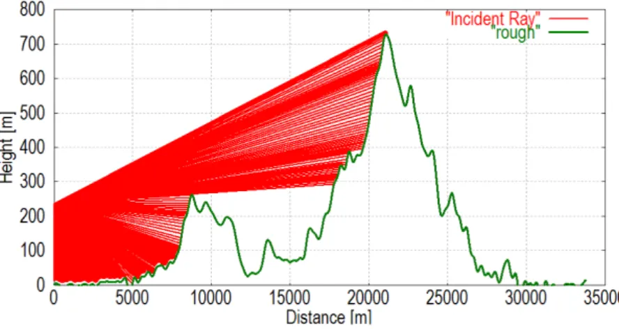
Figure 4.10: Maximum part of the two radio waves emitted from the main and relay stations.

incident rays reach the top of Mt. Kaya where the relay station is located, and some degree of field decays are observed in the shadow regions.

Figure 4.13 shows incident rays emitted from the relay station at Mt. Kaya. Figure 4.14 shows field distributions of the radio wave radiated from the relay station. It is shown that some degree of field decays are observed in the shadow region. Reflected waves from the sea surface are also observed between 3km < x < 7Km. Comparison of Figure 4.12 with Figure 4.14 reveals clearly that the blind zone of the main station is cancelled by the radiation from the relay station.

-50 0 50 100 150 200 250 300 350 400 0 5000 10000 15000 20000 25000 He ig ht [m ] Distance [m] ’Rough’

’Incident ray from Tower’

Figure 4.11: Incidence rays in LOS from the main station at the Fukuoka tower.

Figure 4.12: 2D field distributions from the main station at the Fukuoka tower.

Next, we consider other area in western part of Fukuoka. Fukae area is located at southern part of Mt. Kaya. Figures 4.15 and 4.16 show geometry of the problem and field intensities radiated from the Fukuoka tower. In these Figures, Fukae area is located at near x=20km. Because of the shadowing effect of mountain near x=10km, there exist a blind zone in Fukae area. To overcome this problem, the relay station at Mt. Kaya plays an important role.

4.4. DRTM simulations for field distributions Chapter 4 -50 0 50 100 150 200 250 300 350 400 0 5000 10000 15000 20000 He ig ht [m ] Distance [m] ’Terrain’

’Incident rays from Mt. Kaya’

Figure 4.13: Incident rays in LOS from the relay station at Mt. Kaya.

-50 0 50 100 150 200 250 300 0 5000 10000 15000 20000 He ig ht [m ] Distance [m] ’Terrain’ ’Observe’ Fukae area Source1 (Fukuoka Tower)

Figure 4.15: Geometry of the problem (from Fukuoka tower to Fukae area).

-80 -70 -60 -50 -40 -30 -20 -10 0 10 0 5000 10000 15000 20000 Fi eld Intensity [dB ] Distance [m] ’Field intensity’ (Fukuoka Tower) Blind Zone Fukae area

Figure 4.14: 2D field distributions radiated from the relay station at Mt. Kaya.

Figures 4.17 and 4.18 show geometry of the problem and field intensities radiated from the relay station at Mt. Kaya. It is shown that even though the field intensities from Mt. Kaya keeps high level, there exists a new blind zone beyond the hills. Therefore, another relay station is required to overcome the new blind zone.

4.4. DRTM simulations for field distributions Chapter 4 -50 0 50 100 150 200 250 300 350 400 0 1000 2000 3000 4000 5000 6000 7000 8000 He ig ht [m ] Distance [m] ’Terrain’ ’Observe’ Source2 (Mt. Kaya) Fukae area

Figure 4.17: Geometry of the problem (from Mt. Kaya to Fukae area).

-80 -70 -60 -50 -40 -30 -20 -10 0 10 0 1000 2000 3000 4000 5000 6000 7000 8000 Fi eld Intensity [dB ] Distance [m] ’Field intensity’ (Mt. Kaya) Fukae area Blind Zone

Figure 4.18: Intensity of radio wave emitted from the relay station at Mt. Kaya.

Figures 4.19 and 4.20 show geometry of the problem and field intensities radiated from a small relay station at Fukae. It is shown that the new blind zone is cancelled by the small relay station with the input power of which is only 50[mW ]. As a result, it is found that the blind zone from the relay station can be cancelled by another relay station installed with so small input power.

0 20 40 60 80 100 120 0 500 1000 1500 2000 He ig ht [m ] Distance [m] ’Terrain’ ’Observe’ Source3 (Fukae)

Figure 4.19: Geometry of the problem (Fukae area).

-80 -70 -60 -50 -40 -30 -20 -10 0 10 0 500 1000 1500 2000 Fi eld Intensity [dB ] Distance [m] ’Field intensity’ (Fukae) Blind Zone Blind Zone (from Mt. Kaya)

Figure 4.20: Intensity of radio wave emitted from a small relay station at Fukae area.

Results of numerical simulations shown so far are summarized as follows. Even though the main station’s input power level is high, the electric field intensities in the NLOS region are generally small, where there may exist some blind zones. However, these blind zones can be clearly and effectively cancelled by the relay station installed at