An Optimization Problem in a Finite Markov Chain Applied to Solid Particle Mixing

(1)

Journal of the Operations Research Society of Japan

Vol. 26, No. 2, June 1983

AN OPTIMIZATION PROBLEM IN A FINITE MARKOV CHAIN

APPLIED TO SOLID PARTICLE MIXING

Keisuke Uchimura Tadashi Yoshizawa

Yamanashi University Yamanashi University

Kenichi Shimura

Yamanashi University

(Received January 20,1981; Final February 25,1983)

Abstract Consider a Markov chain with n states and a symmetric tridiagonal transition probability matrix P.

Let C be a class of vectors I p(O) I such that half the elements of p(O) are zero and another half are 1. The problem is to find the vector p(O) in C such that the value IIp(Or -p(oo)11 is the minimum for any large nonnegative integer N, where p(oo)

=

(1/2,1/2, ... , 1/2) and p(oo) is Galled a stationary concentration vector. The solution is stated as follows. The optimal vectors in a sense defined in this paper are of the form _{(PO,Pl'··· ,Pn-l)}which satisfy the following conditions: Pk = P3-k' Pk = P4gtk for 0:'£ k :'£ 3 and 0:'£ g:'£ 1m-2_1, where n = 2m (m ~ 2). The optimal vectors can be represented as repetition of 0110 or 1001.

This problem was related to models for mixing process of particulate solids. The optimal solutions have been conjectured through the computer simulation conducted by Akao et al. The objective of this paper is to support the mathematical background for their experimental results and to show an interesting property of Markov chains.

1. Introduction

The problem formulated and solved in this paper is to find an optimal initial distribution for Markov chains with some specific transition proba-bility matrix. An initial distribution is said to be optimal if the speed of convergence from the initial distribution to the stationary one is the maximal.

This problem was first suggested by Akao, who has proposed a significant approach to analyse mixing processes of solid particles.

Mixing process in a conventional solids mixer is governed mainly by two basic mechanisms, convection and diffusion. In fact, fairly regular determi-nistic bulk flow of particles and very irregular stochastic movement of individual particles will be easily observed typically i f the two kinds of

85

(2)

86 K. Uchimura, T. Y oshizawa and K. Shimura

particles are mixed by a horizontal rotating drum mixer, which is probably one of the simplest types of conventional solids mixer used 1n various indus-tries. However, real motions are extremely complicated and depend on the shape, density and other physical characteristic of particles as well as types of mixers. Mixing is one of the difficult problems to analyse in chemical engineering.

Akao et al. (1,4] regard mixing process as a synthesized one with two independent operational units which correspond to convention and diffusion. They have proposed a probabilistic branching model for diffusive unit, and studied for convection unit optimal constitution of strata fed to the follow-ing diffusive unit. The problems of constitution of strata may be observed, for examples, at strata of cokes and ores in blast furnace in iron-works. If we find the optimal constitution of strata, we can considerably shorten the time required for the mixing.

Numerical and experimental simulation studies on mixing of particulate solids have been reported in Akao et al. (1, 3, 4]. The details of further results and of their applicability to the design of practical mixers will be published in Akao et al. [2]. Concerning the problem solved here, the optimal solutions has been conjectured through their extensive computer simulation [2, 3].

The objective of the present paper is to support the mathematical back-ground for their experimental results. We can regard the constitution of strata as initial distributions for Markov chains. Hence if we can find the optimal initial distribution, we can get the-optimal constitution of strata accordingly.

In the second section the probability branching model mixer and the structure of the transition probability matrix will be described on the basis of a Markov chain. The optimization problem to be solved here will be formulated in the third section, where eigenvalues and eigenvectors of the transition probability matrix will be also derived, showing a numerical example. In the fourth section, an algebraic proof of the theorem concerning the optimality will be given. In the fifth section, several modifications of the Markov chain model will be discussed. The approach to this problem will be interesting for readers of this journal since applications of Markov chains are broad in the field of Operation Research.

(3)

A Finite Markov Chain

diffusive mixing processes as shown in r'ig. 1, which is a revised version of Fig. 7 in [4], The upper parts and the central parts of the mixer represent stratified feeders which play a role of convection and a probabilistic branching model mixer which realizes diffusion, respectively. The lower parts are simply receivers of the mixture.

stage 0 stage 1 stage 2 stage 3 stage 4 stage 5

8

0

•

0 0 0 0

0 0 0

0 0°0

0 0°

0

0 0 0 0

0 0 0

0 0 0 0

0 0 0

° 0 °

0 0 0 0 0

0 0

0 0 0

0

0 0 0

0

0 0 0

2 3 4 13 14 15

Fig. 1 A stratified feeding mixer and a probabilistic branching model mixer.

0 I

_~ Q) '"0 Q) Q) 4-< '"0 Q) oM 4-< oM _...., <1l ~ ...., rJ)

0

t

~

0

Q) ~ oM s Q)

0

_oM:> rJ) :l 4-<

0

4-< oM '"0

0

t

~ Q) :> oM Q) () Q) :....

1

16 87

(4)

88 K. Uchimura. T. Yoshizawa and K. Shimura

This paper deals with the mixture of only two kinds of homogeneous solid particles, whose total concentration is fixed to be one to one. Two kinds of particles are classified into

°

(white) and 1 (black) here for convenience. Each feeder supplies particles either of type

°

or 1, so that the combination of feeders is represented by a vector with the elements of

°

and 1. The vectors are named "feeding vectors". In Fig. 1, the feeding vector is expressed as a IOW vector (1,1,0,0,1,1,0,0,1,1,0,0,1,1,0,0).

The probabilistic branching model mixer depicted in Fig. 1 is an inclined board with rows of hexagonal blocks set apart by a small distance. Particles with a diameter of slightly less than the distance between the blocks are dropped from the feeders. They are allowed to run down between the hexagonal blocks and are collected in the receivers at the bottom of the board. On their way down, particles are assumed to be independent of each other, that is, no interference exists. The rows numbered by every other rows in Fig. 1 are called stages, at which the locations between hexagonal blocks are called cells. The number of cells is denoted by n. In Fig. 1, each stage has 16 cells.

Motions of particles in the probabilistic branching model in [4] was considered a Markov chain as follows: the cells at each stage constitute a state space; the transition probability P .. from the state i to the state

~J

j is the probability that a particle which is located on the i-th cell at any stage moves to the j-th cell at the next stage; the transition proba-bility matrix with the elements P .. ' s is of the form

~J (2.1) P 3/4 1/4

o

1/4 1/2 1/4

o

1/'~ 1/2 1/4 1/4 3/4

where P is a real symmetric tridiagonal matrix. The quantities of P .. 's

~J

can be evaluated under the assumptions that a particle at any row branches with equal probability of 1/2 except at the walls, and both side walls are reflective.

Let us denote a row vector of an initial distribution by

n(O)

in the case that only one particle is dropped. The element

TI.(O)

of

n(O)

means

~

the probability that the particle is supplied from the i-th feeder (i=1, 2,

(5)

A Finite Mal'kov Chain

(2.2) IT(N)

=

IT(O)pN

and that the stationary distribution IT(OCo) exists and is equal to (l/n, l/n,

1 /n). Note that the element IT. (N) of IT(N) represents the probability that:

~

the dropping particle passes the i-th cell at stage N.

Suppose that many particles are supplied continuously and that the number of one kind of particles, e.g. black ones, follows the initial dis--tribution IT(O). The quantity (n/2)IT(N) can be interpreted as the expected concentration vector whose element represents the concentration ratio of black particles at each cell after N stages.

A feeding vector with 0-1 elements is denoted by p(O). Since p(O) 1.8

nothing but an initial concentration vector, p(N) which is defined by

(2.3) p(N) p(O)p , N

is equivalent to the expected concentration vector mentioned above, i.e.

(2.4) p(N)

=

(n/2)IT(N).

Then, we obtain

(2.5) p(co) (n/2)IT(oo)

(1/2, 1/2, •.. , 1/2)

89

as a stationary concentration vector, when the number of stages N approaches to infinity. The mixture with this stationary concentration vector is called "complete".

Akao et al. [2] have shown that the speed of convergence of P(N) to

p(co) greatly depends on the feeding vectors. Moreover, they have conjectured the feeding vectors which are optimal in a sense. For example, the feeding vector (1,0,0,1,1,0,0,1,1,0,0,1,1,0,0,1) is conjectured to be optimal for the case n=16 in Fig. 1. Note that the distinction of

°

and 1 in feeding vectors is not essential, since the same discussion as above is possible for the concentrat.ion of white particles instead of black ones.

3. Statement of the Problem and an example

Consider a finite Markov chain with n states and with the transition probability matrix P of the form

(6)

90 K. Uchimura, T. Yoshizawa and K. Shimura p+q q (3.1) p

o

q p q

_o

q p q q p+q

where P is a real symmetric tridiagonal matrix of size nxn, and

(3.2) 1 > P ~ 1/2 , and

(3.3) P -I- 2q

=

1.

The case in which p is 1/2 is reduced to the model with the transition probability matrix (2.1) described in the previous section, while the other cases in which p is greater than 1/2 may be physically interpreted as models in which some interferences among particles occur. If the condition (3.2) is satisfied, P is positive definite and has the distinct eigenvalues as will be shown in Appendix A. The condition (3.3) shows that the sum of the elements of each row in P is equal to 1.

The problem to be solved here is to find a feeding vector p(o) such that the expected concentration vector p(N) defined by (2.3) converges to the stationary concentration vector p(oo) as f~t as possible. The speed of convergence may be measured with the smallest value of N that satisfied the condition;

(3.4) 11 p(N) - p(oo)1! E < E

for a sufficiently small E, where 11.11 E denotes Euclidean norm about vectors. Now, we denote the eigenvalues and the corresponding eigenvectors of the transition probability matrix P by A. and

U.

(j=0, 1, " ' , n-1) re

spec-] ]

tively, i.e.

(3.5)

where A. I S are arranged as

]

j=o,

1, " ' , n-l,

(3.6)

_A

o

>

Al

> ••• >

A

n-

1

>

° ,

and

ii .'

s are assumed to be normalized as

]

(3.7) t- -u.u.

(7)

so that they are orthonormal. Note that: u. is a column vector, while peN)

~

is a row vector, and that t means transposition of a vector or a matrix, hereafter.

I t is well known that the maximum eigenvalue of the probability matrix

p is 1, and that p is decomposable to the form

(3.8)

n-l

P L A

.u

tu .'

j=O ] ] ]

91

From the above facts and the orthonormality of the

u

.'s, we can easily obtain

]

(3.9)

Therefore, the expected concentration vector peN) of (2.3) is expressed as

n-l _N _- _{; ..} -LA. (p (0) u .) - u . j=O ] ] ] (3.10) n-l t- N

t-a

O

U

o

+ j=l ] ]

L A.a.

U., ]

where a. is the inner product of p(O) and u i.e.,

] j'

(3.11) a. = p(O)ii .,

] ]

o

~ j ~ n-l.

Since the maximal eigenvalue AO is 1 and the other Aj'S are less than 1, we obtain

(3.12)

From (3.10) and (3.12), inequality (3.4) can be written as

(3.13) 11 peN) - p(oo)1I E

=

11 n-l L

A.a .

N t -u.1I E

j=l ] ] ]

Then, let us define the quantity a(N) as

(3.14) a(N) = 1 ₁n-1 L A N .a. t-u. 11

In

1/2

.

j=1 ] ] ] E

It is easily observed that a(N) will large N if a

1 is not equal to zero.

2N 2 be dominated by

Al

a

1 for a sufficiently

A~Na~

is said to be the principal term

(8)

92 K. Uchimura. T. Yoshizawa arui K. Shimura

of O(N) if a

k is the first nonzero factor in (3.14), that is a 1

=

a₂

= ••• =

a_k-₁

= 0,

and a_k '" O.

Consider a class C of feeding vectors

{p(O)}

such that half the elements of

p(O)

are zero and another half are 1. We order the vectors in C as follows. For any P1 and P2 in C, let

(3.15) _P1u₁ _P1u_{k - 1} 0, P₁u

k

'"

0 and (3.16) P₂u₁

...

= _P2u_s-₁ 0, P2u_s

_{'" O.}

Then, (3.17) P₁_{;;;; P2}if and only i f k > 5 or both k

=

5 and

Ip

1

u

k

l

;;;;

Ip

2

u

k

l

hold.

The minimal elements are called the optimal feeding vectors. It is clear that if

p(O)

is an optimal feeding vector, the smallest integer

N

satisfying the condition (3.4) with

p(O)

is the smallest of all integers with vectors in C.

Problem

Find the optimal feeding vectors in C.

Note that the feeding vector

p(O)

is regard to be proportioned to an initial distribution n(O) as mentioned in the previous section, so that this problem can be stated concerning initial distribution instead of feeding vectors.

Now, let us show the eigenvalues and eigenvectors of the transition probability matrix P of (3 .. 1). The d:tails of their derivation will be de-scribed in Appendix A. The eigenvalues of P are given by

(3.18) where (3.19)

A .

_]

=

p + y _jq _, y. = 2cos{jrr/n), ]

o ;;;;

j ;;;; n-l,

o ;;;;

j ;;;; n-l.

The corresponding eigenvectors u

j ' whose elements are denoted by uj,k

(0 ;;;; k ;;;; n-1), are expressed as

(3.20) Uj,k

= cos«2k+1)jrr/2n),

j=O, 1, ... , n-l.

Note that

(3.21) II . = U . / (n /2) 1/2 ,

] ] j ~ 1.

It is worthy of noticE! that the eigenvectors do not depend on p and q.

Since y .'s are distinct and

(9)

1 y.1

~ 2,

]

j=O, 1, .•. , n-1,

the eigenvalues of P are distinct and positive i f p and q satisfy (3.2) and (3.3) • Note that AO is equal to 1 as well known, and that

t

U

o

= ( 1, 1, ••. , 1). Thus, we know from (3.11),

a = n 1/2/2

o

and

for any p(O) which belongs to the class restricted in the problem.

The numbe'(" of entries of the class {p(O)} is finite for any fixed n,

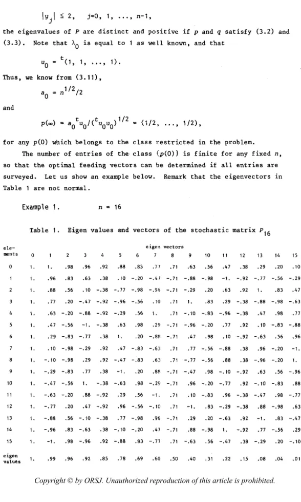
so that the optimal feeding vectors can be determined if all entries are surveyed. Let us show an example below. Remark that the eigenvectors in Table 1 are not normal.

Example 1.

n 16

Table 1. Eigen values and vectors of the stochastic matrix P 16

ele- eigen vectors

ments _o 3 4 5 6 8 9 10 11 12 13 14 93 15

o

1. 1. .98 .96 .92 .88 .83 .71 .71 .63 .56 .47 .38 .29 .20 .10 2 3 4 5 6 1. .96 .83 .63 .38 .10 -.20 -.41 -.71 -.88 -.98 -1. -.92 -.77 -.56 -.29 1. .88 .56 .10 -.38 -.77 -.98 -.96 -.71 -.29 .20 .63 .92 1. .83 .47 1. .77 .20 -.47 -.92 -.96 -.56 .10 .71 1. .83 .29 -.38 -.88 -.98 -.63 1. .63 -.20 -.88 -.92 -.29 .56 1. .71 -.10 -.83 -.96 -.38 .47 .98 .77 1. .47 -.56 -1. -.38 .63 .98 .29 -.71 -.96 -.20 .77 .92 .10 -.83 -.88 1. .29 -.83 -.77 .38 1. .20 -.88 -.71 .47 .98 .10 -.92 -.63 .56 .96 1. .10 -.98 -.29 .92 .47 -.83 -.6:1 .71 .77 -.56 -.88 .38 .96 -.20 -1. 8 1. -.10 -.98 .29 .92 -.47 -.83 .63 .71 -.77 -.56 .88 .38 -.96 -.20 1. 9 1. -.29 -.83 .77 .38 -1. .20 .88 -.71 -.47 .98 -.10 -.92 .63 .56 -.96 10 1. -.47 -.56 1. -.38 -.63 .98 -.29 -.71 .96 -.20 -.77 .92 -.10 -.83 .88 11 1. -.63 -.20 .88 -.92 .29 .56 -1. .71 .10 -.83 .96 -.38 -.47 .98 -.77 12 I. -.77 .20 .47 -.92 .96 -.56 -.10 .71 -1. .83 -.29 -.38 .88 -.98 .63 13 1. -.88 .56 -.10 -.38 .77 -.98 .96 -.71 .29 .20 -.63 .92 -1. .83 -.47 14 1. -.96 .83 -.63 .38 -.10 -.20 .47 -.71 .88 -.98 1. -.92 .77 -.56 .29 15 eigen values 1. 1. -1. .98 -.96 .92 -.88 .83 -.77 .71 -.63 .56 -.47 .38 -.29 .20 -.10 .99 .96 .92 .85 .78 .69 .60 .50 .40 .31 .22 .15 .08 .04 .01

(10)

94 K. Uchimura, T. Yoshizawa and K. Shimura

We have computed the integer k such that a

k is the first nonzero factor

in (3.14) and the value a},: for fifteen feeding vectors of size 16. Further we have evaluated the mini.mal integer NO that satisfies the inequality

(3.22)

for each feeding vector by direct computation.

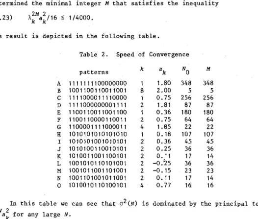
Besides we have determined another integer M for each feeding vector as follows. Let

A~Na~

be the principal term of a(N) for the vector. We have determined the minimal inl:eger M that satisfies the inequality

0.23)

A~Ma~/16

:s

1/4000.

The result is depicted in the following table.

Table 2. Speed of Convergence

patterns k ak NO M A 1111111100000000 1 1.80 348 348 B 1001100110011001 8 2.00 5 5 C 1111000011110000 1 0.75 256 256 D 1111000000001111 2 1.81 87 87 E 1100110011001100 1 0.36 180 180 F 1100110000110011 2 0.75 64 64 G 1100001111000011 4 1.85 22 22 H 1010101010101010 1 0.18 107 107 I 1010101001010101 2 0.36 45 45 J 1010100110010101 2 0.25 36 36 K 1010011001100101 2 O. '1 17 14 L 1001010110101001 2

-ohs

36 36 M 1001011001101001 2 -0.15 23 23 N 1001101001011001 2 0.11 17 14 0 1010010110100101 4 0.77 16 16

In this table we can see that a2(N) is dominated by the principal term 2N 2

Ak

a_k for any large N.

Here we explain the reason for using the value 1/4000 in (3.22) and 0.23).

Akao et al. compared the speed of convergence among the fifteen feeding vectors by computer simulation. Although a(N) becomes zero in the complete mixed state, the simulation results are acompanied by the error of the simple random sampling. The value a 2 of the error is evaluated to be

r 2

a

=p(l-p)/k

r

based on the binomial distribution, where k is the number of particles fed at each cell (See, [2]). The criterion of convergence can be determined as

i(N):sa 2/10

(11)

from the convention which is practically employed in the field of sampling. In their simulation 100 particles were fed.

In order to compare our result with theirs. we chose the value 1/4000 and evaluated the integers NO and M.

In Table 2 we see the fact that the speed of convergence of the pattern

B is the faste,st. which accords with the result of the computer simulation stated in [2].

4. Optimal Solutions in the case that n

=

2m

In this section. the theorem which gives the optimal solutions of the problem will be proved. where n

=

2m.

Theorem.

Where n

=

2m (m ~ 2). the optimal feeding vectors of the

problem stated in the previous section are the feeding vectors of the form (PO' P₁• •••• P

n-1) which satisfy the following condition cm_2;

o :;;

k :;; 3.

Representing the optimal vector (PO' P

1, •••• Pn-1) as a string POP1 •••••

P

n-1• we have

where Ci

i = Cij._1*Cii_1, and CiO = 0110 (or 1001) (the symbol

*

denotes a

concatenation product of two strings).

To prove the theorem we need some preparation. Recall that from (3.20) we have

U. L

=

cos «2k+l)jn/2n).

J.'"

Let l;

= exp

(2ni/4n). Clearly l; is a primitive 4n-th root of unity. Then

we have

rj (2k+l) -j(2k+l)

2u . k

=

~ + l; ,

J,

o :::;

k :;; n-l ,

since l; cos(2n/4n) + isin(2n/4n). Note that

2l11'1·2

l; = 1 and l; 2m+l = -1.

95

(12)

t -1 3 -3 2n-1 -(2n-1)

Note that 2u

1

=

(r;;+r;; ,~; +r;; , ••• , r;; +r;; ) and each element of

p(O) is

1

or

O.

Lemma 1. The equality,

(4.1) 0,

where each c

k is in the rational number field Q, is valid if and only if

C for all k

=

0,1, ••• , 2m-1.

2m_1_k

P

_roo:

f _Letn. _~_m+2( ) _x _{be t e}h 2m+2 _{-th cyclotom1c po ynom1al.}. I • 2

I t is known that

where ~ is the Moebius function (See Van der Waerden [6]). Hence

2m+1i x + 1 •

It is known that any cyclotomic polynomial is irreducible over Q. Therefore

2m+1

polynomial x +1 is

2m+1

x +1 is irreducible over Q. This tells us that the the minimal polynomial over Q for r;;.

We get Since -1, we haVE! + ••• + Therefore we have C m ' 2 -l-k 2m+1_1

Multiply the eq. (4.1) by r;;

2m+1

since x +1 is the minimal polynomial for r;;.

Q.

E. D.

Next we show the condition of p(O) for p(O)u.

=

0 when j is an odd integer.

]

Recall that

(13)

A Finite Markov Chain 97

Corollary 1.

Let j be an odd integer. Then

if and only if c

=

c for all k, k 2m-1-k

The proof follows from the fact that r,j is a primitive 4n-th root of unity for any odd integer j.

We classify the set of eigenvectors {u

.lj=l,

2, ..• , 2m-1} as follows. J

Let V {u

.1

j is divisible by 2r but not divisible by 2r+1}.

r J

Note that 0 ~ r ~ m-l.

Lemma

2.

The following property is valid for any eigenvector

whenever ~ r. uj,k U _{j,2m-r+l_} 1_k (0 ~ k ~ 2m-r+1_1) , uj,k U . m-r+l

,

(0 ~ g $ 2r-l_0. J,2 xg+k

Proof:

First we show the lemma holds for u • Clearly,

2r

2u l '

2r ,2m- r+ -l-k

since

Also for any g we have

u

2r , 2m-r+l Xg+ k

u. E V

(14)

By the similar method, we can prove that the lemma is valid for any u . E V ,

2 ] r

2m+

since we use only the property; l; 1 to prove the lemma for u 2r This situation can bE~ seen clearly in Table 1.

Q.E.D.

We shall find a necessary and sufficient condition for p(a) to make the equality p(a)u

a

valid for every u in Va U V

1 U •••

p(a) (Pa' P1' ••• , p ) .

2m-1 We denote by C the following condition;

r Pk P (a :;; k :;; 2m-r_1) , 2m- r _1_k and Pk P , 2m- rxg+k (a :;; g :;; 2r-1) • UV • r Let

Lemma 3. The equality p(a)u

=

a

is valid for every u in va U v

1 U ..•

Uv , if and only if p(O) satisfie~ the condition C .

r r

Proof:

By induction. If r

=

a,

we can prove the assertion by Lemma 1

and Collorary 1.

(4.2)

Assume the lemma proved for r-1. Then

p

=

P 1 '

k 2m- r+ -l-k

Pk P2m-r+1 _Xg+k

From Leunna 2, for any u

j I~ V r' we find Uj,k (4.3) u • 2m- r+ 1x k ], g+

where j 2rxq and q is .an odd integer. We may assume without loss of generality that q

=

1. Assume that p(a)u

=

a.

2r

Then we have

r

. b ' h 2 . . . . "m-r+2 .

It 1S 0 V10US t at l; 1S a pr1m1t1ve ~ -th root of un1ty. Hence from Lemma and (4.2) we have

(15)

A Finite Markov Chain 99

This is the condition C .

r Q. E. D.

Proof of Theorem: As stated in Lerrana 3, the following properties arE! equivalent to each other:

(1) p(O)u.

=

°

for all u. ( 1

::;

i ::; Zr_1) .

~ ~

(Z) p(O)u.

°

for every u. ( 1 ~ J :;; r), where u. is any element of

~. ~. ~.

] ] ]

v.

1 ( 1 <' _:; _j :;;

_m)

_and ₁:;; _r :;;

_m.

r

I f p(O)u. () for every u. (1 ~ j :;; m), p(O) = (0,0, •.• ,0) or (1,1, •.• , 1).

~. ~.

] ]

Since half the elements of p(O) are zero and another half are 1, we have the optimum feeding vector p(O) if p(O)u.

°

(1

:s:

j :;; m-1) and p(O)u.

f.

0.

~

.

~

] m

Hence it follows from Lemma 3 that the optimum feeding vector p(O) is equal to Pl

=

(0,1,1,0,0,1,1,0, .•. , 0,1,1,0) or Pz

=

(1,0,0,1,1,0,0,1, .•. , 1,0,0,1).

Q. E. D.

5. Discussion

In this section we consider several modification of the previous Markov chain model.

(a) Classes of feeding vectors

In Problj~m we assume that half the elements of p(o) are zero and another half are 1. However we can apply our theory to the case where the total concentration ratio is not equal to l/Z.

For instance we consider the follmling case: n

=

16 and the total con-centration ratio is equal to 1/4. By sj~milar analysis we can show that the optimal feeding vectors are included in the following vectors.

Fl (1,0,0,0,0,0,0,1,1,0,0,0,,0,0,0,1), FZ . (0, 1 ,

°

,0 ,0 ,0, 1 ,0, 0, 1 , 0,

°

,,0 , 0, 1 ,0) , F3 (0,0,1,0,0,1,0,0,0,0,1,0,,0,1,0,0), F4 (

° , ° ,

0, 1 , 1 ,

° , ° , ° , ° , ° ,

0, 1, 1 ,

° , ° ,

0) .

(16)

100 K. Uchimura. T. Yoshizawa and K. Shimura

Clearly a/1 < .

-

~

:>

3) is :z:ero for any Fj ( 1 ~ j

:>

4) . But a₄ is not zero

for any of these feeding vectors.

a 4 1.30 for F1, a 4 0.54 for FZ, a 4 -0.54 for F3, a 4 -1.30 for F4.

Thus FZ and F3 are the optimal feeding vectors. (b) n';' Zm

In case n .;. Zm the similar theorem as in case n

=

2m has not yet been obtained. But we can find the eigenvectors. The number of vectors in

c

is finite for any fixed n, so that the optimal feeding vectors can be determined if all vectors are surveyed.

(c) A cubic model

A cubic model of a stratified feeding mixer and a probabilistic branching model mixer may be considered.

The characteristic equations for the transition probability matrix of this model can be represented by the same equation as Sn(Y) in Appendix A, whose argument y is a matrix. Our theory can be applied also to this model and it shows the following pattern to be optimal for n

=

16.

0110 1001 1001 0110

The details of this model will be reported elsewhere.

(d) The case that interference among particles exists.

Some kind of interference may be modeled by taking p greater that 1/2. In section 3, we showed that eigenvectors do not depend on the values of p

and q. Then, our result for optimality still follows. However, real mixing processes show more complex interference, and so we need further steps in this research.

Acknowledgment

The authors wish to thank Professor Y. Akao and Mr. H. Shindo for their helpful suggestions and critical reading of the paper.

(17)

References

[1] Akao, Y.,. Yoshizawa, H., Uehara, S. and Noda, T.: Studies on the Mixing Processes Based on an Elementary Model. Proceedings of the Tohoku Conference of the Society of Chemical Engineers, Japan, 1970.

101

[2] Akao, Y.,. Shindo, H. and Angel, H.: Synthesis of a Mixing System and Its Optimal Feeding Strata. Journal of the Soeciety of Powder Technology. Japan, Vo1.19, No.3 (1982),639-64:,.

[3J Angel, H., Iwanami, K., Suzuki, R., Shindo, H. and Akao, Y.: Synthesis of a Mixing System and Its Optimal Feeding Strata. Proceeding of the 11th Con.ference of the Society of chemical Engineers, Japan, 1977.

[4] Fan, L. T., Lai, F. S., Akao, Y., Shinoda, K. and Yoshizawa, H.: Numerical and Experimental Simulation Studies on the Mixing of Particulate Solids and the Synthesis of a Mixing System. Computers and Chemical Enginee:cing,

Vo1.2, (1978), 19-32.

[5] Snyder, M. A.: Chebyshev Methods ill Numerical Approximation. Prentice . Hall, N, J., 1966.

[6J Van derVlaerden, B. L.: Modern AlgE?bra. Springer-Verlarg, Berlin, 1937.

Keisuke UCHlMURA: Department of Computer Science, Faculty of Engineering, Yamanashi University, Takeda 4-3-11, Kofu, Yamanashi, 400, Japan.

(18)

102 K. Uchimura, T. Yoshizawa and K. Shimura

Appendix A

Eigenvalues and eigenvectors of the probability matrix P.

det

(P-AE)

p+q-A q

q

P-A

q

o

() q

P-A

q

where E denotes an nXn unit

Let y

=

(p-A)/q. Let _{Sn-l (y)} = y 1 y

o

(p-A)/q

o

matrix.

0

y l+y q p+q-A (p-A)/q

o

(p-A)/q 1 l+(p-A)/q

where the right side is the determinant of an nxn matrix. I t can be easily seen that

and S (y) - yS l(y) + S 2(y)

=

0,

n n-

n-for any n ~ 4. Note that 8 (y) is a polynomial of degree n being odd or

n

even as n is odd or even. It is clear that if n is odd, then S (y) is

n

divisible by y and Sn(y)/y is even. It follows that if z is a zero of

Sn (y), then -z is also a zero of Sn (y). It is known that S (y) is a version

n of the Chebyshev polynomia:~ of the second kind (See [4]). Hence

S 1(2cos e)

=

(sin ne)/sin e.

n-Clearly each zero y. of this polynomial is determined by the element e such

]

(19)

Thus Y j = Zcos

UTi

In) • By the remark mentioned above, -Y j (1 $ j $ n-1) is also a zero of S 1(Y). Then we order \ .'s as follows:

n- J

A. ,= P + y.q,

J J 1 ~ j ~ n-l.

Since (1-A) divides det(p-AE), it follmls that AO AO > A1 > _AZ> ••• > _{An- 1·}

1. It is clear that

Further i f p ?: Zq, then A 1 _n- > O. Next we show eigenvectors of P. to AO is the vector (1, ... , 1). For shall find an eigenvector (u. 0' ... ,

J, following condition: 1-y. J

o

_-Y j 1 1-y. J

Clearly an eigenvector corresponding each eigenvalue A. (1 $ j $ n-l), we

J

U • 1) . Clearly it satisfies the

},n-and

o

Let ~

=

exp(Zni/4n). Clearly

~

=

cos(Zn/4n) + isin(Zn/4n). Hence y.

=

Zcos(jn/n)

=

~ 103 t . . u. = (~J+~-], J

...

,

~j(Zk+1) + ~-j(Zk+1), ... , ~j(Zn-1) ~Zj + ~-Zj. Let + ~-j(Zn-1)/Z. _Then the vec tor U . _-,

~ is an eigenvector to A .. J Indeed. (1_(~Zj+~-Zj)(~j+~-j) + ~3j + ~-3j

=

o.

~j(Zk-1) + ~-j(Zk-1) _ (~Zj+~-Zj)(~j(Zk-l)+~-j(Zk+l) + ~j(Zk+3) + ~-j(Zk+3)

=

0, rj (Zk+l) -j(Zk+l) ., + ~ , Xn-Z + (l-y.)x

=

0, J n-l where x k =

o

$ k $ n-1. Note that (u j' uk)

=

0 if = n/Z if ~i k