An Infinitely Many Server Queue Having Markov Renewal Arrival and Hyperexponential Service Times

Journal of the Operations Research Society of Japan

Vo!. 29, No. 4, December 1986

AN INFINITELY-MANY SERVER QUEUE HAVING

MARKOV RENEWAL ARRIVALS

HYPEREXPONENTIAL SERVICE

Fumiaki Machihara

NIT Electrical Communications Laboratories·

AND

TIMES

(Received February 25,1986; Revised September 1,1986)

Abstract This paper studies an infrnitely·many server queue which has Markov renewal inputs and hyper· exponential service times. The stationary distributions of the number of busy servers both immediately before an arrival epoch and at an arbitrary time are obtained. These results can be applied to engineering telephone networks.

1 . I ntroduct; on

An infinite server queue with Markov renewal arrivals has potential applicability for telephone network planning in which the equivalent random method is used [7, 12]. Since Wilkinson and Bretschneider first proposed this method, it has been assumed that the service times of all customers are in-dependent and identically distributed according to an exponential distribution. However, it is too restrictive to assume that the distribution is exponential. Burke has studied the equivalent random method ~n the case where the service time distribution is a unit: distribution [1]. The results of an analysis of field data indicate that the service time distribution is hyperexponential when its coefficient of variation is greater than one [8, 9]. Therefore, it seems that Burke's results cannot be directly applied to network planning because the unit service time distribution differs from the real service time distribution. When the equivalent random method is applied under the assump-tion that the service time distribuassump-tion is hyperexponential, an MR/H

loo

queue

m

having Markov renewal inputs and hyperexponential service times has an essen-tial role. This is because the overflow process from the M/H

Is/5

loss system

m

is Markov renewal process \10] and the overflow traffic cannot be characterized without analyzing the MR/H

loo

queue. In this paper, the r-th binomial moment

m

of the number of customers in a system in equilibrium immediately before a customer arrival epoch is analyzed using the embedded Markov chain method. Then, the relationship between the stationary state probabilities at an arbi-trary time and the stationary state probabilities immediately before a customer arrival epoch is derived and the r-th binomial moment of the number of cus--tomers in the system at an arbitrary time is explicitly provided. These

results are an extension of Franken's results [3]. Smith [5] has also extended Franken's results, but to a model with a mean service time which varies ac--cording to the type of customer.

2. Stationary State Distribution Immediately Before a Customer Arrival Epoch

Consider the following model:

i) The customer arrival process is a Markov renewal process with a semi-Markov kernel [2]:

(2.1) 1 ;:;; d,S ;:;; n.

The Laplace-Stieltjes transform of F(x) is written as

(2.2) 1 :;; et.S :;; n,

where

J

oo -sx

~ o(s)

=

e dF o(x) et" 0 et"

ii) There are an infinite number of servers and each customer is served as soon as he arrives. The service times of all customers are independent and identically distributed according to the distribution

(2.3) H(x) m

-1l.X

1 -

I

k.e ~ i=1 ~

The Laplace-Stieltjes transform of H(x) is written as

(2.4) The stage stage ~

.,.

.

denote the

f

oo -sx n(s)

=

e dH(x). o

whose mean sojourn time Let _{(to' 20 ), (t 1 '} 2

1), pairing of the customer

is _lli -1 is hereafter referred to as "service (t _{2n)' (to<tl <} <t <

...

)

...

,

_n'

...

. ..

n

arrival epoch and an element in the kernel of the Markov renewal arrival process. Let y(tk-O)

=

(nI' n₂, ... , n

m) denote that the number of customers in service stage i is n

i immediately before tk, m

340 Fo Machihara

the assumptions that the sequence (y(tk-O), Zk) (k=0,1,2, ... ) forms a homo-geneous Markov chain which contains the transition probability of successive arrival points (2.5) IT~ClS) 0 ~1' ~2'

...

,

i 0 m' := p{y(t 1-0) n+

The probability that a customer arriving at tk will enter service stage ~

immediately after tk is k~ . Thus, (2.5) can be expressed as IT~ClS) 0 i _{j1' j2' jm} ~1 ' ~2' ...

,

m; ...

,

(2.6)

f""[

I

k (in

(iR,~1)

o R,=1 ~ j 1 ••• J ~ -j~~~x -~R,x i~+l-j~ e (l-e ) i -j1~lx -~lx _{i 1- j 1} (om) e ( l - e ) J_m -j ~ x -~ x i -j e m m (1-e m) m m

The stationary probability distribution can now be defined as follows: (2.7) _{lim P{Y(tn-0)=(j1' j2' ... , jm)' Zn=S},}

J'l+OO

The (r

1, r2, ••• , rm)th binomial moment of the distribution

(2.8) where we o } is denoted by: ••. , J m ...

,

(jm) r m define

(~)

= 0 J r m p\S) J1 ' for (lO j2' i<j. ...

,

jm

From the definition of the transition probability (2.5), it is possible to obtain (2.9) (lO (lO _co n

I

I

i =0 Cl=l m (ClS) • IT 0 0 0 0 0 i1 '~2"" '~m;J1 ,]2"",]m

The binomial moment (2.8) is given by the following theorem: Theorem 2.1. The (r

1,rZ, ... ,rm)th binomial moment vector

B

r₁,r_2,···,rm

,

...

,

of the distribution

{p~S)

, , }(S=I,2, .•. ,n) is given by

Jl'J₂,···,J_m

(2.10) B = q

0,0, ... ,0 and

(2.11 )

where q is an invariant probability vector of ~(O) which satisfies linear equations

qHO) = q and qeC = 1 (e=(I,I, ••. , l ) .

Proof: MUltiplying (2.9) by (;1)(;2) . .• (;m) and adding the results

1 2 m

obtained by this multiplication for every jl,j2, ... ,jm' it follows from (2.6) and (2.8) that 00 (2.1Z) 00 n

L

L

i =0 (l=1 m -j ~ x -~ x i -j ( j ) ( i ) m ,m e m m (l-e m) m m}dF (lQ (x) rm J_m ,.,

342 F. Machihara

Here, for the transformation from the second term to the third term of (2.12) we use the relationships [6J

and (i) + ( i ) r r-1 Equation (2.12) gives m B

I

k (B + B r 1,r2, · · · , rm £=1 £ r1,··,r£, •• ,rm r1,··,r£-1, .• ,rm) (2.13) m .<l>(

I

r.f!.) i=l ~ ~ m m = _{(Br1 , •. ,r£, .• ,r}

m + £I1 k£ Br1 , .. ,r£-1, .. ,rm)<l>(iI1 rif!i) and serves as a proof for (2.11).

Equation (2.10) is self-evident. Equation (2.11) gives (2.14)

£ = 1, 2, .•. , rn, The proof is as follows:

Assume that

(2.15)

£ = 1, 2, ... , m.

N = 1, 2,

From (2.11) and (2.15), it is possible to obtain

= k B

.Q, (N-1 ) 0 H' (N-1) 0 U ' ... ,

N

= kN q

.n

<l>(if!n) (I-<l> (if!n)-l

Next, define

(2.16) B e

r₁,r₂

,···,T

_m

c

It is given from (2.10) and (2.11) that bO,O, .•• ,O 1,

(2.17)

9, = 1, 2, ... , m

It should be noted that b ~ is equal to the N-th Nv 1t , N0 29,"'" NOmt

binomial moment of the stationary distribution for the number of customers in service stage 9, immediately before an arrival epoch. This can also be obtained from the theory of the MR/M/co queue with markov renewal arrivals and exponen-tial service times. Let us consider only the arrival instants in service stage t. These arrival instants are governed by Markov renewal process in which the Laplace-Stieltjes transform of the semi-Markov kernel is

kt~(S)(I-(l-kt)~(s»-l

(=

L

{(l-kt)~(S)}n kt~(s».

n=O

This satisfies the following relation:

-1 -1 -1

k9,~(S)(I-(l-k9,)~(s» [I-k9,~(S)(I-(l-k9,)~(s» ]

-1 k9,~(S)(I-~(S» .

Since the service time distribution of customers in stage t is an exponential one with mean

~;1,

(2.17) can also be obtained by substituting

k9,~(i~t)

(I-~(i~9,»-l

into Si of Franken's equation (15) of Ref. [3].

3. Stationary State Distribution at an Arbitrary Time

The stationary state distribution at an arbitrary time is defined by:

0.1)

lim p{y(t)

=

(jl' j2' ... , jm)}'

t-+oo The (r

1, r2, ... , rm)th binomial moment of the distribution {p~. _]1']2""']m . } is denoted by

344 F. Machihara

(3.2)

r~ = 0, 1,

Theorem 3.1. The following relationship exists between b*

r ₁ ,r_{2 ,···} ,rm defined in (3.2) and b

r₁,r_2,···,rm B e

C

derived in the previous r₁,r_2,···,rm

section.

(3.3)

where v-1 is the mean interarrival time, i.e.,

-1 d

I

C

v

=

-q

ds

~(s)

s=Oe

.

Proof: The rate conservation principle [4] provides that

vpo,o, ... ,o

(3.4)

Multiplying every equation of (3.4) of by (j1)(j2) r

1 r2

(jm) and adding the r

m

results obtained by this multiplication for every j1' j2' ... , jm' it is possible to obtain

co 00

Since (j R,) _{(j R, +1)} =

(h

. + ) (r +1) 1 rR, r£+1 £ ' and (j R,) (j R,-1) ₊ (j R, -1 ) rR, rR, rR,-1 ' it fo !lows that (3.6) m vb +

I

11 « r +1)b* r 1 ' r 2' ••• , r m R,= 1 R, R, r 1 ' ••• , r R, + 1 , ••• , r m m vn_L_1 kn _(b r1 , ••• ,rn ••• ,r_m + b ) JC JC JC r 1, .. ·,rR,-1, ... ,rm m +

I

£=1 Thus (3.3) is proved.

In particular, the first and second ;)inomial moments of the stationary distribution of the number of customers in the MR/H

loo

queue at an arbitrary

m

time, b*(1) and b*(2), are respectively provided by the following corollary:

(3.7) and (3.8)

Corollary 3.2.

b*(1) = (:=

I

j1=0 m

I

R,=1 m

I

I

j )p~ . ) j =0 R,= 1 R, ] 1 ' ••• , ] m m

346 F. Machihara where (3.9) b* o 1!/,"" ,om!/' and (3.10) b* 20 1 !/, , ••• ,2 0 m!/'

Proof:

Equation (3.3) gives

Thus (3.7) and (3.9) are derived. b*(2) can be represented as follows:

(3.11 )

m

I

!/'=1

From (3.3), it is possible to obtain b*

oH

+oln" •• , 0m~+omn (3.12) m-1 m

I

I

!/'=1 n=!/'+l = v(k b + k b )/(~ + ~n)' !/, 0 1 n' ••• , 0 mn n 0 1 !/, , ••• ,om!/' !/,

Hence, using (3.3) again,

(3.13)

Substituting (3.13) into 0.11), it is possible to obtain (3.8).

Let us consider an infinite trunk group which is split into a finite first choice group with

s

servers and an infinite overflow group as shown in Fig. 1. Customers who find all serves busy in the first choice group overflow to the infinite overflow group. It is assumed that the arrival process is Poisson. Determining the stationary distribution of the number of customers in the overflow group at an arbitrary time, in particular the mean a, variance v and peakedness z(= v/a) of the number of customers, is basic to the method of engineering overflow groups in telephone networks. This method is called "the equivalent random method" originally proposed by Wilkinson [7] and

Bretschneider [12]. For the case where the service time distribution is an exponential one, a, v and z have been found by Kosten [11] and have already been used for engineering telephone networks. For the case where the service time distribution is a unit one, a, v and z have been found by Burke [1]. However, an analysis of the field data shows that the service time distribu-tion is a 2-order hyperexponential one whose coefficient of variadistribu-tion is greater than 1 [8, 9]. Now, let us consider the first and second moments of the number of customers in the infinite overflow group for the case of 2-order hyperexponential service times, where the Poisson arrival rate is A and the service time distribution is defind by (2.3) for m

=

2.

First choice group Infinite overflow group

Poisson_OO---input

Figure 1.

0 - -

000---overflows

Split Inftnite Server Group

Theorem 3.3. [10] The overflow proc,=ss from the first-choice group, that is, the arrival process for the infinite overflow group is a Markov renewal one and the Laplace transform 4>s(s) of the s.:mi-Markov kernel can be represented by

A oI>O(s)

=

S+A '

01> (s)

=

(I(n+1) - A-1Q (s)A 01> (s)A

n n n, n-1 n'-l n-l,

n = 1, 2, " ' , S,

where I(n+l) is the (n+l x n+l) identify matrix,

-1

) AQ (s),

n n

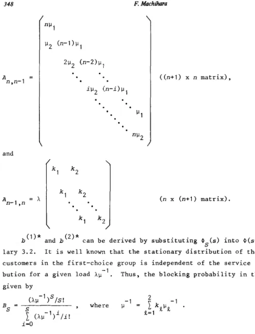
348 F. Machihara

«n+1) x n matrix),

and

(n x (n+1) matrix).

b(l)* and b(2)* can be derived by substituting

~s(s)

into

~(s)

in Corol-lary 3.2. It is well kno~l that the stationary distribution of the number of customers in the first-choice group is independent of the service time

distri-·-1

but ion for a given load A~ Thus, the blocking probability in this group is given by

where ~ -1

Hence, the input rate to the infinite trunk group, v, is given by

and thus

-1 v~

The variance v ~s provided by v

=

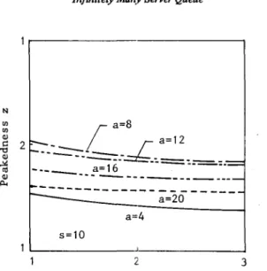
2b*(2) + a - a2

Figure 2 shows the effect of the coefficient of variation of service time, cs' on peakedness of overflow streams, z. We fit a hyperexponential distri-bution with balanced mean [13]. As Cs increases, z decreases monotonically.

N UJ a=8

~

2

::::~L:.::L-::

__ _

'i;l

-__

a=16

---=-=

Q) ...

-~

:.:.:.:.- - ;-20 --

----a=4 s=10 3 Coefficient of variation of service time Cs

Figure 2. Coefficient of Variation of Service Time VS Peakedness

(a = A)1-1)

4.

Concl usion

An MR/H la> queue having Markov renewal inputs and hyperexponential service m

times is analyzed. Stationary state distributions are derived at both the customer arrival epoch and an arbitrary time point. The most important meas-ures, the mean and the variance of the number of customers in the system at an arbitrary time are explicitly represented. By applying these results to the equivalent random method, it is possible to engineer telephone networks under the assumption that the service time distribution is hyperexponential.

ReferE!nces

[1] P.J. Burke: The Overflow Distribution for Constant Holding Time, Ben Syst_ Tech. J_, 50, PP. 3195-3210 (1971)

[2] E. ~inlar: Introduction to Stochastic Processes, Prentice-Hall Inc., Englewood Cliffs, New Jersey (1975)

f3]

V. P. Franken: Erlangsche Forme In fUr Semimarkowschen Eingang, Elect.ron. Informationsverarb. Kybernetik, 4" PP. 197-204 (1968)

350 F. Machihllra

and Customer-Dependent Exponential Service Times, Oper. Res., 20, PP. 907-913 (1972)

[6] L. Takacs: Introduction to the Theory of Queues, Oxford Univ. Press, New York (1962)

[7] R.I. Wilkinson: Theories for Toll Traffic Engineering in U.S.A., Bell Syst. Tech. J., 35, PP. 421-514 (1956)

[8] V.B. Iversen: Analyses of Real Teletraffic Processes Based on Computer-ized Measurement, Ericsson Tech., 29, PP. 3-64 (1973)

[9] E. Takemori, Y. Usui and J. Matsuda: Field Data Analysis for Traffic Engineering, proc. 11th Intl. Teletraffic Cong., Session 3.2B, 5, Kyoto, Japan (1985)

[10] F. Machihara, Y. Takahashi and Y. Usui: Individual Overflow Processes from the M

1, M2/M1, M2/S/S Loss System. Review of Elec. Corn. Lab., 34, PP. 561-567 (1986)

[11] L. Kosten: Ober Sperungswahrscheinlichkeiten bei Staffelschaltungen, Elek. Nachr. Tech., 13, PP. 5-12 (1937)

[12] G. Bretschneider: Die Berechnung von Leitungsgruppen fUr Oberfliessenden Verkehr in Fernsprechwahlanlagen, Nachrichtentechnische Zeitschrift, 9, PP. 533-540 (1956)

[13] P.M. Morse: Queues, Inventories and Maintenance, John Wiley, New York (1958)

Fumiaki MACHIHARA: Department of NTT Telecommunications Laboratories, 3-9-11 Midoricho, Musashino-shi, Tokyo 180, Japan