ASYMPTOTIC PROPERTIES OF STATIONARY DISTRIBUTIONS IN TWO-STAGE TANDEM QUEUEING SYSTEMS

Vol. 41, No. 1, March 1998

ASYMPTOTIC PROPERTIES O F STATIONARY DISTRIBUTIONS IN TWO-STAGE TANDEM QUEUEING SYSTEMS

Kou Fujimoto Yukio Takahashi Naoki Makimoto

Tokyo Institute of Technology

(Received May 1, 1997; Revised October 3, 1997)

Abstract This paper is concerned with geometric decay properties of the joint queue length distribution

A n 1 , n 2 ) in two-stage tandem queueing system P H / P H / q

-+

- / P H / c 2 . We prove that, under some

conditions, p h n 2 ) C(n2)r]n1 as n l -+ ca and p ( n l , n 2 ) C ( n i ) F 2 as n2 -+ ca. We also obtain the asymptotic form of state probabilities when nl is large or when n2 is large. These results prove a part of the conjecture of a previous paper [l]. The proof is a, direct application of a theorem in [7] which proves geometric decay property of the stationary distribution in a quasi-birth-and-death process with a countable number of phases in each level.

Introduction

Tandem queueing systems are basic models in the theory of queues and have been studied for a long time. However, because of complexities of their stochastic structure, their properties are scarcely known except for cases with product form solutions. They are simplest models of queueing networks as well as direct extensions of single queueing systems. Hence the study of them are expected t o connect the theory of single queueing systems with t h a t of queueing networks. In this paper, we prove geometric decay of the stationary state probability in a two-stage multi-server tandem queueing system P H / P H / c l -+ / P H / c 2 with a buffer of infinite capacity and with heterogeneous servers.

In the ordinary one-stage queue P H / P H / c with traffic intensity p

<

1, it is known t h a t the stationary distribution has a geometric tail [ 6 ] . Let ~ ( n ; zo, z1) be the stationary probability t h a t there exist n customers in the system while the phases of the arrival and service processes are iy and

z\

respectively, then

where (7, Co(zo), Cl(zi) and T ] are some constants and indicates t h a t the ratio of both sides

tends t o 1. These constants other than G can be easily obtained from the phase type rep- resentations of the interarrival and service time distributions. This kind of geometric decay property is very useful, for example, on the computation of the stationary state probabili- ties, or on the discussion of tail probabilities for estimating very small loss probabilities (e.g. less than 1 0 ' ) of the corresponding finite queue. The above result was further extended for the G I / P H / c queue with heterogeneous service distributions [5].

Our main concern here is t o prove a similar geometric tail property in the two-stage tandem queueing system P H / P H / c l -+ / P H / c 2 with heterogeneous servers.

In a previous paper [I], the authors have made a conjecture on the geometric decay of the stationary state probability in a single-server two-stage tandem queueing system PH/PH/1

-+

/PH/1 through a n extensive numerical experiment. Let n(n1, n2; IQ, 21, 12) be

Asymptotic Properties in Tandem Queues 119 the stationary probability that there exist n l customers in the fist stage and n2 customers in the second stage while the phases of the arrival process and the two service processes are iy, il and i2, respectively. Then the conjecture asserts that the stationary state probability decays geometrically as nl and/or n2 become large but decay rates and multiplicative constants may be different according to the ratio of nl and n2:

for large n-\_ and/or n2 such that n2

<

a n l ,

7r(n1,n2;^0^1^2) - -

G

c 0 (io)

Ci

(h)

Ci

(G)

~FT;',

I

for large n l and/or n2 such that n l

<

a 1 n2,

where a = - h ( q l / n l ) / 1 n ( q 2 / ~ ) and constants qk,

Tk

( k = 1,2) and C k ( i k ) , w k ) (k =

0 , 1 , 2 ) are determined from the phase-type representations of the interarrival and service time distributions.

In this paper, under a certain condition, we prove the geometric decay property (1.2) for the multi-server case P H / P H / c l -+ / P H / c 2 in two special cases, the case where n l

-+

oo

with n2 being fixed and the case where n2

-+

oo with n l being fixed. The proof uses a result on the Matrix-geometric form solution of a quasi-birth-and-death (QBD) process with a

countable number of phases in each level [7].

The remainder of the paper is constructed as follows. In Section 2, we describe our two-stage tandem queueing model and state our main theorems in Section 3. The result of

[7] is briefly summarized in Section 4, and we prove the main theorems for a single-server case PH/PH/l -+

/PHI1

in Sections 5 and 6. In Section 7 we give an outline of the proof for the multi-server case P H / P H / c l

-+

/PH/c2. In many places of the proofs, we use properties of solutions of four key systems of equations given in Section 3. These properties are proved in Appendix.

2 . Model Description

We denote by PH(a,

<&)

a phase-type distribution represented by a continuous-time, finite- state, absorbing Markov chain with initial probability vector

_-

_-

ii

= ( a , 0) and transition rate

-

matrix <& =

1

f

1

(see [4]). The phase-type distribution is said to be irreducible if "ya

+

@ is irreducible, or equivalently - a < &

>

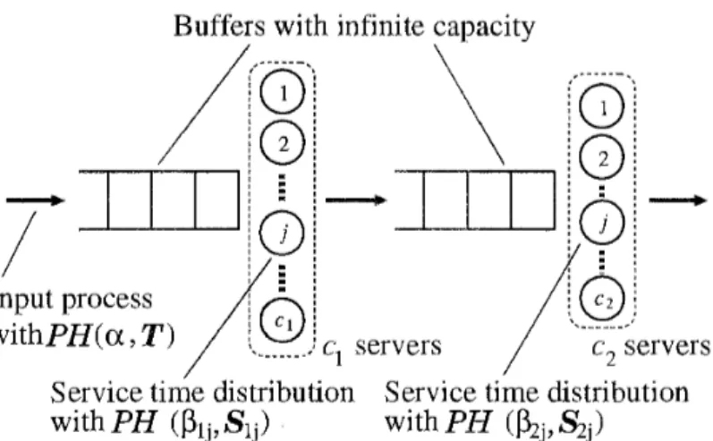
0.

We consider a two-stage tandem queueing system (Figure 1). Customers arrive a t the first stage to be served there, move t o the second t o be served there again, and then go out of the system. The k-th stage (k = 1 , 2 ) has ck servers and a buffer of infinite capacity, so that neither loss nor blocking occurs. Interarrival times of customers are independent and identically distributed (i.i.d.) random variables subjecting t o an irreducible phase-type distribution P H ( a , T). Service times a t the j - t h server of the k-th stage ( j = 1 , 2 , . . .

,

ck) are also i.i.d. variables subjecting t o an irreducible phase-type distribution PH(ftkj, S k j ) . These interarrival and service times are assumed to be mutually independent. Customers are served under the first-come-first-served (FCFS) discipline and those who find multiple servers being idle choose a n idle server randomly according to state-dependent probabilities. The state of the system is represented by a vector ( n l , "2; io; ill,

-

.

.

,

ilcl; i21,

-

.

- ,

i2Ca);

where nk is the number of customers in the k-th stage, in is t h e phase of the arrival process, and

k j

is the phase of the service process a t the j-th server of the k-th stage ( j = 1 , 2 , . . .

,

ck; k = 1,2). The index iy is interpreted to be equal t o zero if the correspond-

Buffers with infinite capacity

\

c, servers

/

c,, servers Service time distribution Service time distribution with

PH

(plj,

Sij)

with

PH

(h,

S;,)

Figure 1: Two-stage tandem queueing system

ing server is idle. Then the system behaves a s a continuous-time Markov chain, which we de- note by { X ( t ) } . For brevity of notation, we sometimes abbreviate the vector representation

. .

n l , n2; $0; 2 1 1 ,

.

. .

,

zlci; z21, . . .

,

Gcz) as (nl, n2; zO, zl, z2), where z1 should be interpreted a s a

vector (zll, .

.

.

,

zlcl) and as a vector (izl,

.

.

,

i2c2).

We denote the traffic intensity a t the k-th stage by pk = A/ where I/A is the mean interarrival time and l/pikj is the mean service time a t the j-th server of the k-th stage, and assume pi, p2

<

1 so t h a t the chain is stable and has stationary state probabilities

. .

~ ( ~ 1 , n 2 ; ~ 0 ; ~ 1 1 ~ - . . ~ ~ 1 ~ ~ ; ~ ~ 1 , . . - , & ~ ~

3. Main Theorems

T h e (marginal) queue-length distribution of the first stage clearly has a geometric tail as proved in [6], since the behavior of the first stage is not affected by t h a t of t h e second stage. Our concern is the tail property of the joint queue-length distribution of the first and the second stages or the asymptotic behavior of the stationary state probabilities.

We prepare some notations. Hereafter, k represents the stage number and takes a value 1 or 2, and j represents the server number and runs from 1 t o c^. We denote by I the identity matrix and e the column vector of all entries equal to 1. The order of them ma,y be finite or infinite and is understood so that expressions are well defined. If we need t o emphasize t h e order of them, we attach a suffix "0" or a double suffix LLkj'7. For example,

T O is the identity matrix of the same order as T and e k j is the column vector of the same

order as Skj with all entries equal to 1. We set

T~ = -Teo and ykj = -Skj ekj.

Then the Laplace-Stieltjes Transforms of the interarrival and service time distributions are given by

Now we shall state our main results. We start from the case with n l

-+

oo.

Asymptotic Properties in T a n d e m Queues 121 As will be proved in Lemma 8.1 in Appendix, the system of equations (3.2) has two solutions, one of which is (h, so, ~ 1 1 , . . .

,

sic,)

= ( 1 , 0 , 0 , . . . ,0). We will denote the other solution as (h, so, s n , . . .

,

slcl) = (vl, 00,011,. . .

,

olc1). Then from the stability condition p1

<

1, we will see in the same lemma that 0

<

771

<

1, 00

>

0 and 01,

<

0.

Using 771 above we consider another system of equations for h, so, sl1, . . .

,

slc1, s z l , . . .

,

szc2

The system of equations (3.3) has again two solutions as proved in Lemma 8.2. One of them is (h, so, ~ 1 1 , .

.

.

,

s l c , ~ 2 1 , . . .

,

Szc2) = (l, 0 0 , 0 1 1 , . .

.

,

olc1, 0,. .

.

,

O), and we will denote

the other as (h, 50, ~ 1 1 ,

- - -

S i c l 7 3 2 1 ,

. .

,

s 2 c 2 ) = (772; WO, ^ l 1 7

- -

^lc17 ^217

- - -

7 ^2c2)- Clearly wo = 00. Associated with this solution, we introduce row vectors

Using 771, 772 and vectors above, the first theorem is stated as follows.

Theorem 3.1. If 77;

<

1, for fixed n , io, i1 = (ill,

.

. .

,

ilcl) and =

(h;,

. . .

,

h),

the stationary state probability decays geometrically with rate 771 as n l --+ m:

The multiplicative constant G1(n2; io, ii, i2) decays geometrically with rate 772 as n2

--+

00:

where Co(i) is the i-th element of W O , Ckj (2) is the z-th element of W k j , and G2 is a constant

independent of n2, io,

G

and i2.

Next we shall state our result for the case where n2

--+

m. We will use symbols with bars for quantities related to this case.

As will be proved in Lemma 8.3 in Appendix, the system of equations for h, s o , s a l , . . .

,

s Z c 2

has two solutions, one of which is (h, so, s z l , . . .

,

szc2) = ( 1 , 0 , 0 , .

. .

, 0 ) . We will denote the other solution as (h, so, 5 2 1 , . . .

,

s 2 c 2 ) = (q2,

zo,

0-21, . . .

,

a2c2). For the solution, from the same lemma, we see that 0

<

TJ^

<

1, 0-0

>

0 and a^j

<

0.

has also two solutions, one of which is (h, s o , ~ 1 1 , . . .

,

slcl, s 2 ~ , . . .

,

sZc2) = ( 1 , ~ ~ ~ 0 , . . . , 0 ,

- -

0 ,. . .

,

osc2). The other solution is denoted as (h, SO, s l l , . . .

,

sic,, s 2 1 , . .

.

,

sac,) =

(v1,

V o ,

- - -

wll, . .

.

,

wlc1, ~ 2 1 , . . .

,

wzc2). Clearly a'2, = Associated with this solution, we introduce row vectors

-

W O = a

(qIO

- T ) ' and my = (oikjIkj - Skj)-l. (3.9)

Using 771, 772,

ql

and vectors above, the second theorem is stated as follows.

Theorem 3.2. If ql

<

q2

and

nl

<

v,,

for fixed nl, io, il = ( i l l , . . .

,

ilcl) and 22 =

( z ~ ~ ,

. . .

,

i2c2), the stationary state probability decays geometrically with rate 77, as n-s,

-+

oo: -

r ( n 1 , ~ 2 ; ? 0 , ~ 1 ~ ~ 2 ) G2(n1; ZQ\ ~ 1 ~ ~ 2 ) s 2 . (3.10) The multiplicative constant G ( n l ; io, il

,

i2) decays geometrically with rate

Tl

as nl -+ m:

-

G2(n1; Èo,i1,22

G

co(io)

m4

c2(22)

if;1

(3.11)

with

- - -

Cl (21) =

Cii

(211)

Clc1

(iic,) and C2(k) = c 2 1 (i21) C 2 c 2 ( 2 2 ~ ~ ) ~

where G ( i ) is the i-th element of WO, Cki(i) is the i-th element of TVkj, and

G\

is a constant independent of n l , in, i\ and 22.

Remark 1. The decay rates m. and Q have the following properties. These properties are easily proved from lemmas in Appendix.

The decay rate 771 is a monotone increasing function of pi, and

v1

4

0 a s pi

4

0 while 771 f 1 as p1 1. T h e other decay rate 772 is less than 1 if p2 is small but it may exceed 1 if p2 becomes large. 772 can be regarded as a function of both pl and p2. For fixed pi, it is a monotone increasing function of p2 and q2 $. 0 as p2 ^, 0.

A numerical experiment shows t h a t 772

<

1 in most of two-stage tandem queueing systems, and hence Theorem 3.1 holds in a wide range.

The decay rate

77,

is a monotone increasing function of p2, and Q ^, 0 as p2 $. 0 while

-

f 1 as p2 f 1. The other decay rate

v1

is a function of p1 and p2, and for fixed py, it is a monotone increasing function of pi. As pl .j, 0,

TJl

$. 0, and as pl f 1,

-?-

q2. This means t h a t

q1

may exceed 1.

For the condition 71

<

q2

t o hold, p2 must be greater than some positive value. Hence Theorem 3.2 holds only in some limited cases.

Remark 2. The authors have never succeeded t o give an intuitive interpretation for the condition 772

<

1 of Theorem 3.1 and the condition q1

<

v2

and

q1

<

772 of Theorem 3.2. Related discussions are given for single-server tandem queues M A P / P H / l

--+

/ P H / 1 in [3] and G I / M / l -+

/M/l

in [Z].

Remark 3. It is well known t h a t the marginal queue-length distribution of the first stage

Asymptotic Properties i n Tandem Queues

Theorem 3.2 hold, the marginal queue-length distribution of the second stage

has geometric tail, too, but with decay rate

v2.

Its proof requires some extra pages, and it will be presented elsewhere.

Remark 4. The constant Gl(n2;

h,

&) in Theorem 3.1 is given by the corresponding

element of p in Lemma 5.2 up to a multiplicative constant. Using the geometric decay property of pl(nl) in Remark 3, we can see that p up to a multiplicative constant gives the conditional state probabilities when nl is sufficiently large. From the proof of the lemma, p is directly derived from stationary distribution pn of a certain QBD process with a finite number of phases. Since pn is of the matrix-geometric form, we can easily obtain the value of Gl (n2; io^

i\^

i2) by numerical computation.

The constant G2(n1;

G,

il, i2) in Theorem 3.2 corresponds t o the element of

p

given in Lemma 6.2. I t is also easy to get numerical value of

p

from the steady-state distribution of a QBD process. When n2 is sufficiently large, using the geometric decay property of p2(n2) in Remark 3, the conditional state probabilities is given by

p

up to multiplicative constant. 4. Geometric Decay Property in a Quasi-Birth-and-Death Process with a Count-

able Number of Phases

To prove the theorems, we use the corollaries in [7]. These corollaries are summarized as Proposition 1 below.

Consider a continuous time positive recurrent Markov chain {X(t)} on the state space S = { ( m , ~ ) ; m , i = 0 , 1 , 2 , . .

.}.

The state space S is partitioned into subsets ,Cm =

{(m,

i } ;

i = 0 , 1 , 2 , . .

.},

m = 0,1,2, .

. .,

called levels. When partitioned by levels, the tran- sition rate matrix Q of {X(t)} is assumed t o have a block-tridiagonal form:

Such a chain is called a quasi-birth-and-death (QBD) process with a countable number of phases in each level. The stationary vector TT of the QBD process is also partitioned as (xO, TT!,

-

) according t o G ' s .

Proposition 1. We assume that diagonal elements of -B and -Bo are bounded by d(< W) from above and that there exist a positive constant 77

<

1 and positive vectors p and q satisfying

p (^-'A

+

B

+

= 0, (4.2)

n l p A q # n p c q , p e < m , and p q < m .

If TT' q

<

oo and if the matrix Q' formed from Q by deleting rows and columns corresponding

t o states in C,o is irreducible, then TT has a geometric tail:

For the proofs of Theorems 3.1 and 3.2 in the preceding section, we apply this proposition for partitions by the number of customers in the first or the second stage.

We also prepare some properties related t o phase-type distributions. We will denote by and @ the Kronecker product and the Kronecker sum operations.

Let P H ( a , a ) be a n irreducible phase-type distribution and put 7 = - @ e . Then the LST of the distribution and its derivative are given by

' S ' * ( s ) = a ( s I - @ ) ' l 7 and < ^ * ' ( s ) = - a ( ~ I - @ ) - ~ ~ . (4-7) Especially, the mean of the distribution is given by -@*'(0) = a(-@)-2-)' = a ( - @ ) ' e . Note that @*(S) can be considered as a function of S on the interval

(4,

oo) where

<

0 is the abscissa of convergence.

Lemma 4.1. For h

>

0 and s

> 4,

the equation

has a positive solution X if and only if ^?*(S) = h. If <^*(S) = h, then X = a (S I - @ ) l is a unique positive solution of (4.8) up t o a multiplicative constant.

Proof. From (4.8) we have X ( s l - @) = ( h 1 x 7 ) a and hence

Postmultiplying 7, we have x-y = h l x - y ? * * ( s ) . This implies t h a t , if the equation (4.8) has a positive solution, then <^*(S) = h. Conversely, if @*(S) = h , by substituting X with

a (S I - @ ) l the left hand side of (4.8) is rewritten as

Hence X = a (S I - @ ) l is a solution of (4.8). The positivity of a (S I - a ) ' is clear from

the irreducibility of the distribution. The equation (4.9) indicates that a (S I - @ ) l is a

unique solution up t o a multiplicative constant. 1

Lemma 4.2. For irreducible phase-type distributions PH(afli} with 7, =

-Re,

z = 1 , 2 , . . .

,

c, and for positive numbers hi, h 2 , . . . , h o the vector equation

has a positive solution X if and only if there exit real numbers S', 5 2 , . . -

,

sc such t h a t @,*(S,) = hi, i = 1 , 2 , . . . , c , and s l + s 2 + - - - + s c = 0. The solution is given by X = x l @ - - - @ q with X, = a, (S, I, - @ , ) l , i = 1 , 2 , . . .

,

c, u p t o a multiplicative constant.

Asymptotic Properties in h d e m Queues

Proof. First we prove "if" part. From Lemma 4.1 we have

Thus X is a solution of (4.10). For the proof of "only i f part, we write f = ( h p 71 a1

+

+ l ) @ @ ( h 1 7 ac

+

$c). From the irreducibility of P H (ai, + i ) , the matrix f is irreducible

and its Perron-Frobenius eigenvalue is simple. The equation (4.10) implies the Perron- Frobenius eigenvalue is equal to zero.

Since f is a Kronecker sum of c smaller matrices, its simple Perron-Frobenius eigenvalue is a sum of Perron-Frobenius eigenvalues of the smaller matrices. From Lemma 4.1 such eigenvalues have t o satisfy (S,) = hi and sl

+

3 2

+

- -

+

sc = 0. Â

5 . Proof of Theorem 3.1 for Single Server Case

First we prove Theorem 3.1 for the single server system PH/PH/l

-+

/ P H / l . In this case, cl = c2 = 1 and the state of the Markov chain { X ( t ) } is written as ( n l , 722; io, il, i2) in which il and i2 are no longer vectors but integers. Double suffices in symbols such as S k j and w k j

are also replaced with a single suffix as S k and wk.

We arrange the states (nl, n2; 12) in lexicographic order and partition the state space according to 7x1, i.e., we let

L m = { ( n l , n 2 ; i o , i l , i 2 ) ~ n l = m } , m = O , 1 , 2

,....

(5-1) We denote by Q the transition rate matrix of the chain corresponding to the arrangement above and by TT = (x0, T T ~ ,

. . - )

the stationary vector partitioned according to G ' s . Then

Q is of the block-tridiagonal form as (4.1) with 7 0 " @ Jl 7 0 0 : @ J l @ 1 2 A = 7 o a @ I1@ 1 2

B

and

c

Then { X ( t ) } is regarded as a QBD process with a countable number of phases in each level. Now we shall apply Proposition 1 and prove Theorem 3.1 by taking V =

v1

and suitably defining vectors p and q. First we introduce several matrices and vectors including q , and then we check in Lemmas 5.1 5.3 t h a t the condition (4.2) (4.5) of t h e proposition hold. T h e geometric decay of the limiting vector p will be proved in Lemma 5.4.

Let

Then from (5.2), (5.3) and (5.4)

We define row vectors and column vectors as

U,, = a ( o o I o - T ) - l , _{U1 = /31(0111} - S1)-l, U 2 = /32(-S2)-l,

v, = (ooIo - T)-'-y0 and v1 = (01Jl - S l ) - l 7 , . (5.6)

Since w o = oo, the vector u0 is the same as W O defined earlier. But for symmetry of

expressions, we introduce another symbol here. Note t h a t , from Lemma 4.1, uo is a solution of the equation uo('n~170a

+

T) = oouo. Other vectors are solutions of similar equations, too. These equations will be frequently used in the proofs of subsequent lemmas.

From (4.7) and the fact that (vl, 0 0 , o l ) is a solution of the equation (3.2), these vectors are related with LST of interarrival and service time distributions as follows.

Since A

+

B

+ C

=

(ipc170a

+

T) CD (i)171/31

+

s l ) CD

(72/32

+

s 2 ) , it follows from Lemma 4.2 t h a t

Let us define a column vector

Asymptotic Properties in Tandem Queues 127

Proof. The positivity of q is clear from the definition. The vector K q is written as

-&(vo

8

v1 R

e;)

+

Bo(vo

8

v l )

( A

+

B)(vo

8 v1 e z )

+

C1(vo

R V ' )

( A +

B + G ) ( V O @ v 1 8 e;)

( A

+

B

+

C){vo R v1

8

ez)

From (5.8) the subvectors of K q corresponding t o ,Cm, (m

2

2), are equal to zero vectors. For the first two subvectors we can also check that they are equal t o zero vectors. I

To prove the next lemma, we need another notation. For an arbitrary column vector

4

we let d i a g ( 4 ) be the diagonal matrix having elements of

4

in its diagonals. The operator

d i a g ( - ) satisfies the following relations for column vectors

4

and i f s :

Lemma 5.2. If 77;

<

1, there exists a positive vector p such t h a t

pK = 0 , pe

<

oo, and pq

<

oo.

Proof. To use a property of an ergodic Markov chain, we transform K so that it becomes

a transition rate matrix. Let D = d i a g ( q ) and

where

Do

= d i a g ( v o 8 v l ) and

D

= d i a g ( v o 8 vl 8 e^j. Since K D e = D ^ K ~ = 0 , K D

is a transition rate matrix of a QBD process with a finite number of phases in each level. Theorem 3.1.1 in [4] says that K D is ergodic if and only if

where TT is a positive row vector such that

From (5.8) we know t h a t TT is written as (uo 0 u1 @I Â ¥ u s D up t o a multiplicative constant.

and

Therefore, the difference of the both sides of the inequality (5.10) is given by

If

7 7 ~

<

1, the quantity in the braces is positive from Lemma 8.5 in Appendix, and hence the inequality (5.10) holds. This proves t h a t K D is ergodic under the assumption of Theo- rem 3.1.

Since K D is ergodic, there exists a positive vector pn such that p D K D = 0 and pDe = 1. Then,

p = P D ~ - l (5.12)

is the desired positive vector. In fact,

and

p e < d 1 p q < dl

<

00,

where dl is a positive number such that e

<

dl q .

Lemma 5.3. For p given in (5.12) we have 77,1pA

>

p C q .

Proof. Let

then

Note that a postmultiplication of E implies a n aggregation of states into aggregated states with common states of the arrival process and the service process a t the first stage while the state of the second stage is ignored. Postmultiplying E to the equality p K = 0 and applying (5.13), we have

From Lemma 4.2, p E is a constant multiple of uo u l . If we let the multiplicative constant be H, we have

Asymptotic Properties in Tandem Queues 129 The quantity in the braces of the right most hand side is positive from Lemma 8.6 in

Appendix, and the inequality of the lemma holds. I

Lemmas 5 . 1 ~ 5 . 3 above show that the constant q1 and positive vectors p and q satisfy the conditions ( 4 . 2 ) ~ ( 4 . 5 ) in Proposition 1. The remaining is to show that 71-19

<

oo and

that the matrix Q' is irreducible. The former is trivial from the fact that there exists a positive number d2 such that q

<

d2e. The latter is easily checked using the irreducibility of the interarrival and service time distributions. Thus we have proved (3.5) of Theorem 3.1.

To prove the tail property of p, we introduce a subpartition of each

C,rm

m

>

1,

and we divide the vector p as (p(O), p ( l ) , . .

. ) according to this subpartition.

Lemma 5.4. The vector p given in (5.12) has a geometric tail:

where G' is a constant and W O , W!

(=

wl1) and w 2 (= wzl) are vectors defined in (3.4).

Proof. By the QBD structure of the transition rate matrix KD, we can apply the matrix analytic theory by Neuts

[4].

Let

h

be the rate matrix of K D . Then it is the minimal non-negative solution to the matrix equation

Since p = pD D ' , we know that

-

nt

-

-1

p(n2) = ~ ( l )

D

R~ D as n2 Ñ oo,

where G" is a constant,

fi

is the Perron-Frobenius eigenvalue of and

in

is a corresponding left eigenvector: X D

RD

=

fi

b.

Then by premultiplying XD to the equality (5.15), we have

Since fj

<

1, from Lemma 4.2 and Lemma 8.1, & Dis a constant multiple of w o @w1 SW,:

This proves the lemma.

% D - = G'" w o 0 w l Si w 2 .

I Lemma 5.4 proves (3.6) of Theorem 3.1, and this completes the proof of the theorem.

6 . Proof of Theorem 3.2 for Single Server Case

Next we prove Theorem 3.2 for the single server system P H / P H / l

-+

/PH/1.

In this section we use the same convention for the double suffices as in the last section.

We rearrange the states (nl, n2; io, il, i2) of {X(t)} first in the order of n2 and then in

the lexicographic order. We define a new partition of the state space by

-

~ ~ = { ( n ~ , n ~ ; i ~ , i ~ , i ' ~ ) ~ n ~ = r n } , r n = 0 , 1 , 2

, . - . .

( 6 - 1 ) We denote by Q the transition rate matrix of the chain corresponding to the arrangement above. Then, if we partition according to

G'S,

Q

is of a block-tridiagonal form

where

and

We denote by TV =

(

TO, TVl,

- -

)

the stationary vector of {X(t)

} partitioned according to

-

Lm7s.

We shall show that the conditions of Proposition 1 hold if we take =

%

and if we define vectors

p

and ?j suitably. Similar to the preceding section, we first introduce several matrices and vectors including

q,

and then we check in Lemmas 6.1 6.3 that the condition (4.2)

-

(4.5) of the proposition hold. The geometric decay of the limiting vector

p

will be proved in Lemma 6.5.

Asymptotic Properties in Tandem Queues

Let

Then from (6.3), (6.4) and (6.5)

n A A0 = y o a @ / 3 l 0 1 2 7 A =I

0

_{1 1}

0

_{1 2 ,} A BO = T M 2

+

~ Z I O @ 7 2 / 3 2 ,

B

= T @ S l ~ S z + i ? ~ J o @ I i @ 7 2 1 8 2 1 A n Cl =

q 2 I o

g T~ I 2 and C = iiYIJo @ 7 1 / 3 1 @ 1 2 -

We define row vectors and column vectors as

- -

uo = a ( f i I o - T ) - l ,

m

= ,Bl (-Si)-l, ~2 = ^ ( % I 2 - S2)-',

-

v. = (voIo - T ) ' ~ ~ and 5 2 = (F212 - S - s ) ' - f , .

Since =

v2,

the vector

u2

coincides with W 2 defined in (3.9). These vectors are solutions of equations of a type given in Lemma 4.1. They are related with LST of interarrival and service time distributions as follows:

-

U,-,To =

avo

= T * ( T o ) =

q2,

B 1 f l = ,B1w1 = S ^ i ) =

qal,

- - -

U ~ V ~ = - T * ' ( ~ ' ~ ) , u ~ < ' ~ = - s ~ ' ( ~ ' ~ ) and t t 2 e = - s i t ( 0 ) . (6.9)

We define

-

Q =

Lemma 6.1. The vector

o

is positive and satisfies

Kg

= 0 .

The proof is straightforward from Lemma 4.2.

Lemma 6.2. If

ql

<

q2,

then there exists a positive vector

p

such that

p z = 0 ,

p e < o o and m < o o .

1--

A

where

DO

= diag(vn 8

6)

and D = d i a g ( 6 8 el 8

&).

G

is a transition rate matrix of a QBD process with finitely many phases in each level. The ergodicity of is proved as follows.

From Lemma 4.2, the vector 'K =

(ao

@ 8

u2)

5

satisfies the equation

A direct calculation shows that

--l--

= S*) {T* (F,,) S?' (0) - T*' (o'o)

S:

(Q)}

If

v1

<

q2,

the quantity in the braces of the right most hand side of the above equation is positive from Lemma 8.7 in Appendix, and hence from Theorem 3.1 .l in [4] the Markov chain

G

is ergodic under the assumption of Theorem 3.2.

Thus there exists a positive vector 6 such that p f l E = Q and %e = 1. Then,

-- 1

p

=

pDD

(6.11)

is the desired positive vector. In fact

- - - -1

p K = p - r , K r j D = O , p g = p ~ , e = l < m and

p e < d l p g < d l

<oo,

where is a positive number such that e

<

dig. Â

Lemma 6.3. For

p

given in (6.11) we have

_>

n2

pm.

Proof. We note that, from (6.6) and (6.7),

K

is written in the form of a Kronecker sum

K

=

E<Â

( S 2

+

5)272/32 -

M ) .

(6.12)

with some matrix

E.

In order to derive a detailed structure of

p,

we shall decompose related matrices and vectors in a similar manner t o (6.12).

K-r,

is decomposed as

where

Asymptotic Properties in Tandem Queues 133 The matrix

L

in (6.12) is given as in (6.14) by removing hats. Zj and

D

are decomposed as

q =

qr

8

v2

and

D

=

R

0 diag(&), where

and DT = d i a g ( e ) .

It is easily checked that ?jr

>

0 and

G-,

= 0 , or equivalently

LDe

= 0. Hence

G

is a transition rate matrix of a QBD process with a finite number of phases in each level. The ergodicity of is clear from that of

S,

and there exists a stationary probability vector

p-rrj

of the chain: _-

pLDLD==O

and p-LDe=l.

Using this

b,

we c a n decompose

p

and as follows:

Now we evaluate the both sides of the inequality of the lemma. Since

C q

=

7/y1

qz@h

we have _-

-_l - -

% p C q

= ( a 2 f 2 ) '

pm-

<lT

È2T =

R

( u ~ v ~ ) ~ , (6.15) where we use the relation

qz

= w e = l . On the other hand, since

we have

Note that eo (â‚ y1 = ( I o @ 7

/3

)(co (â‚ e l ) . This means that the i t h element of eo 0 71 is 1 1-

the rate that the Markov chain LE a t state ( n ,

i )

goes down to level ( n - 1 ) . Hence the

quantity (6.16) is the rate that the chain

LE

goes one level down in the steady state. From the balance equation, this rate is equal to the rate that the chain goes one level up:

This indicates that EZ can be regarded as the stationary probability vector of a Markov chain with transition rate matrix T

+

T 2 J 2

+

q21q00^ and is given by

-

p m

-E,

= ( T Z ~ ' ~ ' ~ ) '

a.

d i a g ( 6 ) . Thus, from (6.17), we have

--l --

q2 p A

q

= ( U ~ V ~ ) - ~ U. diag(v0) f o =

( $ Q )

S ri,.

Therefore, from (6.15) and (6.18) we have

From Lemma 8.8 the right hand side is positive, and this proves the lemma. I

Lemma 6.4. If q1

< q 2 ,

t h e n w

<

m . Proof. Since 71-1

<

we have

The behavior of the first stage of our tandem queueing system is not affected by the second one, and the stationary marginal probability vector ~ ~ of the first stage decays ge- z o ~ ometrically with rate ql as nl Ñ? m [6]. Since

q

decays with rate the inner product

Tmij is finite if q1

/v2

<

1. I

To see the asymptotic form of

p,

we consider a subpartition of each

L,

-

I n = { ( n l ; z 0 , i l , i 2 ) ~ = n}, n = 0 , 1 , 2

, . . . ,

and denote by

p

=

(p(O), p(l),

-

- )

the row vector

p

partitioned according to in's. Lemma 6.5. If

vl

<

1, then

where

G'

is a constant and

m,

(=

wl1)

and

m2

(=

?21) are vectors defined in (3.9) Proof. In a similar manner to the proof of Lemma 5.4, we apply the matrix analytic theory by Neuts [4] t o the rate matrix

G.

Let

%

be the rate matrix of

G

satisfying

Since

p

= we know that

~ n---l l

--

W

cl1

f ~+ D ^ l

Asymptotic Properties in T a n d e m Queues 135 A

where

G"

is a constant,

77

is the Perron-Frobenius eigenvalue of RE and

Sn

is the corre-

A

spending left eigenvector:

%

RD = Q+. Then by premultiplying t o the left hand side of (6.20), we have

--l

0 = % D

(fj-l,Z+B+fjC)

--l

From an extended version of Lemma 4.2, in order that the positive vector % D satisfies the above equation, there exit SO, sl and 5 2 such that

These equations are the same as (3.8) in the single server case, and hence s o = Uo, sl = U1, s2 =

a2

and

TJ

= since

TJ

has t o be less than 1. Again from Lemma 4.2, we know that

A - _{1 -///}

XED

= G

Wo<S)iZlCg)W2,

where

G / /

is a constant. This proves the lemma. I

Lemma 6.5 proves (3.10) of Theorem 3.2, and this completes the proof of the theorem.

7. Extension to Multi-server Case

The proofs in Sections 5 and 6 for Theorems 3.1 and 3.2 can be extended straightforwardly to the case with heterogeneous multiple servers in each stage. In this section, we give brief comments on the proofs of the theorems.

The state space of the Markov chain { X ( t ) } is divided in a similar manner t o (5.1), but here il should be regarded as a vector (ill,. . .

,

ilcl) and ia as a vector (ill,. . .

,

ilcl). In this case matrices A , B and C in (4.1) are of the form

B o o

B10 B11

Â¥clcl- B C l C l

BCl+lCl B C l C l

and

where

and other matrices are very complicated for writing down explicitly here since

Cm

for 0

<

m

<

c2 consists of states corresponding to various combinations of busy and idle servers. The proof of Theorem 3.1 for the multi-server case is parallel t o t h a t for the single server case given in Section 5. In this section, we use some symbols without explicit definitions if the meaning of them are easily understood from the corresponding ones defined for the single server case. For the solution

(vi,

0 0 , a n , . . .

,

olQ) of the equation (3.2), we define vectors

u0 = a ( o o I o - T)-',

and

vi,

= (%Ilj - S y ) 1 7 1 j

,

j = l , 2

,...,

cl.

These vectors satisfy similar relations t o (5.7). T h e vector q is defined as

where en is the column vector of the same order as the number of states in with all entries equal t 0-1.

Asymptotic Properties in T a n d e m Queues 137 For the existence of p, we extend Lemma 5.2 t o multi-server case. That is, if we put

then p exists iff

+ ? { D - ( ~ ~ ' C ~ ~ J @ ~

<

+ ? ( D ~ B ~ ~ ~ ~ ~ ) e . By definitions, this inequality is equivalent to the following one:

^

1

>g-

1 ill ,^l

sl'j

(01,) ,=l

S;;

(0)

If Q

<

1 the inequality (7.5) holds by Lemma 8.5 in Appendix, and hence Lemma 5.2 is extended t o mult i-server case.

A similar argument t o the above shows that Lemma 5.3 holds for multi-server case. In fact, if we let

then

For p, we postmultiply E to the equality pK = 0 to have

From Lemma 4.2, pE is a constant multiple of u 0 8 ull (8

- -

8 ulcl. Let H' be the

multiplicative constant, then we have

1 C l

1 C l C l

= H ~ - U ~ V ~

S

n

u l k v l ~ .= P - T * ~ I ~ ~ )

rn-s~tm-

E

{yL(olk)

Hence the inequality of Lemma 5.3 is equivalent t o 1

til

<

-T* (00) til

This holds from Lemma 8.6, and hence Theorem 3.1 is proved for the multi-server case. We can derive a proof of Theorem 3.2 for the multi-server case in a similar manner. We omit the proof here.

8. Appendix

In this section, we prove various properties of the solutions of the four key systems of equations (3.2), (3.3), (3.7) and (3.8) given in Section 3.

Lemma 8.1. _{The system of equations (3.2) has two solutions, one of which is (1,0,0,} . . . , 0 ) . For the other solution

(vl,

00, oil,. . .

,

olci),

vl

<

1, 00

>

0 and olj

<

0.

Proof. From the second equation of (3.2), we have

Since S$(sG) is a monotone decreasing function, the relation (8.1) defines slj as a function of 511. Then, from the third equation of (3.2), so = -sl1 - 3 1 2 - - sic, is also interpreted

as a function of sl1. Since so is a monotone decreasing function of sll, we may take so as an independent variable and regard sll, 5 1 2 , . . .

,

sic, as monotone functions of so. For brevity of notations, we introduce a function

Then the system of equations (3.2) can be rewritten as

Now we show t h a t the function U; (-so) is a logarithmic-convex function, t h a t is, log U: (-so) is a convex function and satisfies

T h e first differentiation U:'(-S~) can be obtained as follows. Differentiating both sides of the second equation of (8.3) by S O , we have

Asymptotic Properties in Tandem Queues

Substituting (8.5), we have

and hence

For ?7~"(-so), differentiating both sides of (8.6) by so we have

And hence

Therefore,

Since

S;

(slj) is a logarithmic-convex function of slj, the term between brackets is positive.

Therefore, U: (-so) is a logarithmic-convex function of SQ.

We denote by (r, m ) the domain of T*(so) and by (Qlj, m) the domain of

S 3

(slj). Then f (so) = T* (so)UT (-so) is defined on ( r , -

zl

Olj). It is trivial that so = 0 is a solution

of the equation f (so) = 1. This solution leads us to a solution (h, SO, ~ 1 1 , ~ 1 2 ,

. . .

,

sic,) =

( 1 , 0 , 0 , 0 , . . . , 0 ) of (3.2). Since f (so) is a logarithmic-convex function with limSoir f (so) =

limsoT- elj f (so) = oo, the equation f (so) = 1 has another solution so = 00. We note that, if p1

<

1 then

Since UT1(0) is negative, we have fl(0) = ~ " ( 0 ) - u;'(o)

<

0. Thus we know that 0 0

>

0. From the monotonicity of 5';- (slj), this solution leads us to another solution of (3.2)

where 71

<

1 and

<

0. Â

Lemma 8.2. The system of equations (3.3) has two solutions, one of which is (1,o-o,o11,

-

S, o-lc1,0,

-

- , 0 ) .

Lemma 8.3. The system of equations (3.7) has two solutions, one of which is ( 1 , 0 , 0 , . . . ,0).

-

For the other solution

(q2,

To, o"21,. . .

,

aic2),

ii2

<

l, 3 0

>

0 and

as,

<

0.

Lemma 8.4. The system of equations (3.8) has two solutions, one of which is

-

(1, 0-0, 0, . . .

,

0, Tz1, - . .

,

0-2c2).

The following four lemmas are used in Sections 5 and 6. Since all of them can be proved in a similar way, here we give a proof of Lemma 8.5 only.

Lemma 8.5. If q2

<

1, then

Proof. Similar t o the proof of Lemma 8.1, we introduce two functions

and consider the equation

Since f2(U;) is logarithmic-convex, this equation has two roots, 0 and a2. If q2

<

1, then 02

<

0 from (8.9) and fn(0)

>

0. This implies t h a t

and hence

From a similar equation to (8.6), we prove (8.8).

Lemma 8.6.

Lemma 8.7.

Asymptotic Properties in T a n d e m Queues ₁₄₁

Acknowledgments

T h e authors are grateful t o anonymous referees for their valuable comments which improve the exposition of the paper.

References

[l] Kou Fujimoto and Yukio Takahashi. Tail behavior of t h e steady-state distribution in two- stage tandem queues: Numerical experiment and conjecture. Journal of the Operations Research Society of Japan, 39(4): pp.525-540, 1996.

[2] A. Ganesh and V. Anantharam. Stationary tail probabilities in exponential server tan- dem queues with renewal arrivals. In Frank P. Kelly and Ruth J . Williams, editors, Stochastic Networks: The IMA Volumes in Mathematics and I t s Applications volume 71, pages pp.367-385. Springer-Verlag, 1995.

[3] Naoki Makimoto, Yukio Takahashi, and Kou Fujimoto. Upper bounds for the geometric decay rate of the stationary distribution in two-stage tandem queues. Research Report on Mathematical and Computing Sciences B-326, Tokyo Institute of Technology, 1997. [4] Marcel F. Neuts. Matrix-Geometric Solutions in Stochastic Models. The John Hopkins

University Press, 1981.

[5] Marcel F. Neuts and Yukio Takahashi. Asymptotic behavior of the stationary distri- butions in the GI/PH/c queue with heterogeneous servers. Zeitschrift fur Wahrschezn- lichkeitstheorie und verwandte Gebiete, 57: pp.441-452, 1981.

[6] Yukio Takahashi. Asymptotic exponentiality of the tail of the waiting time distribution in a PH/PH/c queue. Advances in Applied Probability, 13: pp.619-630, 1981.

[7] Yukio Takahashi, Naoki Makimoto, and Kou Fujimoto. Asymptotic properties in a quasi-birth-and-death process with a countable number of phases. Research Report on Mathematical and Computing Sciences B-321, Tokyo Institute of Technology, 1996.

Kou FUJIMOTO: fujimoto@is.titech.ac. jp

Yukio TAKAHASHI: yukioQis

.

t itech. ac

.

jp

Naoki MAKIMOTO: makimotoQis. titech. ac. jp

Department of Mathematical and Computing Sciences Tokyo Institute of Technology