NEWTON'S METHOD FOR ZERO POINTS OF A MATRIX FUNCTION AND ITS APPLICATIONS TO QUEUEING MODELS

(1)

Vol. 43, No. 3, September 2000

NEWTON'S METHOD FOR ZERO POINTS O F A MATRIX FUNCTION AND ITS APPLICATIONS T O QUEUEING MODELS

Shoichi Nishimura Atsushi Harashima Science University of Tokyo Mitsuba Co.

(Received May 13, 1999; Revised December 22, 1999)

Abstract Let R(z) be a matrix function. We propose modified Newton's method to calculate zero points of detR(2). By the modified method, we can obtain accurate zero points by simple iterations. We also extend this problem to a multivariable case. Applications to the spectral analysis of M/G/1 type Markov chains are discussed. Important characteristics of these chains, e.g., the boundary vector and the matrix G, can be derived from zero points of a matrix function and corresponding null vectors. Numerical results are shown.

1. Introduction

Let R ( z ) be a matrix function. In this paper, we consider Newton's method to obtain zero points of detR(z). At first, we propose a modification of the direct Newton's method and its extension it to a multivariable case. Second, applications of this work to the spectral analysis of M/G/1 type Markov chains are discussed. Important characteristics of these chains, e.g., the boundary vector and the matrix G, can be derived from zero points of detR(z) and corresponding null vectors of R ( z ) . Finally, numerical results are shown.

An M / G / l and a G/M/1 type Markov chains, introduced by Neuts [l11 are general- izations of an M / G / 1 and a G/M/1 queue. Because these models have many applications t o telecommunication techniques, they have received investigation in the last decade. The state space of these Markov chains is two-dimensional: the first element of state being level

n = 0,1, . . . which can be interpreted as the number of customers in the system) and the second element of the state; the phase ( i = 1, . .

.

,

M ) . By introducing a phase, we may rep- resent a state of a telecommunication system, i.e. a state of correlated inputs to the system or a state of service modes. The problem is to obtain the boundary vector of the stationary probability distributions from the transition probability matrix of a block Toeplitz form. The boundary vector is obtained by introducing the matrix G, the phase transition probability matrix for the first passage time from a level n

+

1 to a level n, and calculating the stationary probability vector of G (see Neuts [l11 and Lucantoni [g]). The matrix G is given by the minimal nonnegative solution of a nonlinear equation. When we calculate it numerically by an iteration method, at some point a truncation of level ( n = 0,1,

.

. .) is necessary.

The transform method for the boundary vector has been studied in series of papers by Gail et al. [ 5 ] , [6] and [7]. The vector generating function of the stationary probability is represented by the boundary vector and the matrix function. If the process is ergodic, then by using zero points of determinant of the matrix function on the unit disk and corresponding null vectors, the boundary vector is uniquely determined by the system of linearly independent equations.

(2)

Newton's Method for Zero Points of a Matrix Function 397

Recently in order to derive the boundary vector, several methods have been investigated. Algorithms for the calculation of the matrix G are obtained by using Newton's method in Latouche [8] and by using the cyclic reduction technique in Bini and Meini [2]. Under the assumption that R(z) is a matrix polynomial, spectral analysis is discussed in Mitrani [10]. To obtain null vectors of the matrix G, the invariant subspace approach is introduced by Akar and Sohraby [l] if the matrix function is rational. The fast Fourier transform is an approximate method with a wide use. Its application to an M / G / l type Markov chain is discussed (see Bini and Meini [2]). There is a trade-off between computation time and accuracy. If we want to obtain an accurate value of the boundary vector, we need a large amount of computational time and a large memory.

The motivation of this paper is how to calculate accurate zero points numerically. For this purpose, we propose the usage of Newton's method because we can easily obtain accurate values of zero points by simple iterations. Moreover, suppose that a roughly approximated value obtained by some method. We may set it as the initial value of Newton's method. In Theorem 1, we modify the direct Newton's method. The direct usage of Newton's method implies M

+

1 determinant calculations in each step of the iteration. By the modified method, however, it is executed by a sweeping-out method. The latter is accomplished by a smaller computational time than the former. In Theorem 2, the modified method is extended to a multivariable case. In Section 3, assuming that all eigenvalues are distinct, we get a simple proof that the boundary vector is uniquely determined by the system of equations in Proposition 3. And we also consider applications of Newton's method in a niultivariable case. It is proved in Theorem 4 that the spectral equation for a M A P / S M / l queue is divided into two equations of small size matrices. In Theorem 5, the similar result is obtained for a single server queue whose arrival process is a superposition of independent Markovian arrival processes. In Section 4, numerical calculations of eigenvalues of a M / G / l type queue are shown. The computational time and the speed of the convergence are shown. 2. Newton's Method

2.1. A single variable case

Suppose that R(z) = [ry(z)] (i, j = 1,.

. .

, M ) is an M X M matrix function of 2. Let us

consider the problem to solve the equation

det R ( z ) = 0 (1)

by using Newton's method.

Setting ZQ E

C

as an initial value and applying Newton's method to ( l ) , we get the

sequence {zk} such that

(3)

calculations of M

+

1 determinants of M X M matrices appear in Equation (2). To reduce

computational time of the direct Newton's method (2) to the problem ( l ) , we propose the following theorem.

Theorem 1 Suppose that a matrix X ( z k ) satisfies the linear matrix equation

Equation (2) is rewritten as

where t r X is the trace of a matrix X ,

Proof. Consider the M X M matrix X ( z ) = [xij(z)] (i,j = 1,.

. .

,

M ) which satisfies

The j t h column of X ( z ) satisfies

By Cramer's rule, xjj(z), the j t h diagonal entry of X ( z ) , is given by 1 xj3(z) = det R(z) Since t r X ( z ) becomes we get d - det R(z) = det R(z)

-

trX(z). dz

(4)

In the iterative formula (5), trX(zk) can be calculated by a simple sweeping-out method as follows. Suppose that the matrix R(zk) and

- ~ - R ( Z ) I ~ = ~ ~

are transformed to an upper triangular matrix [fi,(zk)] (i, j = l , .

. .

,

M) and [?!.(zk)] (i, j = 1,.

.

,

M ) by the same

zJ.

elementary transformation, respectively. That is, (5) is written as

Then xjj(zk) ( j = 1,

. . .

,

M), the j t h diagonal entry of X ( z k ) , is obtained from the formula

To compute [Fij(zk)] (i, j = 1,.

. .

,

M) and [?'.,{zk)] (i, j = l , . .

.

,

M ) requires :M3

+

0 ( M 2 ) multiplications in the elementary transformation. And M3

+

0 ( M 2 ) more multiplications are needed in the procedure to determine all diagonal entries of X(zk). So the total computational cost of each step by using ( 5 ) is 0 ( M 3 ) . The other way, in the iterative formula (2), calculations of M

+

1 determinants of M X M matrices are needed. Since the cost

of calculation for a determinant of an M X M matrix is $M3

+

0 ( M 2 )

,

the cost in each step is O(M4). Thus the iterative formula (5) has an advantage over the formula (2) in the computational time. Moreover, the iterative formula (5) is simpler than (2). So it is well-suited for creating programs of numerical computations.

2.2. A multivariable case

In this subsection we consider multivariable Newton's method solving zero points for determinants of matrix functions. For f = l ,

. . .

,

I<, let R6(z1,

. . .

,

zI<) = [rÃˆe(z1

.

,

zIc)] (i, j = 1,

.

,

Me) be Mf X Mf matrix functions of I{ variables 21, .

. .

,

ZK. We now consider

the problem to solve the system of K equations

det R l ( z l , . . .,Q) = 0 det -RIi-(;?!,.

. .

, z K ) = 0.

(0)

Setting (zl

,

. . .

, z P ) as a initial vector and applying Newton's method to the ~ r o b l e m (g), (k)

we get the vector sequence {(%

,

. . .

,

z y ) } such that

where

-L det R1 (zl,

. . .

,

zK)

-

. _-^-_{azv det R1 (zl}

,

_.

_{. .}

_,

_zIt-) J ( z 1 , .

. .

,

zIi-) =

(5)

where the symbol T means the transposition of a vector. We can rewrite (9) as

Theorem 2 For f , r , = 1 , . .

.

,

A', let ~ ( ( ~ ) ( z ( ~ ) ) be the M[ X M( matrix defined b y

Put

t r ~ ( ~ ~ ) ( z W) .

-

t r ~ ( ~ ~ ~ - ~ ( z ( ~ ) ) T ( z ( ~ ) ) =

t r x W l ) (z . trxiKK@)

Then (10) can be rewritten as

where = (1,. . . , l ) is the 1 'S column vector of size K .

Proof. For

^r/

= 1,

. .

.

,

K , consider the M^ X M^ matrix X^{z) = [xij(tq) ( z ) ] ( i , j =

1 , .

. .

,

M[) which satisfies

9

Rt(z)X(tq)(%) = & R t ( z ) - (12)

For the j t h column of X(&) (z)

,

we get

By Cramer's rule, xjjiM(z), the j t h diagonal entry of X(,tq)(z), is given by

-

- 1

(6)

Newton's Method for Zero Points of a Matrix Function Since we get Therefore, J ( z ) - ~ =

a

- det R f ( z ) = det R<(z)

-

t r X ( z ) .

QZr,

det Rl ( z )

0

det RI<-(%) 1 det -RI ( Z )

0

1 det RK(Z}

Substituting (13) to (10), we get the conclusion.

3. Applications of Newton's Method for the Spectral Analysis

The first problem in analysis of an M / G / l type Markov chain is to obtain the boundary vector of the stationary distribution. The boundary vector is calculated by using all zero points

(\z\

5

1) of a matrix generating function and corresponding right null vectors. In this spectral analysis, these zero points should be calculated with great accuracy. Newton's method in the previous section is efficient because for a appropriate initial value, the sequence {zk} converges rapidly t o the zero point. In this section, we will argue applications of the spectral analysis to queueing systems.

3.1. An M / G / l type Markov chain

We consider an irreducible discrete time Markov chain C with a state space { ( n , i); n = 0,1,.

. .

;

i

= 1,2,

. .

.

,

M], where n and

i

are the level of the chain and the phase of the arrival process, respectively. For the sake of simplicity, suppose that the chain C has one boundary level. That is, the transitions from level n

+

1 ( n

>

0) t o level n

+

m are governed

(7)

In this section we suppose that a(z) is analytic in

\z\

<

1 and continuous in

\z\

<

1. Moreover, a(1) is irreducible and aperiodic. A general Markov chain with a reducible a(1) is studied in [6]. Let TT = (no, x i , .

.

.) be the stationary probability vector satisfying

by the M X M matrix a m ( m >_ O), whereas the transitions from boundary level 0 to level m are given by the M X M matrix bm (m

>

0). Transition matrix P of the chain C takes

the form

where the n t h vector nn is a 1 X M row vector and e = ( 1 , 1 , . .

.IT.

From (14) n+ 1 p = Define bo b2 a n a l a 2 0 a0 a1 a -

-.

. Then from (15) H ( z ) ( z I - a ( z ) ) = xo(zb(z) - a ( z ) ) , (16) where I is the M X M identity matrix.

We assume that the chain C is ergodic. Denote m* as the probability vector given by P u t

00 00

a(z) = anzn, b(z) =

E

bnzno

n=O n = O

z * a ( l ) = TT* and n*eM = 1, where e~ is l's column vector of size M. And consider the phase transition probability matrix G during the first passage time from level n

+

1 to level n. The matrix G is given by the unique minimal non-negative solution of the nonlinear equation

00

G =

V

anGn.

n=O

(17) It is proved in Neuts [l11 that under the ergodicity, p r * a f ( l ) e M

<

1, b'(1)

<

+m and G is stochastic.

The spectral analysis to obtain the boundary vector no is introduced by Gail e t al. [5],

[6] and [7] as follows. The number (counting multiplicities) of zero points of d e t ( z l - a(z)) in the open unit disk is M - 1. And d e t ( z I - a(z}) has a single zero point at 2- = 1.

The boundary vector T T ~ satisfies the system of linear equations constructed from these zero points and is uniquely determined. When zero points are not distinct, the system of equations for 71-0 becomes complicated. Assuming that there exist M distinct zero points in

z\

<

1, we will show a simple proof of the uniqueness.

Let 2-1,

. .

.

,

ZM (zi = 1) and v l , . . .

,

VM ( v l = e M ) be distinct zero ~ o i n t s on the unit disk and corresponding right null vectors, respectively. From (zJ - a(zi))vi = 0 , we get

(8)

Since G is stochastic, G has exactly M - 1 eigenvalues in the open unit disk and one eigenvalue at z = 1. Comparing ( 1 8 ) with (li'), we conclude that Z ; and v , ( i = 1,

. .

.

,

M)

are also eigenvalues of G and corresponding eigenvectors, respectively. We can express the matrix G as

G = V

where V [ v l , .

. .

,

v M ] . From the property that the set of eigenvalues of G is the same as the set of zero points of det(zI - a ( z ) ) on the unit disk, we get the following proposition.

Proposition 1 Suppose that the chain C is ergodic and zero points of d e t ( z I - a ( z } ) on the unit disk are distinct. The boundary vector i r 0 is uniquely determined by M - 1 linearly independent homogeneous equations

and the non homogeneous equation

Proof. For i = 2, . . .

,

M setting z = zi and multiplying ( 1 6 ) by v,, we can easily obtain

If Z[

#

0, we get

iro(b(zi) - I ) v i = 0.

If 2, = 0, we have b ( z i ) = bo and aovi = a ( z i ) v ; = 0. Then

where the second equation comes from the fact that ir0 = nobo

+

x1ao for n = 0 in ( 1 5 ) .

Hence, the system of equations ( 1 9 ) is obtained.

For

i

= 1, r o ( b ( l ) - a ( l ) ) e M = 0 is not a constraint equation to T O because of ( b ( 1 ) - a ( l ) ) e ~ = 0. Therefore

ir0(b(zi) - I ) v i = 0. ( i = l , . . .

,

M ) _{( 2 1 )}

is equivalent t o the system of equations ( 1 9 ) . Rewriting ( 2 1 ) as a matrix form, we get

(9)

Define the matrix in t h e brackets by

B

and represent it by G as

Since from the ergodic condition, P =. bnGn is the transition probability matrix of the embedded Markov chain from level 0 to level 0 at service completion epochs, ~ a n k ( ~ - I ) =

M - 1. Therefore M - 1 homogeneous equations in (19) are linearly independent.

The last non homogeneous equation for TTQ is obtained as follows. It is well known that

I - a ( 1 )

+

e M x * is nonsingular and n * ( J - a ( 1 )

+

e M n * ) = TT*. From (16) a t z = 1 we get

Differentiating (16) a t z = 1 and multiplying it by e ~we get ,

Eliminating 11(1) in t h e above two equations leads to the last non homogeneous equation.

0

Thus using t h e spectral method, we can obtain the boundary vector T T ~ and the matrix

G numerically. By Ramaswami [l51 the n t h vector (n = 1, . . .) are recursively calculated

where

In order t o obtain the zero points of det (z I - a ( z ) ) on the unit disk with great accuracy,

Newton's method is efficient. It is, however, important how to select the initial values of Newton's method. Suppose that a roughly approximated value obtained by some method

([l], [2], [S], [l11 and etc.). Setting it as the initial value of Newton's method, the accurate zero point is easily obtained. If there is no information about zero points, we use lattice points on t h e unit disk by a suitable interval as the initial values of Newton's method. In this case we take a large amount of computational time to obtain all zero points on the unit disk. In t h e next section we give a numerical example that it takes a,bout 2 hours to calculate all zero points of a 15 X 15 matrix function (See Figure 3).

3.2. A M A P / S M / l queue

We consider a M A P / S M / l queue in 191. The arrival process is a Markovian arrival process with M X M coefficient matrices { D Ã £ n

>

O}. Put D ( z ) =

E",,

Dnzn. And suppose that D = D ( l ) is irreducible and aperiodic. The successive service times are formulated as a

(10)

the service of mode p lasts up t o

t

and the next service mode is q. Put

H[t}

= [ H p q ( t ) ] .

Then H = H(m) represents the transition probability matrix of service mode. Let

~ 1 " )

be an M X M matrix whose (i, j ) entry represents the transition probability that under the condition the service begins at mode p and the arrival phase is i, the next service mode is

q, the arrival phase is j and the number of arriving customers during the service time is n.

Put

Then A p q ( z ) is given

Let A(") be the M N X M N matrix ordered Apn lexicographically. Put

where the symbol (g) denotes the Kronecker product form of matrices. Let M N X M N

matrix B ( z ) be the generating function for the arrivals during the idle period. Then B ( z )

satisfies

1

B ( z ) = - [ - D ^ [ D ( Z ) - Do] (g)

1}

A ( z ) ,

z

where I is the N X N identity matrix. Let p(n, i, q) be the joint stationary probability

that at service completion epochs, the arrival phase, the service mode and the number of customers are i, q and n , respectively. Put

As its vector representation

is M N row vector listed in lexicographical order. Then

Now, we consider how to obtain the boundary vector P ( 0 ) from zero points of det[zI - A ( z ) ] . In (23), the arrange of service modes p = l,

.

. .

,

N - are blocked. For the latter discussion, it is convenient to use the order such that arrival phases i = 1 , .

. .

,

M are blocked. Let M N X M N matrix

A^

take a form as

(11)

is not lexicographical. Put

By the similar derivation to ( 2 2 ) ,

A(4

satisfies

In the same way let B [ z ) be the reordered matrix of B ( z ) . And put

Then 1 B { Z ) = - [-I g D ; ~ [ D ( z ) - D ~ ] ]

A ( z )

z and P ( z ) [ z I - A ( z ) ] = ~ ( 0 ) [ z ~ ( z } - A ( z ) ]

are derived by the similar way to the derivation of previous equations.

If we get zero points of d e t ( z I -

42))

on the unit disk, we can obtain the boundary

vector ~ ( 0 ) from ( 2 7 ) . Let h p q ( s ) be the moment generating function of H p q ( t ) defined as

and h ( s ) be the N X N matrix which takes the form as

In general, for an M X M matrix W , we use notations as

and

[

:

h l I ( W )

. - .

h l N ( W )

h ( ~ ) = =

LW

d ~ ( t ) 8 ewt7 h ~ i ( W ) ~ N N ( W )

where h p q ( W ) and h ( W ) are M X M and M N X M N matrices, respectively. Then, from

the rearrangement of the order in ( 2 5 ) and ( 2 6 ) ,

A,,(z)

and A { z ) are represented as A p q ( z ) = h p , ( D ( z ) ) and A ( z ) = h ( D ( z ) ) .

Let us now consider the problem to solve the equation

The equation ( 2 8 ) for the matrix of size M X N is divided into two equations written by

(12)

Theorem 3 Let i (121

5

1) be a solution of d e t ( z I -

42))

= 0 , Then there exists &

(l&

+

d\

<

d}

such that the pair (:, c?) satisfies

where d is the maximal value of diagonal elements of -Do.

Proof. Let 2 be a solution of det(zI - A(z)) = 0 (12

\

<:

1). Now, for every 2, we consider

Jordan's canonical form J of D(;) such that

where Q is M X M matrix. Then An,(?) is rewritten as

Now we only discuss the case M = 2 and N = 2 because we can extend this discussion to the general case easily. Let al and a2 be the diagonal entries of Jordan's canonical form

J. Then q, (U = 1,2) satisfy

From (30) A(?) is written as

?-l^!

Let v =

(L;)

be a right null vector of X -

A(zl

and put v' = ( Q - l v ) . Then

Note that h p q ( J ) is an upper triangular matrix. By replacing rows and columns, we get 0 = det

2 - h n ( a 1 )

*

- ^ 1 2 ( 0 1 )

*

= det 0 - hll(a<i\ 0 -h12(a2)

4 2 1 (0'1)

*

2 - h22(a-2)

*

0 4 2 1 ( 0 ' 2 ) 0 2 - h22(a2) 2 - h l l ( ~ 1 ) -h^(%)

*

-h21(0'1) ? - h22(01)

*

= (-1)'det 0 0

l

2 - h ^ ( % ) -h12(a2) 0 0 -h21 ( a 2 ) 5 - h22

(4

= det (21 - ^(al)) det (21 - ^ ( a 2 ) ) .

l

(13)

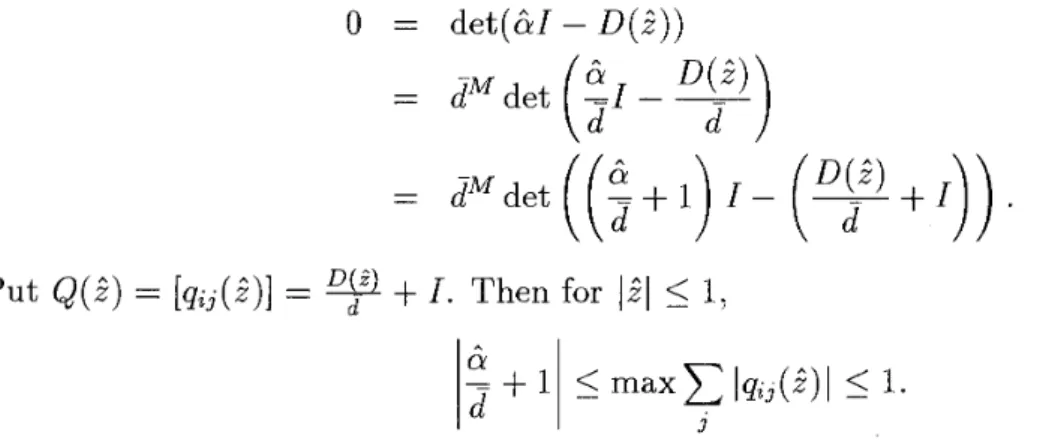
For the existence region of &, we can find as follows. Considering the equation det(&I -

D(?)) = 0, we get

0 = det(&I - D(,?))

(y

+

I)) . Put Q(;) = [qi,(S)] =

+

I . Then for 121

5

1,

Hence we can conclude that & exists at least in

l&

+

d\

<

d.

Since both existence regions of z and a (see Figure 1) are compact, we select a pair of lattice points by suitable intervals in both regions as the initial values of Newton's method to obtain all solutions of (29). A right null vector of z l - A [ z ) is represented by the Kronecker product of right null vectors of al - D ( z ) and z I - h(&). It is proved that in those regions

there are M X N pairs of (i, G), if all zero points of d - A{z) are distinct (see Nishimura and Jiang [l 31).

T h e e x i s t e n c e r e g i o n o f a . T h e e x i s t e n c e r e g i o n o f z.

Figure 1: The existence region of the solutions of (29)

Remark

In general we can not obtain the explicit expression of A(z) because A{z) takes the form as (26). But considering the system of equation (29), we can get zero points of det (z I - ~ ( z ) ) . In a case of N = 1, a M A P / S M / l queue reduces to a M A P / G / l queue. Let H ( t ) be the distribution function of service time with its moment generating function h(a). Then solutions of det ( z I - a ( z ) ) = 0

( 1

zl

5

1) satisfy

where a(z) =

(r

e D w d ~ ( t ) . Therefore, if h,-'(z), the inverse function of z = h(&), exists, we can obtain zero points of det(zI - a(z)) on the unit disk from the equation

(14)

Newton's Method for Zero Points of a Matrix Function

In general, for a M A P / G / l queue, solving the equation

d e t ( a I - D ( h ( a ) ) = _{0 ( \ a}

+

_d\^

_d),

we can obtain all zero points on the unit disk. Especially, for a M A P / D11 queue with a deterministic service time T, h ( a ) =

e07'.

Although h l ( z ) = $ l o g s is not unique, we may solve the equation

d e t ( a I - ~ ( e ~ ~ ) ) = 0 _{( \ a}

+

d\

_<:

_{d ) ,} ₍₃₂₎ and put z = h ( a ) .

3.3. A Superposition of independent Markovian arrival processes

We consider a M A P / G / l queue whose arrival process is a superposition of I{ independent Markovian arrival processes ([3] and [4]). The vth process (U = 1,.

.

,

K ) is formulated

as the M. X M. coefficient matrices {FnlÃ£, = 0 , 1 , .

.

.}. Put FJz) = F n l V ~ " and suppose that F. = F v ( l ) is irreducible and aperiodic. Then the generating function for the arrivals at service completion epochs is given by a(z) =

f^

e D ( z ) t d ~ ( t ) , where H{t) is the distribution function of service time and D(z) Fl(z) Q) F&) @ Fx(z) is a matrix

function for the arrival process. The size of the matrix function D(z) is M X M , where

M =

nf=l

MW. The symbol @ denotes the Kronecker sum of matrices. From the results in

Section 3.2, in order to obtain zero points of det ( z I - a(z)) on the unit disk, we solve the equation

d e t ( a I - D ( h ( a ) ) ) = 0 ( \ a

+

W ) ,

where d is the maximal value of diagonal elements of -Do (Do Fo1 Q)

- -

@ Fo,K)i and put z = h ( a ) . From the property of the Kronecker sum, we get the following theorem.

Theorem 4 Let & be a solution of d e t ( a I - D ( h ( a ) ) = 0 (la

+

d\

<:

d). Then there exists ( a l ,

.

,

a&-) satisfying

a

= al

+

a2

+

.

+

O.K and

1

det (al I - Fl (h(&))) = 0 det ( a J - FIc(h(&))) = 0.

The existence region of a. (v = 1, .

.

,

I() is given by

IQ;(,

+Q

<_ d., where

&,

(v = 1,

. . .

,

K ) is the maximal value of diagonal elements of -Fo,..

Proof. For every v (U = 1,.

.

,

I<), let pi" (i = 1 , .

. .

, M y ) be eigenvalues of Fv(h(&)). According to the same discussion in Theorem 4,

pi.

satisfies

det(&,I - F,(h(&))) = 0 ( i = l , .

. .

,

M,). ₍₃₅₎ Considering Equation (35)) we get

Since lh(&)l

<:

1, the maximum row sum of the absolute value of the entries of the matrix

F" ( h ( & ) )

du

+

I is less than or equal to 1. Therefore

1%

+

11

5

1, that is IDi,,,

+

d.1 $ d..

From the property of the Kronecker sum, & (the eigenvalue of D(h(&)) = Fl(h(&)) Q)

@ Fv(h(&))) is the sum. of eigenvalues of each Fv(h(&)) (v = l , .

.

,

A'). So there exist

(15)

We can apply Theorem 2 to the problem (34). Put a^ = (a?), .

. .

,

n g ) ) and

&W

=

a^

+

- -

+

a^. For f , 7 = 1 , .

. .

,

K ,

let ~ ( ^ ( a ( ~ ) ) be the M( x M( matrix defined by

where ~ : ( h ( & ( ~ ) ) ) = n ~ ~ ( h ( a W ) ) " - l . Then setting

we get the Newton's iteration formula

where ev is the l ' s column vector of size K . The existence region of (v = 1 , . .

.

,

I{) are given by \a,,

+

d u \ <,

&.

4. Numerical Examples

In this section, considering some examples of queueing models, we show results of calculations for zero points by Newton's method and discuss their accuracy and computational times.

(1) A M A P / M / l queue

For a M A P / M / l queue, we now consider to obtain the zero points of det(zI - a(z}} on the unit disk. Let He(t) and h e ( a ) be the exponential distribution of the service time with mean

-1-

and its moment generating function, respectively, that is,

In order to obtain zero points of det(zI - a(z}), from (31) we solve the equation

det ( h i 1 (z) I - D ( z ) ) = det ( ^ l ) ~ - D ( z ) ) = O (lzl

<

1).

z (37)

We consider two cases of M A P / M / 1 queue. In the first case for Newton's method, selecting

initial points on lattice points in the unit disk, we compare the computational time of several size matrices with complex zero points. In the second case, all zero points in the unit disk are real in (0, l]. We compare the accuracy and computational time for Newton's method and those of Lucantoni's method.

(16)

Newton's Method for Zero Points of a Matrix Function 41 1

be the matrix function of size M. Note that this MAP is the same as a Poisson process but this is not an essential assumption. When we use information of range where zero points are distributed, computational times become short. Our aim is to calculate all zero points in the unit disk by selecting all lattice points of the interval S = 0.05 as initial values of Newton's method.

In Table 1, the solutions and corresponding absolute values of det(h;l(z)I - D(z)) are shown when the matrix size of D(z) is 7 X 7.

Table 1: The solutions of det(h;l ( z ) I - D(z)) = 0.

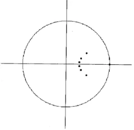
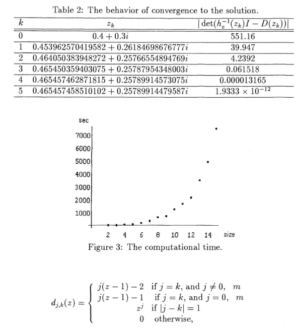
In Figure 2, these zero points are plotted on the complex plane. In Table 2, the behavior of convergence to the solution z = 0.465457458510102

+

0.257899144795876 i is represented with

1

d e t ( h l (zk) I - D(zk))

1

as evaluation of the accuracy. For M = 2, . . . ,15, M distinct

Figure 2: The distribution of the solutions.

zero points are obtained. In general, as the size of D(z) becomes large, the computational time increases. In Figure 3, the computational time is plotted as a function of the size M (CPU: Pentium 166Mhz, Memory: 32MB, OS: Microsoft Windows 95). It takes about 2 hours to calculate all zero points in the case matrix size is 15 X 15 without using information

about zero points. If we can use the knowledge of an region which contains all zero points in the unit disk, we may save the computational time.

The second case. Let {j = 0, , m } be the state space of the underlying process. Suppose that D(z) is an (m

+

1) X (m

+

1) matrix whose (i, j) element (j, k = 0,

,

m) is

(17)

Table 2: The behavior of convergence to the solution. k Z k

1

d e t ( h 2 - D ( 2 k ) )

1

0 0.4

+

0.31 551.16 1 0.453962570419582

+

0.261846986767771 39.947 2 0.464050383948272

+

0.257665548947691 4.2392 sec ~ 0 0 0 1

Figure 3: The computational time.

(

0 otherwise,

where the traffic intensity is p = 3(m

+

l ) x / 2 . Since arrival rate at state j is j, this numerical example possesses burstness of traffic. We will use the following steps. At first decide an interval where zero points are distributed. Next a s initial points of Newton's method select equally spaced 5 m points on the interval.

(i) Comparison of Newton's method and Lucantoni's method when p = 0.5. The results of Newton's method and Lucantoni's method is completely the same. Using both methods

we can get accurate results. In Table 3, computational times of Newton's method and Lucantoni's method are given when p = 0.5 and m = 5,10,15,20. Since in this case all zero points are real, Newton's method is very effective.

Table 3: Computational times (sec)

m 5 10 15 20

Newton's method 1.54 10.61 35.53 116.94

Lucantoni'smethod 160.32 838.16 2525.86 5519.25

(18)

Newton% Method for Zero Points of a Matrix Function 413

method) the calculated G is not stochastic because its row sums are not equal to l. The lowest row sum of the matrix G is 0.959 with 5465.8 second computational time.

On the other hand) in our Newton's method) selecting l00 initial points in the interval [0.87)1], we get all 21 zero points. The smallest zero point is 0.8796392

.. This calculation

is executed during 119 seconds computational time. For Newton's method computational times do not depend on the traffic intensity p. In this heavy traffic case, the calculated matrix G contains negative numbers of order 1op6 by using double precision. Therefore, authors calculate the matrix G by using computer calculations of l000 figures for Decimal BASIC (free ware) made by K. Shiraishi (kazuo.shiraishiQnifty.ne.jp). Then calculated G

becomes stochastic.

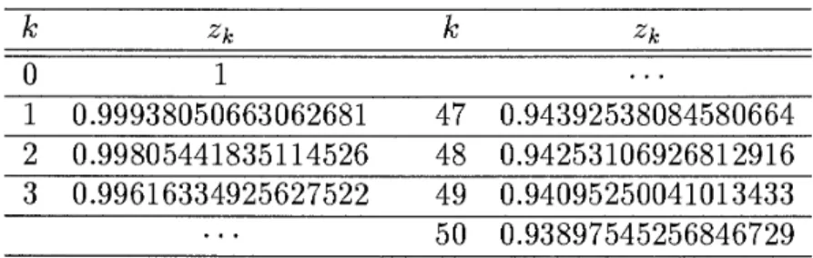
(iii) When m = 50 and p = 0.99, selecting 250 initial points in the interval [0.93)1]) we get all 51 zero points listed in Table 4. Accuracy of zero points is also checked because the calculated matrix G is stochastic. Authors also execute this check by using computer calculations of l000 figures for Decimal BASIC.

Table 4: The list of zero points for m = 50 and p = 0.99.

(2) A M A P / D / l queue

For a M A P / D11 queue, let HD(t) and h D ( a ) be the service time distribution (the service time is T ) and its moment generating function, respectively. Then

In order to obtain zero points of det(zI - a(z)) on the unit disk, from (32) we solve the

equation

d e t ( a I - D ( h D ( a ) ) = d e t ( a I - ~ ( e ~ ~ ) ) = 0 _{( [ a}

+

_dl

₅

_{d ) ,} ₍₃₈₎ where d is the maximum value of diagonal entries of -Do.

Put T =

$

and

r

-1 z2

o

1

Then the solutions of (38) obtained by using Newton's method are 0, -1.1256 - )

-0.95107

+

0.15089 i and -0.95107 - 0.15089 i. Substituting these solutions into z = h D ( a ) , we get zero points. In Table 5) the solutions) their absolute values of d e t ( a I - D(effT)) and corresponding zero points are shown.

(19)

Table 5: The solutions of d e t ( a 1 - D(eaT)) = 0 and their corresponding values of z. ff z

1

d e t ( a I - D(eaT))

1

Q 0 1 -1.1256637738136 - 6.24043216044599 X 10-16i 2.96969 X 10-l7 0.324437043056382 - 2.02462735752905 X 10-16i -0.95107027160039

+

0.150890530571235i 4.44089 X 10-l6 0.381937723896332

+

0.058072184463382~" -0.95107027160039 - 0.150890530571235i 4.44089 X 10-l6 0.381937723896332 - 0.058072184463382i (3) A M A P / S M / l queue

For a M A P / S M / l queue, we consider to solve the equation

d e t ( z I - A(z)) = 0 (121

5

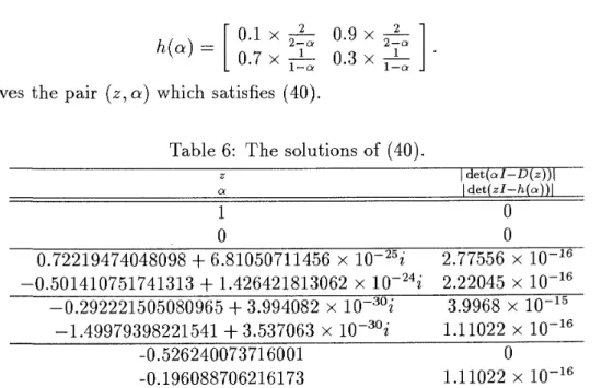
l ) .

As an example, put

To obtain the solution of (39), from Theorem 4 we solve the system of equations

where

Table 6 gives the pair (z, a ) which satisfies (40).

Table 6: The solutions of (40).

z 1 det(a1-D(z))l a 1 det(z1-h(a))l l 0 0 0 0.72219474048098

+

6.81050711456 X 1 0 ~ ~ ~ 2 2.77556 X 10-l6 -0.501410751741313

+

1.426421813062 X 2.22045 X 10-l6 -0.292221505080965

+

3.994082 X 3.9968 X 10-l5 -1.49979398221541

+

3.537063 X l ~ - ~ O i 1.11022 X 10-l6 -0.526240073716001 0 -0.196088706216173 1.11022 X 10-l6

(20)

Newton's Method for Zero Points of a Matrix Function 41 5

5. Conclusions

Comparing direct Newton's method with the method given in Theorem l and 2) the latter has a simpler structure and is executed with less computational time than the former. h a single variable case) the latter computational cost is 0 ( M 3 ) whereas the former is 0 ( M 4 ) .

For a M A P / G / l queueing system) calculation of the matrix G is first important problem. Lucantoni's method is very efficient. But heavy traffic systems, its convergence is slow. We propose the usage of Newton's method to calculate zero points of det(zI - a(z)). There are two problems for usage of Newton's method. The first problem is the assumption that zero points in the unit disk are simple. We can not encounter multiple zero points if we do not make artificial examples. In our numerical examples) all zero points are simple. This assumption seems not t o be so strong in applications. However, it seems that Gail et al.'s method [5] may be aspplied if there are zero points with multiplicity. Second problem is how to select initial points. To save the computational time the following steps are suggested. At the first step) find a restricted region which contains zero points. In authors7 experience this step is not difficult because zero points are distributed in a small region. At the second step) select efficient number of initial points so as to find all zero points in the unit disk) since the number of zero points in the unit disk we need is equal to the size of D(z). Another application of Newton's method is that when we have a roughly approximated matrix G by some method) we may set its eigenvalues as the initial values of Newton's method.

References

N. Akar and K. Sohraby: An invariant subspace approach in M / G / l and G / M / l type Markov chains. Communications in Statistics. Stochastic Models, 13 (1997) 381-416. D. Bini and B. Meini: On the solution of a nonlinear matrix equation arising in queueing problems. SIAM Journal on Matrix Analysis and Applications) 17 (1996) 906-926. A. I. Elwalid and D. Mitra: Effective bandwidth of general Markovian traffic sources and admission control of high speed networks. IEEE Transactions on Networking) l (1993) 329-343.

A. I. Elwalid and D. Mitra: Markovian arrival and service communication systems: spectral expansions separability and Kronecker-product forms. In W. J. Stewart (ed.):

Computations with Markov chain (Kluwer Academic Publisher, 1996)) 507-546.

H. R. Gail) S. L. Hantler and B. A. Taylor: Solutions of the basic matrix equation for M / G / l and G / M / l type Markov chains. Communications in Statistics. Stochastic

Models) I 0 (1994) 1-43.

H. R. Gail, S. L. Hantler and B. A. Taylor: Spectral analysis of M / G / l and G / M / l type Markov chains. Advances in Applied Probability) 28 (1996) 114-1 65.

H.

R.

Gail) S. L. Hantler and B. A. Taylor: Non-skip-free M / G / l and G / M / l type Markov chains. Advances in Applied Probability, 29 (1997) 733-758.

G. Latouche: Newton's iteration for non-linear equations arising in Markov chains. IMA Journal of Numerical Analysis, 14 (1994) 583-598.

D. M, Lucantoni: New results on the single server queue with batch Markovian arrival process. Communications in Statistics. Stochastic Models) 7 (1991) 1-41.

I. Mitrani: The spectral expansion solution method for Markov processes on lattice strips. In J. H. Dshalalow (ed.) Advances in Queueing (CRC Press) Inc, Florida) 1995)) 337-352. ,

(21)

[ll] M. F. Neuts: Structured Stochastic Matrices of M / G / l Type and Their Applications. (Marcel Dekker Inc) New York7 1989).

[l21 S. Nishimura: Eigenvalue expression for a batch Markovian arrival process. Asia-Pacific Journal of Operational Research, 15 (1998) 193-202.

[l31 S. Nishimura and Y. Jiang: Spectra of matrix generating function for a MAP/SM/l queue. Communications in Statistics. Stochastic Models) 16 (2000) 99-120.

[l41 S. Nishimura and H. Sato: Eigenvalue expression for a batch Markovian arrival process. Journal of the Operations Research Society of Japan) 40 (1997) 122-132.

[l51 V* Ramaswami: A stable recursion for the steady state vector in Marlcov chains of M / G / l type. Communications in Statistics. Stochastic Models) 4 (1988) 183-188.

S hoichi Nishimura

Depart~nent of Applied Mathematics Science University of Tokyo

1-3 Kagurazaka) Shinjuku-ku) Tokyo, Japan nishimur@rs. kagu. sut

.

ac. J P

At sushi Harasliima Mitsuba Co.