Vol. 53, No. 2, June 2010, pp. 119–135
CORRELATED MULTIVARIATE SHOCK MODELS ASSOCIATED WITH A RENEWAL SEQUENCE AND ITS APPLICATION TO ANALYSIS OF
BROWSING BEHAVIOR OF INTERNET USERS
Ushio Sumita Jinshui Zuo
University of Tsukuba
(Received July 29, 2009; Revised January 22, 2010)
Abstract A correlated multivariate shock model is considered where a system is subject to a sequence of J different shocks triggered by a common renewal process. Let (Y (k))∞k=1 be a sequence of inde-pendently and identically distributed (i.i.d.) nonnegative random variables associated with the renewal process. For the magnitudes of the k-th shock denoted by a random vector X(k), it is assumed that [X(k), Y (k)] (k = 1, 2,· · · ) constitute a sequence of i.i.d. random vectors with respect to k while X(k) and
Y (k) may be correlated. The system fails as soon as the historical maximum of the magnitudes of any
component of the random vector exceeds a prespecified level of that component. The Laplace transform of the probability density function of the system lifetime is derived, and its mean and variance are obtained explicitly. Furthermore, the probability of system failure due to the i-th component is obtained explicitly for all i∈ J = {1, · · · , J}. The model is applied for analyzing the browsing behavior of Internet users.
Keywords: Applied probability, multivariate shock models, system lifetime, consumer
browsing behavior
1. Introduction
A general shock model is studied by Shanthikumar and Sumita [3], where a system is sub-ject to a sequence of random shocks generated by a renewal sequence. More specifically, the model is characterized by correlated pairs of nonnegative random variables [Xj, Yj] (j =
1, 2,· · · ) where Xj is the magnitude of the jth shock and Yj describes the time interval
between two consecutive shocks. The variates [Xj, Yj] (j = 1, 2,· · · ) are i.i.d. pairwise,
while Xj and Yj may be correlated. The underlying system fails as soon as the magnitude
of a shock exceeds a prespecified level. The transform results, an exponential limit theorem and properties of the associated renewal processes of the system failure times are obtained with an application to a stochastic clearing system. The model is extended subsequently by Sumita and Shanthikumar [4] to incorporate the system lifetime based on the cumulative shock.
While the general shock model has widened the application areas much beyond the tra-ditional Poisson shock model, it is still limited in that the model accepts only one type of shocks. In some applications, it is important to deal with multiple types of shocks generated by a common renewal sequence. In analyzing the browsing behavior of users of the Internet, for example, it is common to find a user moving from one website to another in order to gather information about a specific product of his/her interest. Assuming that dwell times at different websites constitute a renewal sequence, the first type of shocks may correspond to the values of information gathered from various websites concerning a product produced by Company C1, while the second type of shocks may describe those concerning a similar
product produced by Company C2. The Internet search would be terminated when the user obtains enough information to decide which company’s product should be purchased. The purpose of this paper is to extend the general shock model of Shanthikumar and Sumita [3] so as to incorporate such multiple different random shocks generated from a common re-newal sequence. A preliminary version of this study is reported at IWAP2008 by Sumita and Zuo [5]. In this paper, however, the model analysis is elaborated further substantially. In particular, analysis of the probability of system failure due to the i-th component is totally new and numerical examples are also enriched. It may be worth noting that the proposed model can be interpreted as a fatal shock model, where the fatal shock is defined as the historical maximum of any component of a sequence of random vectors exceeding a pre-specified level for the component.
The structure of this paper is as follows. The correlated multivariate shock model is introduced in Section 2 and the system lifetime is analyzed in Section 3. In Section 4, the probability of system failure due to component i is evaluated explicitly. An application to analysis of the browsing behavior of users of the Internet is discussed in Section 5, and numerical examples are also presented. Finally, in Section 6, some concluding remarks are given.
2. Model Description
We consider a system where a sequence of J different types of shocks are triggered by a common renewal process characterized by a sequence of i.i.d. nonnegative random variables (Y (k))∞k=1. Let X(k) = [X1(k),· · · , XJ(k)] be the random vector describing the magnitudes
of J different shocks occurred at the k-th renewal epoch. Throughout the paper, we assume that all random variables are absolutely continuous with X(k)∈ RJ+and Y (k)∈ R+, where
RJ
+ is the set of J dimensional nonnegative vectors and R+ denotes the set of nonnegative real numbers. For notational convenience, we define J = {1, 2, , · · · , J} and its power set B(J ) = {A : A ⊂ J }. In addition, while X(k) and Y (k) may be correlated, it is assumed that [X(k), Y (k)] (k = 1, 2,· · · ) constitute a sequence of i.i.d. random vectors with respect to k. The joint distribution function and the joint probability density function of [X(k), Y (k)] are defined by FX,Y(x, y) = P [X1(k) < x1,· · · , XJ(k) < xJ, Y (k) ≤ y], (2.1) and FX,Y(x, y) = ∫ xJ 0 · · · ∫ x1 0 ∫ y 0 fX,Y(v, w)dwdv. (2.2)
We note that the inequality associated with X(k) in FX,Y(x, y) is taken to be strict. Since
the historical maximum processes are of our main concern, equalities are attached to tail probabilities for random variables directly involving X(k) as a general rule in this paper. For notational convenience, the following functions are also introduced.
fY(y) = ∫ ∞ 0 · · · ∫ ∞ 0 fX,Y(x, y)dx ; fX(x) = ∫ ∞ 0 fX,Y(x, y)dy (2.3) GX(x, y) = ∫ xJ 0 · · · ∫ x1 0 fX,Y(v, y)dv (2.4) GX(x, y) = ∫ ∞ xJ · · · ∫ ∞ x1 fX,Y(v, y)dv (2.5)
GY(x, y) = ∫ y 0 fX,Y(x, τ )dτ ; GY(x, y) = ∫ ∞ y fX,Y(x, τ )dτ. (2.6)
For simplicity, with x = [x1,· · · , xJ], we write fX(x) = fX(x1,· · · , xJ), GX(x, y) =
GX(x1,· · · , xJ, y), etc, interchangeably.
The system fails as soon as the historical maximum of the magnitudes of any component of the random vector exceeds a prespecified level of that component. More specifically, let
N (t) be the counting process associated with the renewal sequence (Y (k))∞k=1 and define the historical maximum process M (t) by
M (t) = [M1(t),· · · , MJ(t)] ; Mi(t) = max
0≤k≤N(t){Xi(k)}, (2.7) where X(0) = 0 is employed for notational convenience. The system fails as soon as any one of the historical maximum processes Mi(t), i ∈ J , exceeds its prespecified level zi .
If only Mi(t) exceeds zi, then the i-th component causes the system failure. If multiple
historical maximum processes exceed their prespecified levels simultaneously, the system failure is assumed to be triggered by the component having the largest value of them. For
z = [z1,· · · , zJ] > 0, the system lifetime Tz is then given by
Tz = inf{t : Mi(t)≥ zi, for some i∈ J }. (2.8)
Of interest is the distribution of Tz and the probability ρi(z) of the system failure being
caused by the i-th component. In what follows, we analyze Tz, deriving the transform results
and its mean and variance, as well as ρi(z) for all i∈ J .
3. Analysis of Tz
Let the distribution functions of M (t) and Tz be defined by
V (z, t) = P [M (t) < z] ; Wz(t) = P [Tz ≤ t]. (3.1)
Laplace transforms with respect to t are denoted by a circumflex, i.e., ˆ V (z, s) = ∫ ∞ 0 e−stV (z, t)dt ; wˆz(s) = ∫ ∞ 0 e−stdWz(t). (3.2)
One easily sees that there exists a dual relationship between M (t) and Tz specified by
V (z, t) = P [M (t) < z] = P [Tz > t] = Wz(t), (3.3)
where Wz(t) = 1− Wz(t) is the survival function of Tz. In this section, we derive ˆwz(s)
explicitly based on Equation (3.3).
We assume that the system starts anew at time t = 0. For k = 1, 2,· · · , the shock vector
X(k) at the k-th renewal epoch is correlated only to the time interval Y (k) since the (k−1)st
renewal epoch and does not affect the future events. The following theorem then holds.
Theorem 3.1. Let ˆϕY(s) and ˆGX(z, s) be the Laplace transforms of fY(t) in Equation (2.3)
and ˆGX(z, s) in Equation (2.6) respectively, i.e. ˆϕY(s) def
= ∫0∞e−stfY(t)dt and ˆGX(z, s) def
= ∫∞
0 e−stGX(z, t)dt. One then has ˆ
V (z, s) = 1− ˆϕY(s) s{1 − ˆGX(z, s)}
Proof. Since V (z, t) is the probability that the maximum value of Xi(k) has not exceeded
the level zi for k = 1, 2,· · · , N(t) and i ∈ J , by conditioning on the first renewal time Y (1)
and using the regenerative property of the paired process [X(k), Y (k)] at Y (1), one sees that
V (z, t) = FY(t) +
∫ t
0
GX(z, y)V (z, t− y)dy. (3.4)
By taking the Laplace transform of both sides of Equation (3.4) with respect to t, it can be seen that
ˆ
V (z, s) = 1− ˆϕY(s)
s + ˆGX(z, s) ˆV (z, s).
This equation can be solved for ˆV (z, s), completing the proof.
The system lifetime Tz has the dual relationship with M (t) given in Equation (3.3). The
Laplace transform ˆwz(s) = E[e−sTz] is then easily found from Theorem 3.1.
Theorem 3.2. ˆ wz(s) = ˆ ϕY(s)− ˆGX(z, s) 1− ˆGX(z, s) , Re(s)≥ 0.
Proof. From Equation (3.3), one finds that ˆV (z, s) = 1− ˆwz(s)
s , so that ˆwz(s) = 1− s ˆV (z, s).
The theorem now follows from Theorem 3.1.
By differentiating ˆwz(s) at s = 0, the mean and the variance of Tz can be obtained.
Corollary 3.2.1. a) E[Tz] = E[Y ] 1− FX(z) b) V ar[Tz] = E[Y2] 1− FX(z) + E[Y ] (1− FX(z))2 { 2FX(z)E[Y|X < z] − E[Y ] }
The Laplace transform ˆwz(s) = E[e−sTz] has the following real-domain form.
wz(t) = fY(t) + ∞ ∑ k=1 fY(t)∗ G (k) X (z, t)− ∞ ∑ k=1 G(k)X (z, t), (3.5) where G(k+1)X (z, t) = ∫0tGX(z, t−τ)G (k)
X (z, τ )dτ and the asterisk denotes similar convolution
in t.
As the threshold levels zi for i ∈ J tend to approach ∞, the system failure becomes a
rare event. Accordingly, it may be expected that Tz/E[Tz] converges in distribution to the
exponential variate E of mean one. This type of exponential limit theorems is originated from Keilson [1, 2] involving rare events in regenerative processes. Since the historical max-imum is monotonically non-decreasing in time t, Keilson’s theorem does not seem to be directly applicable here. However, Shanthikumar and Sumita [3] find the structural similar-ity between rare events in regenerative processes and those in historical maximum processes,
proving a generalized version of the original theorem by Keilson [1, 2].
The limit theorem of [3] involves a sequence of non-negative random vectors V (k) = [X(k), Y (k)] where X(k) and Y (k) may be correlated but V (k)’s are i.i.d. Then the state space N = R2
+ ={(x, y) : x ≥ 0, y ≥ 0} is decomposed into G(z) and B(z) with G(z) 6= ∅,
B(z)6= ∅, G(z) ∩ B(z) = ∅ and G(z) ∪ B(z) = N , and the following experiment is
consid-ered. If V (k) ∈ G(z), the experiment continues and V (k + 1) is chosen. The experiment stops when a random vector falls in the region B(z). The system failure time Sz is then
defined as the sum of y-coordinates of all random vectors up to the stopping point. It is shown in Shanthikumar and Sumita [3] that, if pz = P [V ∈ B(z)] → 0 as z → ∞, then
Sz/E[Sz]→ E as z → ∞. In this paper, one has V (k) = [X(k), Y (k)], i.e. the first process
becomes multivariate. This requires to redefine N , G(z), B(z) and pz. However, the system
failure time remains to be expressed as the sum of y-coordinates of all random vectors up to the stopping point in the random experiment. Since pz = P [V (k)∈ B(z)] → 0 if zi → ∞
for all i ∈ J , the following theorem can be shown along the line of the proof of Theorem 1.A4 in [3].
Theorem 3.3. Let E be the exponential random variate of mean one and suppose 0 < FX,Y(x, y) < 1 for 0 < x < ∞, 0 < y < ∞, and E[Y ] < ∞. Then Tz/E[Tz]
d
→ E as z → ∞.
It is trivial that the almost sure dominance of Tz2 over Tz1 is present whenever 0≤ z1 ≤
z2. We formally state this result.
Theorem 3.4.
0≤ z1 ≤ z2 ⇒ Tz1 ≤a.s.Tz2
4. Probability of System Failure Caused by the i-th Component
Given a threshold vector z, we next turn our attention to evaluate the probability ρi(z)
of system failure caused by the i-th component for i ∈ J . For this purpose, let τk be the
k-th renewal epoch for k = 1, 2,· · · and define ηJ(z, t, k) to describe the event that the system failure is avoided at the k-th renewal epoch with the marginal probability density of t at t = τk. Since [X(k), Y (k)] constitute a sequence of i.i.d. random vectors, ηJ(z, t, 1)
represents the avoidance of system failure at any single renewal epoch. It can be seen that
ηJ(z, t) def= ηJ(z, t, 1) = d dtFX,Y(z, t) = ∫ zJ 0 · · · ∫ z1 0 fX,Y(x, t)dx1· · · dxJ. (4.1)
For k≥ 2, one sees that
ηJ(z, t, k) def= d
dtP [Xi(m) < zi for all i∈ J and m = 1, · · · , k, τk ≤ t]
= ∫ t
0
ηJ(z, τ, k− 1)ηJ(z, t− τ)dτ. (4.2)
By taking Laplace transforms of Equations (4.1) and (4.2) with respect to t, one finds by induction that ˆ ηJ(z, s, k) = ∫ ∞ 0 e−stηJ(z, t, k)dt ={ˆηJ(z, s)}k, k = 1, 2,· · · , (4.3)
where ˆ ηJ(z, s) = ∫ ∞ 0 e−stηJ(z, t)dt. (4.4)
LetFi(J ) be the family of subsets of J containing i, that is,
Fi(J )
def
= {A : i ∈ A, A ⊂ J }, (4.5)
and define ηi:A,J \A(z, t, k) to be the probability that the system failure is triggered by the
i-th component and all the components in A ∈ Fi(J ) exceed the corresponding threshold
levels at the k-th renewal epoch while Xj(k) for j ∈ J \A remains below zj, with the
marginal probability density of t at t = τk. More specifically, we define, for k ≥ 2,
ηi:A,J \A(z, t, k) def
= d
dtP [Xi(m) < zi for all i∈ J and m = 1, · · · , k − 1, and (4.6) Xj(k) > zj for j ∈ A, Xj(k) < zj for j ∈ J \A, Xi(k) = max
j∈A{Xj(k)}, τk≤ t].
For k = 1, the first half of the conditions in the above probability would be ignored, i.e
ηi:A,J \A(z, t, 1) (4.7)
def
= d
dtP [Xj(1) > zj for j ∈ A, Xj(1) < zj for j ∈ J \A, Xi(1) = maxj∈A{Xj(1)}, τ1 ≤ t].
As before, since [X(k), Y (k)] are i.i.d. random vectors, ηi:A,J \A(z, t, 1) represents a system failure at any single renewal epoch with the probability density of the renewal lifetime being at t. It can be seen that, with ηi:A,J \A(z, t)def= ηi:A,J \A(z, t, 1), and for k≥ 2,
ηi:A,J \A(z, t, k) = ∫ t
0
ηJ(z, τ, k− 1)ηi:A,J \A(z, t− τ)dτ. (4.8) Adding ηi:A,J \A(z, t, k) over A∈ Fi(J ), one obtains the probability that the system failure
is triggered by the i-th component at the k-th renewal epoch with the marginal probability density of t at t = τk . We define ξi(z, t) def = ξi(z, t, 1) def = ∑ A∈Fi(J ) ηi:A,J \A(z, t), (4.9) and ξi(z, t, k) def = ∑ A∈Fi(J ) ηi:A,J \A(z, t, k). (4.10)
It then follows from Equations (4.8) through (4.10) that, for k≥ 2,
ξi(z, t, k) =
∫ t
0
Let the Laplace transform of ξi(z, t) with respect to t be defined by ˆ ξi(z, s) def = ∫ ∞ 0 e−stξi(z, t)dt. (4.12)
From Equations (4.3) and (4.11), one then has, for k≥ 2, ˆ ξi(z, s, k) def = ∫ ∞ 0 e−stξi(z, t, k)dt ={ˆηJ(z, s)}k−1ξˆi(z, s). (4.13)
We note that this Laplace transform result is valid even for k = 1, yielding the definition ˆ
ξi(z, s, 1) = ˆξi(z, s). The corresponding Laplace transform generating function can then be
obtained as ˆ ˆ ξi(z, s, u) def = ∞ ∑ k=1 ˆ ξi(z, s, k)uk= u· ˆξi(z, s) 1− u · ˆηJ(z, s). (4.14)
We are now in a position to state the main theorem of this section.
Theorem 4.1. Given a threshold level vector z, let ρi(z) be the probability that the system
failure is eventually caused by the i-th component. Then one has ρi(z) =
∫∞
0 ξi(z, t)dt
1−∫0∞ηJ(z, t)dt. (4.15)
Proof. Since ρi(z) =ξˆˆi(z, 0, 1), the theorem follows immediately from Equation (4.14).
Remark 4.2. In e-commerce, the probability ρi(z) that Product i is chosen to be purchased
over Product j, j ∈ J \ {i}, represents the strength of Product i against other competitive products. If the brand power of Product i is strong, customers would not require much information about Product i. This means that a smaller value of zi is likely to convince
customers to purchase. Given zi, if the website of Product i is well organized, it is likely to
enable customers to reach zi sooner. Consequently, one may expect that ρi(z) increases as
zi decreases or Xi increases stochastically. It is non-trivial to prove this conjecture based on
Theorem 4.1. However, we will demonstrate this conjecture through numerical examples.
In Theorem 4.1, the denominator of ρi(z) can be computed rather easily from Equation
(4.1). As can be seen from Equation (4.15), the numerator, however, requires the summation over A∈ Fi(J ) which grows exponentially as a function of J. Accordingly, it is not easy to
compute the numerator when J is large. If the threshold level of each component is identical, i.e. z = z1 where 1 is the vector having all components equal to 1, the computation of the numerator can be simplified significantly. Namely, one has
ξi(z1, t) = d dtP [Xi(1) = maxj∈J {Xj(1)} > z, τ1 ≤ t] = ∫ ∞ z dxi ∫ xi1\i 0\i fX,Y(x, t)dx, (4.16)
where a\idef= [a1,· · · , ai−1, ai+1,· · · , aJ]T.
WhenJ = {1, 2}, the summation over A ∈ Fi(J ) can be written explicitly, enabling one
to evaluate ρi(z1, z2). More specifically, one has
ξ1(z1, z2, t) = η1,2(z1, z2, t) + η1:1,2(z1, z2, t) (4.17) ξ2(z1, z2, t) = η1,2(z1, z2, t) + η2:1,2(z1, z2, t) (4.18) where η1,2(z1, z2, t) = ∫ z2 0 ∫ ∞ z1 fX,Y(x1, x2, t)dx1dx2 ; (4.19) η1,2(z1, z2, t) = ∫ ∞ z2 ∫ z1 0 fX,Y(x1, x2, t)dx1dx2 ; (4.20) and η1:1,2(z1, z2, t) def = d dtP [X1(1)≥ z1, X2(1)≥ z2, X1(1) > X2(1), τ1 ≤ t] ; (4.21) η2:1,2(z1, z2, t) def = d dtP [X1(1)≥ z1, X2(1)≥ z2, X1(1) < X2(1), τ1 ≤ t]. (4.22)
When z1 > z2, Equations (4.21) and (4.22) are given by
η1:1,2(z1, z2, t) = ∫ ∞ z1 [ ∫ x1 z2 fX,Y(x1, x2, t)dx2 ] dx1 ; (4.23) η2:1,2(z1, z2, t) = ∫ ∞ z1 [ ∫ x2 z1 fX,Y(x1, x2, t)dx1 ] dx2. (4.24)
For z1 ≤ z2, one has
η1:1,2(z1, z2, t) = ∫ ∞ z2 [ ∫ x1 z2 fX,Y(x1, x2, t)dx2 ] dx1 ; (4.25) η2:1,2(z1, z2, t) = ∫ ∞ z2 [ ∫ x2 z1 fX,Y(x1, x2, t)dx1 ] dx2. (4.26)
The results in Equations (4.17) through (4.26) will be used for numerical examples to be presented in the next section.
5. Application to Analysis of the Browsing Behavior of Users of the Internet
We suppose that a consumer visits various websites in order to gather information about two products of the same type. Let X1(k) be the value of information about the product
P 1 of Company C1 that the consumer gains from the k-th search with length of Y (k), and X2(k) is defined similarly for the product P 2 of Company C2. We assume that both X1(k) and X2(k) consist of two parts: a part independent of Y (k) and another part proportional to
Y (k). The former parts for X1(k) and X2(k) are denoted by ˆX1(k) and ˆX2(k) respectively. They may represent the amount of information about P 1 and that about P 2 that can be gathered from websites, having information about both P 1 and P 2. The number of websites
with P 1 information only may not be necessarily the same as the number of websites with
P 2 information. If the ratio between the two numbers is given as α1 : α2, the amount of information about P i gathered from such websites during search time Y (k) may be written as αiY (k) for i∈ {1, 2}. More formally, we define
X1(k) = Xˆ1(k) + α1Y (k) ; X2(k) = ˆX2(k) + α2Y (k). (5.1) It is assumed that ˆX1(k), ˆX2(k) and Y (k) constitute three independent renewal sequences with respect to k, but X1(k) and X2(k) are not independent because of sharing the common value of Y (k).
Let FX,Y(x1, x2, y) = P [X1(k) < x1, X2(k) < x2, Y (k) ≤ y], and let the distribution functions of ˆX1 and ˆX2 be denoted by FX1ˆ (x) and FX2ˆ (x) respectively. From Equation (5.1), by conditioning on Y , one finds that
FX,Y(x1, x2, y) =
∫ min{y,x1 α1,x2α2} 0
FX1ˆ (x1− α1τ )FX2ˆ (x2− α2τ )fY(τ )dτ. (5.2)
From Equation (2.2), it then follows that
fX,Y(x1, x2, y) = fX1ˆ (x1− α1y)fX2ˆ (x2− α2y)fY(y)· I{0 ≤ y ≤ min{
x1
α1
,x2 α2}},
(5.3)
where I{ST } = 1 if statement ST is true, I{ST } = 0 otherwise. We assume that ˆX1(k), ˆ
X2(k) and Y (k) are exponentially distributed with respective probability density functions given by
fX1ˆ (ˆx1) = µ1e−µ1x1ˆ ; fX2ˆ (ˆx2) = µ2e−µ2ˆx2; fY(y) = λe−λy. (5.4)
Suppose that the consumer will stop the search process whenever the desired information for either product, specified by z1 or z2, is obtained. Let γ∗ and γ∗ be defined as
γ∗ def= min{z1 α1 , z2 α2 } ; γ∗ def= max{z1 α1 , z2 α2 }, (5.5)
and let A(s), B(s), C(s) and D(s) be given by
A(s) = λe −µ1z1(1− e−(s+λ−µ1α1)γ∗) s + λ− µ1α1 ; B(s) = λe −µ2z2(1− e−(s+λ−µ2α2)γ∗) s + λ− µ2α2 C(s) = λe −(µ1z1+µ2z2)(1− e−(s+λ−µ1α1−µ2α2)γ∗) s + λ− µ1α1− µ2α2 ; D(s) = λe −(s+λ)γ∗ s + λ . (5.6)
Then from Theorem 3.2 and Equations (5.1) through (5.6), one has the following theorem.
Theorem 5.1. Let Tz be the web search completion time as defined in Equation (2.8). Then
its Laplace transform is given by
ˆ wz(s) = { 1 + s s+λ A(s) + B(s)− C(s) + D(s) }−1 .
Proof. From Equations (5.2) through (5.4), one has
fX,Y(x1, x2, y) = µ1e−µ1(x1−α1y)µ2e−µ2(x2−α2y)λe−λyI{0 ≤ y ≤ min(
x1
α1
,x2 α2
)}. For notational convenience, let
˜
fX,Y(x1, x2, y) def
= µ1e−µ1(x1−α1y)µ2e−µ2(x2−α2y)λe−λy. (5.7) It can be seen that
GX,Y(z1, z2, y) = ∫ z2 0 { ∫ z1 0 fX,Y(x1, x2, y)dx1 } dx2 = ∫ z2 0 { ∫ z1 0 ˜ fX,Y(x1, x2, y)I{α1y≤ x1 ≤ α1 α2 x2 ≤ z1}dx1 + ∫ z1 0 ˜ fX,Y(x1, x2, y)I{α1y ≤ x1 ≤ z1 ≤ α1 α2 x2}dx1 + ∫ z1 0 ˜ fX,Y(x1, x2, y)I{α1y ≤ α1 α2 x2 ≤ x1 ≤ z1}dx1 } dx2, which leads to GX,Y(z1, z2, y) = ∫ z2 0 [ ∫ α1 α2x2 α1y ˜ fX,Y(x1, x2, y)dx1I{α1y≤ α1 α2 x2 ≤ z1} + ∫ z1 α1y ˜ fX,Y(x1, x2, y)dx1I{α1y≤ z1 ≤ α1 α2 x2} + ∫ z1 α1 α2x2 ˜ fX,Y(x1, x2, y)dx1I{α1y≤ α1 α2 x2 ≤ z1} ] dx2.
Since the first term and the third term in the last part of the above equation can be combined as a single integral from α1y to z1, one finds that
GX,Y(z1, z2, y) = ∫ z2 0 [ ∫ z1 α1y ˜ fX,Y(x1, x2, y)dx1 { I{α1y ≤ z1 ≤ α1 α2 x2} + I{α1y≤ α1 α2 x2 ≤ z1} }] dx2. Substituting Equation (5.7) into the above equation, one has
GX,Y(z1, z2, y) = λe−(λ−µ1α1−µ2α2)y[e−µ1α1y − e−µ1z1]
× ∫ z2 0 µ2e−µ2x2 { I{α2y≤ α2 α1 z1 ≤ x2} + I{α2y ≤ x2 ≤ α2 α1 z1} } dx2. By repeating this procedure with respect to x2, one concludes that
GX,Y(z1, z2, y) = {
e−(µ1z1+µ2z2)λe−(λ−µ1α1−µ2α2)y− e−µ1z1λe−(λ−µ1α1)y
−e−µ2z2λe−(λ−µ2α2)y + λe−λy }
where γ∗ def= min{α1z1,α2z2} is as in Equation (5.5). By taking the Laplace transform of both
sides of Equation (5.8) with respect to y, it follows that ˆ GX,Y(z1, z2, s) def = ∫ ∞ 0
e−syGX,Y(z1, z2, y)dy
= λe −(µ1z1+µ2z2) s + λ− µ1α1− µ2α2 (1− e−(s+λ−µ1α1−µ2α2)γ∗)− λe −µ1z1 s + λ− µ1α1 (1− e−(s+λ−µ1α1)γ∗) − λe−µ2z2 s + λ− µ2α2 (1− e−(s+λ−µ2α2)γ∗) + λ s + λ(1− e −(s+λ)γ∗ ). Since ϕY(s) def = ∫ ∞ 0
e−syλe−λydy = λ s + λ,
one sees that,
ϕY(s)− ˆGX,Y(z1, z2, s) = λe −µ1z1 s + λ− µ1α1 (1− e−(s+λ−µ1α1)γ∗) + λe −µ2z2 s + λ− µ2α2 (1− e−(s+λ−µ2α2)γ∗) − λe−(µ1z1+µ2z2) s + λ− µ1α1− µ2α2 (1− e−(s+λ−µ1α1−µ2α2)γ∗) + λ s + λe −(s+λ)γ∗ , and 1− ˆGX,Y(z1, z2, s) = λe −µ1z1 s + λ− µ1α1 (1− e−(s+λ−µ1α1)γ∗) + λe −µ2z2 s + λ− µ2α2 (1− e−(s+λ−µ2α2)γ∗) − λe−(µ1z1+µ2z2) s + λ− µ1α1− µ2α2 (1− e−(s+λ−µ1α1−µ2α2)γ∗) + s + λe −(s+λ)γ∗ s + λ .
With A(s), B(s), C(s) and D(s) as defined in Equation (5.6), it can be seen that
ˆ wz(s) = ˆ ϕY(s)− ˆGX(z, s) 1− ˆGX(z, s) = { 1 + s s+λ A(s) + B(s)− C(s) + D(s) }−1 ,
completing the proof.
For this example, E[Tz] can be evaluated explicitly from Corollary 3.2.1, as depicted in
Figure 1. We note that the monotonicity of E[Tz] in z can be observed.
The probability of Product i being purchased can be derived directly from Equations (4.16) through (4.25) and Theorem 4.1. Let γ∗, γ∗ and A(s), B(s), C(s) and D(s) be as in Equations (5.5) and (5.6) respectively. One then has the following theorem. Proof is rather mechanical and is omitted here.
Theorem 5.2. The probability of Product i being purchased can be evaluated through the four cases below:
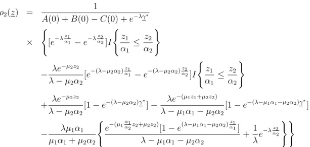
Figure 1: Mean search time ( µ1 = 2.7, µ2 = 2.7, α1 = 0.2, α2 = 0.1, λ = 6 ) Case 1: z1 > z2, α1 > α2 ρ1(z) = 1 A(0) + B(0)− C(0) + e−λγ∗ × {{[e−λα1z1 − e−λα2z2]− λe −µ2z2 λ− µ2α2 [e−(λ−µ2α2)α1z1 − e−(λ−µ2α2)α2z2] } I { z1 α1 ≤ z2 α2 } + λe −µ1z1 λ− µ1α1 [1− e−(λ−µ1α1)γ∗]− λe −(µ1z1+µ2z2) λ− µ1α1 − µ2α2 [1− e−(λ−µ1α1−µ2α2)γ∗] +[e−(µ1z1+µ2z2)− µ1 µ1+ µ2 e−(µ1z1+µ2z1)]λ[1− e −(λ−µ1α1−µ2α2)γ∗] λ− µ1α1− µ2α2 + λe −µ2z2 λ− µ2α2 [e−(λ−µ2α2)z1α1 − e−(λ−µ2α2)α2z2]I { z1 α1 ≤ z2 α2 } − µ1 µ1+ µ2 ·λ[e−(λ−µ2 α2+µ2α1)α1z1 − e−(λ−µ2α2+µ2α1)α2z2 ] λ− µ2α2+ µ2α1 I { z1 α1 ≤ z2 α2 } − λe−µ1z1 λ− µ1α1 [e−(λ−µ1α1)α2z2 − e−(λ−µ1α1)α2z1]I { z2 α2 ≤ z1 α1 } −µ1λe−(µ1z1+µ2z2) µ1+ µ2 · [e−(λ−µ1α1−µ2α2)α2z2 − e−(λ−µ1α1−µ2α2)α1z1] λ− µ1α1− µ2α2 I { z2 α2 ≤ z1 α1 } +e−λγ∗ +λe −(λ−µ2α2+µ2α1)γ∗ λ− µ2α2+ µ2α1 }
ρ2(z) = 1 A(0) + B(0)− C(0) + e−λγ∗ × { λe−µ2z2 λ− µ2α2 [1− e−(λ−µ2α2)γ∗]− λe −(µ1z1+µ2z2) λ− µ1α1− µ2α2 [1− e−(λ−µ1α1−µ2α2)γ∗] + { [e−λα2z2 − e−λα1z1]− λe −µ1z1 λ− µ1α1 [e−(λ−µ1α1)z2α2 − e−(λ−µ1α1)α1z1] } +µ1λe −(µ1+µ2)z1 µ1+ µ2 · 1− e−(λ−µ1α1−µ2α2)α1z1 λ− µ1α1− µ2α2 + µ1λ µ1+ µ2 · e−(λ−µ2α2+µ2α1)α1z1 λ− µ2α2+ µ2α1 } Case 2: z1 ≤ z2, α1 > α2, ρ1(z) = 1 A(0) + B(0)− C(0) + e−λγ∗ × { [e−λα1z1 − e−λα2z2]− λe −µ2z2 λ− µ2α2 [e−(λ−µ2α2)α1z1 − e−(λ−µ2α2)z2α2] + λe −µ1z1 λ− µ1α1 [1− e−(λ−µ1α1)γ∗]− λe −(µ1z1+µ2z2) λ− µ1α1− µ2α2 [1− e−(λ−µ1α1−µ2α2)γ∗] + λµ2α2 µ1α1 + µ2α2 · { e−(µ1α1α2z2+µ2z2) [1− e(λ−µ1α1−µ2α2)α2z2 ] λ− µ1α1− µ2α2 + 1 λe −λz2 α2 }} ρ2(z) = 1 A(0) + B(0)− C(0) + e−λγ∗ × { λe−µ2z2 λ− µ2α2 [1− e−(λ−µ2α2)γ∗]− λe −(µ1z1+µ2z2) λ− µ1α1− µ2α2 [1− e−(λ−µ1α1−µ2α2)γ∗] + { [e−λα2z2 − e−λ z1 α1]− λe −µ1z1 λ− µ1α1 [e−(λ−µ1α1)α2z2 − e−(λ−µ1α1) z1 α1] } +λ[e −µ1z1 − µ2 µ1+µ2e −(µ1+µ2)z1][1− e−(λ−µ1α1−µ2α2)α1z1] λ− µ1α1− µ2α2 +λe −µ2z2[e−λ−µ2α2)α1z1 − e−(λ−µ2α2)z2α1 ] λ− µ2α2 − µ2 µ1+ µ2 · λe−(µ1+µ2)z2[e−(λ−µ1α1−µ2α2 )z1 α1 − e−(λ−µ1α1−µ2α2) z2 α1] λ− µ1α1− µ2α2 + µ1 µ1+ µ2 · λe−(λ−µ2α2+µ2α1)α1z2 λ− µ2α2+ µ2α1 }
Case 3: z1 > z2, α1 ≤ α2, ρ1(z) = 1 A(0) + B(0)− C(0) + e−λγ∗ × { λe−µ1z1 λ− µ1α1 [1− e−(λ−µ1α1)γ∗]− λe −(µ1z1+µ2z2) λ− µ1α1− µ2α2 [1− e−(λ−µ1α1−µ2α2)γ∗] + { [e−λα1z1 − e−λα2z2]− λe −µ2z2 λ− µ2α2 [e−(λ−µ2α2)z1α1 − e−(λ−µ2α2)α2z2] } +µ1λe −(µ1+µ2)z2 µ1+ µ2 · 1− e−(λ−µ1α1−µ2α2 )z2 α2 λ− µ1α1− µ2α2 + µ1λ µ1+ µ2 · e−(λ−µ2α2 +µ2α1)z1 α1 λ− µ2α2+ µ2α1 } ρ2(z) = 1 A(0) + B(0)− C(0) + e−λγ∗ × { λe−µ1z1 λ− µ1α1 [1− e−(λ−µ1α1)γ∗]− λe −(µ1z1+µ2z2) λ− µ1α1− µ2α2 [1− e−(λ−µ1α1−µ2α2)γ∗] +[e−(µ1z1+µ2z2)− µ1 µ1+ µ2 e−(µ1z1+µ2z1)]λ[1− e −(λ−µ1α1−µ2α2)γ∗] λ− µ1α1− µ2α2 + λe −µ1z1 λ− µ1α1 [e−(λ−µ1α1)α2z2 − e−(λ−µ1α1)α2z1] −µ1λe−(µ1z1+µ2z2) µ1+ µ2 ·[e−(λ−µ 1α1−µ2α2)z2 α2 − e−(λ−µ1α1−µ2α2) z1 α1] λ− µ1α1− µ2α2 +e−λγ∗+ λe −(λ−µ2α2+µ2α1)γ∗ λ− µ2α2+ µ2α1 } Case 4: z1 ≤ z2, α1 ≤ α2, ρ1(z) = 1 A(0) + B(0)− C(0) + e−λγ∗ × { λe−µ1z1 λ− µ1α1 [1− e−(λ−µ1α1)γ∗]− λe −(µ1z1+µ2z2) λ− µ1α1− µ2α2 [1− e−(λ−µ1α1−µ2α2)γ∗] + { [e−λα2z2 − e−λα2z2]− λe −µ2z2 λ− µ1α1 [e−(λ−µ2α2)α1z1 − e−(λ−µ1α1)α1z1 ] } +λ[e −µ1z1 − µ2 µ1+µ2e −(µ1+µ2)z1][1− e−(λ−µ1α1−µ2α2)α1z1] λ− µ1α1− µ2α2 +λe −µ2z2[e−(λ−µ2α2)α1z1 − e−(λ−µ2α2)α1z2 ] λ− µ2α2 − µ1 µ1+ µ2 · λe−(µ1+µ2)z1[e−(λ−µ1α1−µ2α2 )z1 α1 − e−(λ−µ1α1−µ2α2)α1z2] λ− µ1α1− µ2α2 + µ1 µ1+ µ2 · λe−(λ−µ2α2+µ2α1)α1z2 λ− µ2α2+ µ2α1 }
ρ2(z) = 1 A(0) + B(0)− C(0) + e−λγ∗ × { [e−λα1z1 − e−λ z2 α2]I { z1 α1 ≤ z2 α2 } − λe−µ2z2 λ− µ2α2 [e−(λ−µ2α2)α1z1 − e−(λ−µ2α2)α2z2]I { z1 α1 ≤ z2 α2 } + λe −µ2z2 λ− µ2α2 [1− e−(λ−µ2α2)γ∗]− λe −(µ1z1+µ2z2) λ− µ1α1− µ2α2 [1− e−(λ−µ1α1−µ2α2)γ∗] − λµ1α1 µ1α1+ µ2α2 { e−(µ1α1α2z2+µ2z2)[1− e(λ−µ1α1−µ2α2)α1z1] λ− µ1α1− µ2α2 + 1 λe −λz2 α2 }}
We are now in a position to demonstrate numerical examples based on Theorem 5.2. The basic set of the underlying parameter values is given in Table 1.
T able 1 : Basic set of parameter values
parameter λ z1 z2 α1 α2 µ1 µ2
value 6.0 3.2 3.2 0.2 0.1 2.7 2.7
Figure 2 depicts ρ1(z) and ρ2(z) as functions of µ2 and z2 where µ2 is varied from 0.5 to
2 µ z2 ) ( 2z ρ ρ1(z) Figure 2: µ1 = 2.7 z1 = 3.2 1 z 2 z 1 µ µ2 1 2 1 2 <µ , z >z µ 1 2 1 2 <µ , z <z µ 1 2 1 2 >µ , z >z µ 1 2 1 2> µ , z <z µ ) (ΙΙΙ Region ) (ΙΙ Region ) (Ι Region ) ( V Region Ι
Figure 3: Parameter range decomposition
5.0, and z2 is varied from 1.0 to 5.5. We recall that the exponential variate E1(µ1) of mean
µ−11 is stochastically larger than the exponential variate E2(µ2) of mean µ−12 if and only if
µ1 < µ2, i.e.
P [E1(µ1) > x] = e−µ1x > e−µ2x = P [E2(µ2) > x]⇐⇒ µ1 < µ2.
Keeping this in mind, one can observe that the conjecture stated in Remark 4.2 holds true in these numerical examples, that is, ρ2(z) increases as both z2 and µ2 decrease. In order to see this point more clearly, we decompose the parameter range into four regions as shown in Figure 3. The corresponding graphs of ρ1(z) and ρ2(z) are redrawn for each region, as given in Figures 4 through 7. We note that ρ2(z) dominates ρ1(z) in Region (I) with µ2 < µ1,
z2 < z1, while this dominance is reversed in Region (II) with µ2 > µ1, z2 > z1, as expected. In Region (III) with µ2 > µ1, z2 < z1, it can be seen that ρ2(z) is greater than ρ1(z) for relatively large µ2 and small z2. This is so because the advantage of P 2 in z2 smaller than
z1 overwhelms the disadvantage of P 2 in µ2 larger than µ1. However, this dominance is reversed as both µ2 and z2 increase, resulting in crossing of the graphs of ρ1(z) and ρ2(z). Similar behaviors of ρ1(z) and ρ2(z) can be observed in the opposite manner in Region (IV), where µ2 < µ1 and z2 > z1.
Figure 4: Region (I)
µ2 < µ1 = 2.7, z2 < z1 = 3.2
Figure 5: Region (II)
µ2 > µ1 = 2.7, z2 > z1 = 3.2
Figure 6: Region (III)
µ2 > µ1 = 2.7, z2 < z1 = 3.2
Figure 7: Region (IV)
µ2 < µ1 = 2.7, z2 > z1 = 3.2
6. Concluding Remarks
In this paper, the general shock model of Shanthikumar and Sumita [3] is extended so as to incorporate multiple types of shocks generated from a common renewal sequence. More specifically, a correlated multivariate shock model is considered where a system is subject to a sequence of J different shocks triggered by a common renewal process. Let (Y (k))∞k=1be a sequence of independently and identically distributed (i.i.d.) nonnegative random variables associated with the renewal process. For the magnitudes of the k-th shock denoted by a random vector X(k), it is assumed that [X(k), Y (k)] (k = 1, 2,· · · ) constitute a sequence of i.i.d. random vectors with respect to k while X(k) and Y (k) may be correlated. The system fails as soon as the historical maximum of the magnitudes of any component of the random vector exceeds a prespecified level of that component. The Laplace transform of the probability density function of the system lifetime is derived, and its mean and variance are obtained explicitly. Furthermore, the probability of system failure due to the i-th component is obtained explicitly for all i ∈ J = {1, · · · , J}. The model is applied for analyzing the browsing behavior of Internet users.
The model proposed in this paper relies upon the information search completion time determined by the historical maximum of the value of information gathered by a customer. In some situations, however, the customer may make a decision based on the cumulative
value of information gathered by time t. While such cumulative shock models with a single type of shocks have been studied by Sumita and Shanthikumar [4], the multivariate version has not been studied yet. This research is in progress and will be reported elsewhere.
Acknowledgement
The authors wish to thank two anonymous referees for many helpful comments that have contributed to improve the original version of this paper substantially.
References
[1] J. Keilson: A limit theorem for passage times in ergodic regenerative processes. Annals
of Mathematical Statistics, 37 (1966), 866–870.
[2] J. Keilson: Markov Chain Models–Rarity and Exponentiality (Springer-Verlag, New York, 1979).
[3] J.G. Shanthikumar and U. Sumita: General shock models associated with correlated renewal sequences. Journal of Applied Probability, 20 (1982), 600–614.
[4] U. Sumita and J.G. Shanthikumar: A class of correlated cumulative shock models.
Advances in Applied Probability, 17 (1984), 133–147 .
[5] U. Sumita and J.S. Zuo: Analysis of a Correlated Multivariate Shock Model Generated from a Renewal Sequence. In J. Chiquet., J. Glaz., N. Limnios and P. Moyal (eds.):
International Workshop on Applied Probability (Compi`egne, France, 2008).
Ushio Sumita
University of Tsukuba 1-1-1, Tennoudai, Tsukuba, Ibaraki, 305-8573, Japan
![Figure 1: Mean search time ( µ 1 = 2.7, µ 2 = 2.7, α 1 = 0.2, α 2 = 0.1, λ = 6 ) Case 1: z 1 > z 2 , α 1 > α 2 ρ 1 (z) = 1 A(0) + B(0) − C(0) + e − λγ ∗ × {{ [e − λ z 1α 1 − e − λ z 2α 2 ] − λe − µ 2 z 2 λ − µ 2 α 2 [e − (λ − µ 2 α 2 ) z 1α1 − e − (λ](https://thumb-ap.123doks.com/thumbv2/123deta/5786140.1527447/12.892.277.650.125.419/figure-mean-search-time-µ-case-λγ-λe.webp)