Estimation of the demand curve in a declining market:
The case of the U.S. photographic film market
Rui OTA ∗ 1 Introduction
How do firms respond to declining demand for their products?
While the main topic in the existing literature on declining indus- try is to find the optimal timing of exit, it may not be so easy for firms to exit from the market in reality. 1 As Hausman (1995) men- tions, it is because “[i]n the modern industry, fixed and sunk costs form a relatively large proportion of overall costs which make ca- pacity reduction difficult and costly.” Then, at least in the short run, price setting becomes an important strategy for firms even in declining industry, which is not extensively studied in the lit- erature.
The purpose of this study is to make a first attempt to investigate the pricing behavior in a declining oligopolistic indus- try empirically. To this end, this paper estimates a static demand curve for photographic film in the U.S. market. Photographic film is a good example of the purpose in the following reasons. First, the industry is oligopoly with two dominating firms: Kodak and Fuji Film. The sum of these firms’ market shares has been over
∗
This paper is based on Chapter 2 on my dissertation submitted to Johns Hopkins University (Ota, 2009). I am deeply grateful to Joseph E. Harrington, Jr. and Matthew Shum for their advise and encouragement. I also thank Vrinda Kadiyali and Juan Carranza for providing me their data, and seminar participants at Chiba Keizai University, Hokkaido University, Johns Hopkins University and 2007 Japanese Economic Association Fall meeting for their helpful comments. This study is supported by the Grant-in-Aid for Young Scientists (KAKENHI #21730199).
1
Ghemawat and Nalebuff (1985, 1990) and Estive-P´erez (2005) study exit
models in declining industries.
ity for photographic films and a “cream-skimming” effect of the digital camera such that the camera takes away the more price- sensitive consumers. The key part of our argument is that Kodak’s customer base is more diverse than Fuji’s and much of Fuji’s base is price elastic. Since the digital camera takes away more price sensitive Fuji’s consumers, this induces more inelastic demand for Fuji rather than Kodak.
Section 2 describes the U.S. photographic film industry and existing literature on the subject. Section 3 presents the empirical model and some treatments on data to implement the estimation.
Section 4 contains the estimation results and theorizes as to why we should obtain the results. Section 5 reports the robustness of the estimation results when we use alternative treatments on data. Section 6 concludes the analysis.
2 Market Background and Existing Literature 2.1 The U.S. Photographic Film Market
The U.S. photographic film industry is characterized by the fol- lowing three factors: (i) differentiated products, (ii) declining de- mand, and (iii) near-duopolistic structure.
Differentiated Products: Photographic film manufacturers produce a variety of brands such as Kodak’s “Gold” and Fuji’s
“Superia.” Photo films are differentiated in technical aspects such as film type, film speed and number of exposure. The empirical analysis uses data of “24 exposure, ASA200 type of 35mm color films” as a representative photo film. The reason of this selection is explained below.
There are many differentiated types of film marketed: color 35mm film, black/white 35mm film, advanced photo system (APS), 75% since 1970. As we will see later, the minimum price of a
representative photo film has decreased over time. This might be a result of price competition. Second, the industry is facing declining demand, which would be due to the emergence of the digital camera, which was introduced in 1996. While in 1999 the industry recorded sales of 718 million 35mm photo film rolls, it is estimated that in 2006, sales had decreased 186 million of rolls.
This paper estimates how the demand for photo film changed with the introduction of the digital camera in the oligopolistic market.
This paper estimates demand curves for photo films by us- ing data from 1990 to 2002. In the model, we assume a duopoly market where Kodak and Fuji compete in price. We consider that the introduction of the digital camera affects the photo film de- mand in two ways: shift of the demand curve (shift effect) and change in the price elasticity of the demand curve (slope effect).
Investigating how the price elasticity of demand changes is im- portant for understanding firm’s behavior. In the estimation, we use the accumulated number of the digital camera sold because the digital camera is considered as a durable good.
The estimation results report two main findings. First, while the own price effect is bigger for Fuji, the rival price ef- fect is bigger for Kodak. Second, the introduction of the digital camera makes both demand curves shift down and become more price inelastic. The magnitude of the shift and slope effects are bigger for Fuji’s demand. These results are robust to (1) meth- ods of de-trending, which is needed because the sales of the photo films is subject to seasons such as the holiday season, (2) a differ- ent sample period, and (3) different specifications of the demand curves.
These findings are explained by consumers’ price sensitiv-
ity for photographic films and a “cream-skimming” effect of the digital camera such that the camera takes away the more price- sensitive consumers. The key part of our argument is that Kodak’s customer base is more diverse than Fuji’s and much of Fuji’s base is price elastic. Since the digital camera takes away more price sensitive Fuji’s consumers, this induces more inelastic demand for Fuji rather than Kodak.
Section 2 describes the U.S. photographic film industry and existing literature on the subject. Section 3 presents the empirical model and some treatments on data to implement the estimation.
Section 4 contains the estimation results and theorizes as to why we should obtain the results. Section 5 reports the robustness of the estimation results when we use alternative treatments on data. Section 6 concludes the analysis.
2 Market Background and Existing Literature 2.1 The U.S. Photographic Film Market
The U.S. photographic film industry is characterized by the fol- lowing three factors: (i) differentiated products, (ii) declining de- mand, and (iii) near-duopolistic structure.
Differentiated Products: Photographic film manufacturers produce a variety of brands such as Kodak’s “Gold” and Fuji’s
“Superia.” Photo films are differentiated in technical aspects such as film type, film speed and number of exposure. The empirical analysis uses data of “24 exposure, ASA200 type of 35mm color films” as a representative photo film. The reason of this selection is explained below.
There are many differentiated types of film marketed: color
35mm film, black/white 35mm film, advanced photo system (APS),
most popular film speed and its share is more than 50%. This popularity has lasted since 1987 while ASA100 film or ASA400 was sold more than ASA200 before. Since our analysis uses the data from 1990 to 2002, and we treat the price of ASA200 film as the representative of the photo film price.
Photo films are also differentiated in the numbers of expo- sure such as 24 and 36 exposure, and their prices are varied by the number. According to Wolfman Report, the share of 24-exposure film is 74% among the other films, and the film has been the best seller constantly over time. Considering this fact, this paper will focus on 24-exposure film.
Declining demand due to the introduction of the digital camera: The photographic film industry is facing declining de- mand. Figure 2 shows the number of 35mm type films sold and of the digital cameras sold in the U.S. market from 1986 to 2006.
The sales of the 35mm film roll had increased gradually from 1985 (335 million rolls) until 1999 when recorded its highest sales (718 million rolls). Then the sales have decreased very rapidly. It is estimated that in 2006 the sales of the film are 186 million rolls, which is below the 1985 sales level.
Digital camera was introduced in 1996. It sold 350,000 units in that year and sales increased by about 400,000 every year until 1998. Sales dramatically increased by 1 million in 1999 when photo film sales started decreasing. As we see in Figure 2, the increase in digital camera sales and the decrease in photo film sales started at the same time.
Near Duopoly Market: The photographic film industry had been dominated by four major companies. The leader was Kodak and others were Fuji Film, Agfa, and Konica-Minolta (henceforth Konica). In 2002, Kodak’s market share was 63%, Fuji had 22%,
0 100 200 300 400 500 600 700 800
1984 1985 1986 1987 1988 1989 1990 1991 1992 1993 1994 1995 1996 1997 1998 1999 2000 2001 2002 2003 2004 2005 2006 0 10 20 30 40 50 60 70 80 90
35mm film APS One-Time-Use 110/126 Disc Instant Other Share of 35mm film
Figure 1: Numbers of several types of photographic film sold in the U.S. (Unit: one million)
one-time-use (or single-use) camera, 110/126 type, disc film, roll film, and instant film. Among them, the 35mm color film is the most popular type. Figure 1 shows the time series sales data of these films based on unit sold. As we see, the share of 35mm film in total sales is about 70%. One-time-use camera has been get- ting popular recently, but our empirical study focuses on 13 years from 1990 to 2002 where 35mm film had dominated the market.
Thus, we can treat the color 35mm film as a representative in the photographic film market.
Film speed is the measure of a photographic film’s sensitiv-
ity to light. It is often distinguished by ASA (American Standard
Association) numbers such as ASA100 or ASA200. Stock with
lower sensitivity (smaller ASA number) requires a longer expo-
sure and is thus called a slow film, while stock with higher sen-
sitivity (higher ASA number) can shoot the same scene with a
shorter exposure and is called a fast film. According to Wolfman
Report and PMA Consumer Photographic Survey, ASA200 is the
most popular film speed and its share is more than 50%. This popularity has lasted since 1987 while ASA100 film or ASA400 was sold more than ASA200 before. Since our analysis uses the data from 1990 to 2002, and we treat the price of ASA200 film as the representative of the photo film price.
Photo films are also differentiated in the numbers of expo- sure such as 24 and 36 exposure, and their prices are varied by the number. According to Wolfman Report, the share of 24-exposure film is 74% among the other films, and the film has been the best seller constantly over time. Considering this fact, this paper will focus on 24-exposure film.
Declining demand due to the introduction of the digital camera: The photographic film industry is facing declining de- mand. Figure 2 shows the number of 35mm type films sold and of the digital cameras sold in the U.S. market from 1986 to 2006.
The sales of the 35mm film roll had increased gradually from 1985 (335 million rolls) until 1999 when recorded its highest sales (718 million rolls). Then the sales have decreased very rapidly. It is estimated that in 2006 the sales of the film are 186 million rolls, which is below the 1985 sales level.
Digital camera was introduced in 1996. It sold 350,000 units in that year and sales increased by about 400,000 every year until 1998. Sales dramatically increased by 1 million in 1999 when photo film sales started decreasing. As we see in Figure 2, the increase in digital camera sales and the decrease in photo film sales started at the same time.
Near Duopoly Market: The photographic film industry had
been dominated by four major companies. The leader was Kodak
and others were Fuji Film, Agfa, and Konica-Minolta (henceforth
Konica). In 2002, Kodak’s market share was 63%, Fuji had 22%,
0 50 100 150 200 250 300 350 400 450 500
1985 1986 1987 1988 1989 1990 1991 1992 1993 1994 1995 1996 1997 1998 1999 2000 2001 2002
Kodak Fuji
Figure 3: Numbers of Kodak and Fuji’s 35mm film rolls sold and their trends (Unit: one million)
2.2 Comparison between Kodak and Fuji
Here we show trends in quantity sold and the price of the photo film. Figure 3 shows the time series data of quantity of Kodak and Fuji sold. 2 On the one hand, Kodak’s sales have declined since 1999 when the total 35mm film sales started to decrease. On the other hand, Fuji’s sales have increased over time from 1986.
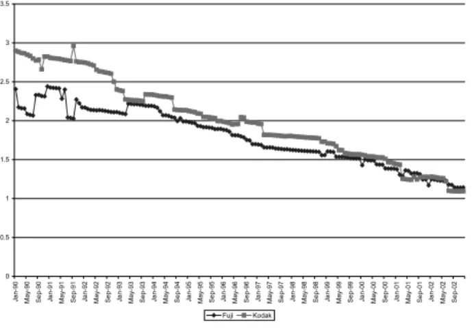
Figure 4 compares the minimum price of Kodak’s and Fuji’s film. 3 Kodak’s price has declined since around 2001. When the photo film demand began to decline in 1999, Kodak’s film price
2
The annual quanity each firm sold is calculated by annual production level and market share. The data source is explained in section 3.1.
3
Following the previous studies such as Kadiyali (1996) and Sudhir, Chintagunta, and Kadiyali (2005), the author collected the price of 24-exposure ASA200 35mm color film from various issues of Popular Photography Magazine . A problem to creating the price path of photo film is that the price of the target film varies over retail shops every month.
Then we used the minimum price among advertised shops, and consider the minimum price as the representative price of the photo film.
0 100 200 300 400 500 600 700 800
1984 1985 1986 1987 1988 1989 1990 1991 1992 1993 1994 1995 1996 1997 1998 1999 2000 2001 2002 2003 2004 2005 2006 0 2 4 6 8 10 12
Film Digital Camera
Figure 2: Numbers of 35mm film rolls and digital camera sold in the U.S. (Unit: one million)
Agfa had 0.8% and Konica had 0.3% according to Mediamark Research Inc.
Due to the demand shock by the arrival of the digital cam- era, two major film companies, Agfa and Konica, exited from the photographic film industry. AgfaPhoto, a German company producing photographic films under the name of “Agfa,” filed its insolvency on May 27, 2005. Konica announced that it would reduce the photographic film sector and put an emphasis on the digital camera sector on November 4, 2005.
Kodak and Fuji, however, announced that they would con-
tinue to produce photographic films. This implies that the pho-
tographic film industry is going to be a duopoly industry. In our
analysis, we consider this duopoly situation.
0 50 100 150 200 250 300 350 400 450 500
1985 1986 1987 1988 1989 1990 1991 1992 1993 1994 1995 1996 1997 1998 1999 2000 2001 2002
Kodak Fuji
Figure 3: Numbers of Kodak and Fuji’s 35mm film rolls sold and their trends (Unit: one million)
2.2 Comparison between Kodak and Fuji
Here we show trends in quantity sold and the price of the photo film. Figure 3 shows the time series data of quantity of Kodak and Fuji sold. 2 On the one hand, Kodak’s sales have declined since 1999 when the total 35mm film sales started to decrease. On the other hand, Fuji’s sales have increased over time from 1986.
Figure 4 compares the minimum price of Kodak’s and Fuji’s film. 3 Kodak’s price has declined since around 2001. When the photo film demand began to decline in 1999, Kodak’s film price
2
The annual quanity each firm sold is calculated by annual production level and market share. The data source is explained in section 3.1.
3
Following the previous studies such as Kadiyali (1996) and Sudhir, Chintagunta, and Kadiyali (2005), the author collected the price of 24-exposure ASA200 35mm color film from various issues of Popular Photography Magazine . A problem to creating the price path of photo film is that the price of the target film varies over retail shops every month.
Then we used the minimum price among advertised shops, and consider the
minimum price as the representative price of the photo film.
gies in the U.S. photographic film market. With the likelihood tests for model selection developed by Vuong (1989), that paper demonstrates that data is best fit to the case where Kodak and Fuji might collude in pricing and advertising after Fuji’s entry.
Sudhir et al. (2005) captures a change in competition over time in the photographic film industry. That paper finds that competitive intensity is greater in periods of high demand and lower cost, and is moderated by whether demand or costs are expected to grow or decline. That paper also finds asymmetries in the competitive responses of Kodak and Fuji. While Kodak is sensitive to demand factors, Fuji is sensitive to costs. Their results suggest that market characteristics such as observability of competitor prices can be an important determinant of how competitive intensity is affected by demand and cost conditions.
In the existing literature on declining industry, for example, Ghemawat and Nalebuff (1985, 1990) and Estive-P´erez (2005) as- sume that firms can control their capital size according to demand fluctuation. Under this assumption, both papers provide theoret- ical frameworks as to the optimal timing of exit for firms when they face declining demand. The former paper studies a duopoly model and shows a unique subgame perfect equilibrium for firms with asymmetric market shares and identical unit costs in which survivability is inversely related to size: the largest firm is the first to leave (at time 0) and the smallest firm the last. The lat- ter paper adds consumers’ quality choice problem to the model of Ghemawat and Nalebuff (1985, 1990) and demonstrates that the low-quality firm may find it optimal to stay in the market despite making temporary losses until the high quality firm concedes and exits.
To our best knowledge, no paper investigates pricing be-
0 0.5 1 1.5 2 2.5 3 3.5
Jan-90 May-90 Sep-90 Jan-91 May-91 Sep-91 Jan-92 May-92 Sep-92 Jan-93 May-93 Sep-93 Jan-94 May-94 Sep-94 Jan-95 May-95 Sep-95 Jan-96 May-96 Sep-96 Jan-97 May-97 Sep-97 Jan-98 May-98 Sep-98 Jan-99 May-99 Sep-99 Jan-00 May-00 Sep-00 Jan-01 May-01 Sep-01 Jan-02 May-02 Sep-02 Fuji Kodak
Figure 4: Price path (Unit: US dollar in the real term) lowered slightly, but it increased in 2000. Fuji’s price radically fell from the middle of 1997 to 1998. After this, the price has decreased slightly.
At the beginning of 1999 when the photo film demand started to decline, the accumulated number of the digital cam- eras sold was 2,270,000. One year later the accumulated number was 4,382,000, which is almost double of the previous year. This may be a threshold.
2.3 Literature
In this subsection we survey the literature on the photographic film industry, the digital camera industry, the firms’ behavior in declining demand, and the pricing in business cycle.
The papers by Kadiyali (1994) are the first empirical pa- pers that study strategic interaction between Kodak and Fuji.
Among them, Kadiyali (1996) examines firm-level demand-based
and cost-based explanations for entry and accommodation strate-
gies in the U.S. photographic film market. With the likelihood tests for model selection developed by Vuong (1989), that paper demonstrates that data is best fit to the case where Kodak and Fuji might collude in pricing and advertising after Fuji’s entry.
Sudhir et al. (2005) captures a change in competition over time in the photographic film industry. That paper finds that competitive intensity is greater in periods of high demand and lower cost, and is moderated by whether demand or costs are expected to grow or decline. That paper also finds asymmetries in the competitive responses of Kodak and Fuji. While Kodak is sensitive to demand factors, Fuji is sensitive to costs. Their results suggest that market characteristics such as observability of competitor prices can be an important determinant of how competitive intensity is affected by demand and cost conditions.
In the existing literature on declining industry, for example, Ghemawat and Nalebuff (1985, 1990) and Estive-P´erez (2005) as- sume that firms can control their capital size according to demand fluctuation. Under this assumption, both papers provide theoret- ical frameworks as to the optimal timing of exit for firms when they face declining demand. The former paper studies a duopoly model and shows a unique subgame perfect equilibrium for firms with asymmetric market shares and identical unit costs in which survivability is inversely related to size: the largest firm is the first to leave (at time 0) and the smallest firm the last. The lat- ter paper adds consumers’ quality choice problem to the model of Ghemawat and Nalebuff (1985, 1990) and demonstrates that the low-quality firm may find it optimal to stay in the market despite making temporary losses until the high quality firm concedes and exits.
To our best knowledge, no paper investigates pricing be-
from Survey of Current Business. Data is collected on the price of silver, which is the main input to produce photographic film, from a web site of “Kitco.” 4 This is a retailer of precious metal and its web site provides the daily per ounce price in US dollars.
Consumer Price Index is obtained from the web site of the Bureau of Labor Statistics.
Annual and monthly quantity sold of digital camera are ob- tained from three sources. One of them is Professor Juan Esteban Carranza. He provided the author the number of monthly quan- tity sold, which was collected by a leading market research firm, spanning the months between January of 1998 and September of 2001. The data has coverage of around 90% of the U.S. digital camera market. The other sources are PMA DIMA Data Digital Industry Trends Reports and CEA Market Research.
3.2 Static Duopoly Model: Price Competition
This paper estimates and shows how the demand curve for photo- graphic film changed with the introduction of the digital camera.
The paper focuses on a static duopoly model where only Kodak and Fuji (i = 1, 2) are in the market. Each firms produces only one photo film and they are differentiated.
We assume a linear demand curve as follows: for i = 1, 2 q it = a i0 + a i1 p it + a i2 p − it + a i3 I t (1) where p i is the unit price of firm i’s product and I t is the per capita income at time t. Since the market is duopoly, the rival firm’s price (p −i ) also affect the demand for product i. This specification of the demand curve is close to that in Kadiyali (1996). 5
4
Data is available at https://www.kitco.com/charts/livesilver.html
5
Kadiyali (1996) includes advertisement expenditure paid by Kodak and
havior under declining demand. However, there are papers that investigate firms’ pricing behavior under the business cycle that include periods of declining demand, i.e., recession. For example, Rotemberg and Saloner (1986) and Haltiwanger and Harrington (1991) study the possibility of price war. While the former demon- strates that price war occurs during boom, the latter finds it most difficult to collude in price during recessions. Although these pa- pers can imply the firms’ pricing behavior during recessions, i.e., when demand is declining, those models include firms’ expecta- tion that at some point of time the economy will recover for sure.
This is not what this paper focuses on: firms expect that the industry keep shrinking and may not recover.
3 Empirical Model 3.1 Data
Our empirical analysis focuses on estimation of the demand curves of Kodak and Fuji in the US market. Data are collected from various sources. These data are on firm-level prices, units sold, advertisement expenditure, and demand and cost shifters.
We collect price data from Popular Photography Magazine, a monthly magazine where mail-order firms advertise photography related products. As explained in the previous section, we collect the price of 24-exposure, ASA200 35mm color film as the represen- tative product of the market. Bi-monthly market shares of firms and industry level sales are obtained from several sources includ- ing Kadiyali (1996), Mediamark Research: Sports and Recreation Report, Wolfman Report, PMA International Trend Report and PMA Photo Industry 2006.
Quarterly per capita disposable income data is obtained
from Survey of Current Business. Data is collected on the price of silver, which is the main input to produce photographic film, from a web site of “Kitco.” 4 This is a retailer of precious metal and its web site provides the daily per ounce price in US dollars.
Consumer Price Index is obtained from the web site of the Bureau of Labor Statistics.
Annual and monthly quantity sold of digital camera are ob- tained from three sources. One of them is Professor Juan Esteban Carranza. He provided the author the number of monthly quan- tity sold, which was collected by a leading market research firm, spanning the months between January of 1998 and September of 2001. The data has coverage of around 90% of the U.S. digital camera market. The other sources are PMA DIMA Data Digital Industry Trends Reports and CEA Market Research.
3.2 Static Duopoly Model: Price Competition
This paper estimates and shows how the demand curve for photo- graphic film changed with the introduction of the digital camera.
The paper focuses on a static duopoly model where only Kodak and Fuji (i = 1, 2) are in the market. Each firms produces only one photo film and they are differentiated.
We assume a linear demand curve as follows: for i = 1, 2 q it = a i0 + a i1 p it + a i2 p − it + a i3 I t (1) where p i is the unit price of firm i’s product and I t is the per capita income at time t. Since the market is duopoly, the rival firm’s price (p −i ) also affect the demand for product i. This specification of the demand curve is close to that in Kadiyali (1996). 5
4
Data is available at https://www.kitco.com/charts/livesilver.html
5
Kadiyali (1996) includes advertisement expenditure paid by Kodak and
that we use the accumulated number of digital cameras sold D t to capture the effect of the camera instead of using monthly sales.
The paper treats the accumulated number of the digital camera sold as an exogenous variable. It, however, can be an en- dogenous variable because consumers are facing a choice between photo films and digital cameras, and in reality, photo film firms also produce digital cameras. The reason for assuming the exo- geneity is to highlight how prices respond to declining demand, and this declining demand is due to the exogenous shock under the name of technological progress. 7 Once we allow the endogeneity, the effect of price competition would be unclear because of other factors such as substitutability of photo film and digital cameras. 8 Let c(q i ) = M C i × q i be the cost for producing q i amount of good i, and M C i is firm i’s marginal cost. Marginal cost is specified to be a linear function:
M C it = c i1 Ag t + c i2 wage it + c i3 r it + c i4 oil t
where Ag is the price of silver, wage is the wage rate, r is the interest rate as a proxy of capital price, and oil is the price of crude oil. As the same with Kadiyali (1996) and Sudhir et al.
(2005), the price of silver is assumed to be common to both Kodak and Fuji. In addition, here we assume that the oil price is also common to both firms.
The firms are assumed to set their price simultaneously.
7
Different from the photo films, many manufacturers other than Kodak and Fuji produce the digital camera. Since the market of the digital camera is more competitive, Kodak or Fuji could not take strategies for photo films in order to promote the digital camera. In this point, the accumulated number of the digital camera sold is exogenous to photo film prices.
8
Ota (2011, 2019) studies a dynamic price path with a declining demand and the endogeneity of digital camera.
In order to estimate the effect of the digital camera on the demand for photo film i, we estimate the following demand curve instead of (1):
q it = a i0 + (a i1 + a i2 D t )p it + a i3 p − it + a i4 D t + a i5 I t + u it (2) where the error term u it is assumed to be normally distributed. As equation (2) shows, we include two effects of digital camera: shift and slope effects. The shift effect measures how digital camera shifts the demand curve without changes in its slope, and we capture this effect by the accumulated number of digital cameras sold D t , which is common to both firms. The slope effect measures how the slope of demand curve are changed by the digital camera.
In order to capture the slope effect, this paper puts interaction terms (D t p it ) in the demand curve. 6
The main characteristics of the digital camera is that it is a durable good as Song and Chintagunta (2003) and Carranza (2004) mention. This implies that once consumers obtain a digital camera, they will not buy a new one frequently. Thus the monthly sales of digital camera would capture the number of consumers who newly purchase a digital camera, the number does not include consumers who have already owned the camera. This is the reason
Fuji. There are two reasons this paper does not include the advertisement expenditure. First, we focus on price competition, and once we include adver- tisement expenditure it can be another strategic variable. Second, with recent data 1981-1998, Sudhir et al. (2005) shows that advertisement expenditure is not significant.
6
Another way to construct a demand curve is a derivation from a con-
sumer’s discrete choice model. Recent industrial organization studies of-
ten use this model. For example, see Bresnahan (1981), Bresnahan (1987),
Berry (1994), Berry, Levinsohn, and Pakes (1995), Nevo (2001), and Feenstra
(1995). The reason this paper does not use the model is that it would be
natural to think that consumers buy multiple numbers of photo films and
increase or decrease the number rather than to consider whether buy film or
not.
that we use the accumulated number of digital cameras sold D t to capture the effect of the camera instead of using monthly sales.
The paper treats the accumulated number of the digital camera sold as an exogenous variable. It, however, can be an en- dogenous variable because consumers are facing a choice between photo films and digital cameras, and in reality, photo film firms also produce digital cameras. The reason for assuming the exo- geneity is to highlight how prices respond to declining demand, and this declining demand is due to the exogenous shock under the name of technological progress. 7 Once we allow the endogeneity, the effect of price competition would be unclear because of other factors such as substitutability of photo film and digital cameras. 8 Let c(q i ) = M C i × q i be the cost for producing q i amount of good i, and M C i is firm i’s marginal cost. Marginal cost is specified to be a linear function:
M C it = c i1 Ag t + c i2 wage it + c i3 r it + c i4 oil t
where Ag is the price of silver, wage is the wage rate, r is the interest rate as a proxy of capital price, and oil is the price of crude oil. As the same with Kadiyali (1996) and Sudhir et al.
(2005), the price of silver is assumed to be common to both Kodak and Fuji. In addition, here we assume that the oil price is also common to both firms.
The firms are assumed to set their price simultaneously.
7
Different from the photo films, many manufacturers other than Kodak and Fuji produce the digital camera. Since the market of the digital camera is more competitive, Kodak or Fuji could not take strategies for photo films in order to promote the digital camera. In this point, the accumulated number of the digital camera sold is exogenous to photo film prices.
8
Ota (2011, 2019) studies a dynamic price path with a declining demand
and the endogeneity of digital camera.
assumes that consumers’ seasonal behavior for purchasing photo film did not change over time after 1994.
Quantity of digital camera sold: We have two data set:
one is annual data for 1996-2003 and the other is monthly data on units sold during January 1998 to September 2001 that Pro- fessor Carranza at Wisconsin-Madison provided to me. First we calculated monthly market share in each year by using Prof. Car- ranza’s data set and obtained average monthly market share. We applied the market share to the first annual data set to obtain the monthly sales of digital cameras for 1996 to 2002.
Table 1 shows summary statistics of variables after this ma- nipulation. Price and income are deflated by the Consumer Price Index, which is set to be 100 in year 1996.
Variable Obs. Mean Std. Dev. Min Max
Demand Side
Kodak quantity (no. of rolls, million) 156 34.34 8.94 20.49 49.89 Fuji quantity (no. of rolls, million) 156 8.64 3.14 3.14 15.31
Kodak price (1996 $/roll) 156 2.00 0.52 1.09 2.96
Fuji price (1996 $/roll) 156 1.79 0.36 1.14 2.44
Per-capita income (1996 $/annual) 156 19657.49 1067.17 18349.88 21728.99 Digital camera (no. of sold, thousand) 84 275.90 348.23 15.53 2263.71 Cost Side
Silver 156 4.42 0.60 3.31 6.02
US Interest rate 156 6.33 1.16 3.87 8.89
JP Interest rate 156 3.07 2.03 0.66 8.62
Oil 156 19.70 4.49 9.81 38.37
US Wage rate 156 16.36 0.39 15.71 17.86
JP Wage rate 156 18.17 6.93 8.95 41.89
Table 1: Summary Statistics: 1990-2002 (monthly otherwise noted)
The second change is that we remove seasonal effects in- cluded in photo film sales. Photographic film is mostly sold in the November-December period which is the holiday season. In order to get rid of the seasonal effect, we take a 12-month average for the quantity of photo film sold. Section 5 examines robustness by using other methods of de-trending the seasonal effects.
Then, they determines their prices so as to maximize their profit:
max pi≥ 0 π i = p i q i (p i , p −i ) − c(q i (p i , p −i )).
The first order condition for each i is q i + p i ∂q i
∂p i − ∂c
∂q i
∂q i
∂p i = 0 ⇒ p i = M C i − 1
α i1 q i . (3) As we see in the first order condition (3), price is correlated with the error term through q i . In this case, ordinary least squares doesn’t give us consistent estimates of the demand curve (2).
Then, we employ several instruments. They are components of marginal costs and pre-determined variables such as previous pe- riod’s sales of photo films and accumulated number of digital cam- eras.
3.3 Some Treatments on the Data for the Estimation For the estimation, we made two modifications to the data. The first one is about the frequency of data. The data used in this study differ in their frequency: annual, quarterly, and monthly base. The most frequent is monthly data. In order to utilize the monthly information, two variables are needed to be changed:
Quantity of films sold: This data is available on an annual
basis. Wolfman report on the photographic and imaging industry
in the United States provides bi-monthly sales share of film on
unit volume basis for 1977, 1979, 1981 and from 1984 to 1993
(13 years). We create monthly sales share by dividing the bi-
monthly share into two. However, our analysis period is from
1990 to 2002. Since we do not have such data, we calculate the
average for each monthly share using 1977-93 data and use them
as monthly sales share for 1994 to 2002. This change implicitly
assumes that consumers’ seasonal behavior for purchasing photo film did not change over time after 1994.
Quantity of digital camera sold: We have two data set:
one is annual data for 1996-2003 and the other is monthly data on units sold during January 1998 to September 2001 that Pro- fessor Carranza at Wisconsin-Madison provided to me. First we calculated monthly market share in each year by using Prof. Car- ranza’s data set and obtained average monthly market share. We applied the market share to the first annual data set to obtain the monthly sales of digital cameras for 1996 to 2002.
Table 1 shows summary statistics of variables after this ma- nipulation. Price and income are deflated by the Consumer Price Index, which is set to be 100 in year 1996.
Variable Obs. Mean Std. Dev. Min Max
Demand Side
Kodak quantity (no. of rolls, million) 156 34.34 8.94 20.49 49.89 Fuji quantity (no. of rolls, million) 156 8.64 3.14 3.14 15.31
Kodak price (1996 $/roll) 156 2.00 0.52 1.09 2.96
Fuji price (1996 $/roll) 156 1.79 0.36 1.14 2.44
Per-capita income (1996 $/annual) 156 19657.49 1067.17 18349.88 21728.99 Digital camera (no. of sold, thousand) 84 275.90 348.23 15.53 2263.71 Cost Side
Silver 156 4.42 0.60 3.31 6.02
US Interest rate 156 6.33 1.16 3.87 8.89
JP Interest rate 156 3.07 2.03 0.66 8.62
Oil 156 19.70 4.49 9.81 38.37
US Wage rate 156 16.36 0.39 15.71 17.86
JP Wage rate 156 18.17 6.93 8.95 41.89
Table 1: Summary Statistics: 1990-2002 (monthly otherwise noted)
The second change is that we remove seasonal effects in-
cluded in photo film sales. Photographic film is mostly sold in
the November-December period which is the holiday season. In
order to get rid of the seasonal effect, we take a 12-month average
for the quantity of photo film sold. Section 5 examines robustness
by using other methods of de-trending the seasonal effects.
have 6 pre-digital-camera years and 7 post-digital camera years.
Table 2 summarizes the estimation results of both Kodak and Fuji’s demand curves for three different specifications. The first column focuses on own and rival firm’s price effect on the demand, the second adds the shift effect of digital camera, and the third column is the full estimation model and it includes also the slope effect of the camera.
Kodak Fuji
(1) (2) (3) (1) (2) (3)
Own price -16.879 -14.02 -17.212 -8.244 -10.841 -11.643
(5.79)*** (5.00)*** (5.87)*** (4.84)*** (5.78)*** (5.82)***
Interaction 4.728 3.342
(3.84)*** (4.46)***
Rival price 22.204 16.592 16.015 1.446 2.623 1.64
(5.59)*** (3.95)*** (3.00)*** (1.15) (2.05)** (1.93)*
Income -0.007 -0.004
(3.33)*** (4.07)***
Digital Camera -0.108 -4.924 -0.063 -3.643
(2.02)** (3.86)*** (3.00)*** (4.48)***
Constant 27.915 32.448 166.222 20.134 22.542 97.251
(17.25)*** (11.83)*** (3.91)*** (29.57)*** (20.04)*** (4.97)***
Observations 155 155 155 155 155 155
Robust z statistics in parentheses
** significant at 5%; *** significant at 1%
Table 2: IV estimation of demand curve: 1990-2002, Twelve months moving average
First row in Table 2 shows the own price effect on the de- mand. As we can see, the estimates are statistically significant in all specification and negative, which is consistent with economic theory. The magnitude of the own price effect is stronger for Kodak’s demand than Fuji’s.
Rival firm’s price effect is shown in the third row. The esti- mates in almost all of the specifications are statistically significant and positive. This positive coefficient implies that Kodak’s film and Fuji’s film are substitutes. It is intuitive because we are com- paring the same type of film (ASA200 35mm color film) and these films are compatible to film cameras. The magnitude, however, Digital cameras are also mostly sold in the holiday season.
For this reason, for example, Gowrisankaran and Rysman (2012) adjust the sales of digital camera. This study, however, does not control the seasonal effect of digital camera sales because the de- mand curve has the accumulated number of digital camera sold, and not the monthly spot sales.
We use price data which is collected from the mail-in-order advertisement in Popular Photographic Magazine. One concern about the price may be that it is retail price, not the wholesale price. It would be better to use the wholesale price because our model captures producers’ pricing behavior but that price data is unavailable.
4 Estimation
4.1 Endogeneity of Price
Since firms compete in price, the demand curve (1) has four en- dogenous variables: p it , p − it , D t p it , and D t p − it . The OLS regres- sion returns inconsistent estimates when there are endogenous variables on the right hand side. To avoid this problem, we em- ploy instrumental variables and estimate the demand curve with the generalized method of moments (GMM). In the following es- timation, this paper uses, as the instruments, four cost factors (silver price, wage, interest rate as a proxy of capital price, and oil price) and two pre-determined variables (previous period’s sales of Kodak and Fuji).
4.2 Estimation Results
We estimate the demand curve using data from 1990-2002. In our
data set, the digital camera was introduced in 1996, so we then
have 6 pre-digital-camera years and 7 post-digital camera years.
Table 2 summarizes the estimation results of both Kodak and Fuji’s demand curves for three different specifications. The first column focuses on own and rival firm’s price effect on the demand, the second adds the shift effect of digital camera, and the third column is the full estimation model and it includes also the slope effect of the camera.
Kodak Fuji
(1) (2) (3) (1) (2) (3)
Own price -16.879 -14.02 -17.212 -8.244 -10.841 -11.643
(5.79)*** (5.00)*** (5.87)*** (4.84)*** (5.78)*** (5.82)***
Interaction 4.728 3.342
(3.84)*** (4.46)***
Rival price 22.204 16.592 16.015 1.446 2.623 1.64
(5.59)*** (3.95)*** (3.00)*** (1.15) (2.05)** (1.93)*
Income -0.007 -0.004
(3.33)*** (4.07)***
Digital Camera -0.108 -4.924 -0.063 -3.643
(2.02)** (3.86)*** (3.00)*** (4.48)***
Constant 27.915 32.448 166.222 20.134 22.542 97.251
(17.25)*** (11.83)*** (3.91)*** (29.57)*** (20.04)*** (4.97)***
Observations 155 155 155 155 155 155
Robust z statistics in parentheses
** significant at 5%; *** significant at 1%
Table 2: IV estimation of demand curve: 1990-2002, Twelve months moving average
First row in Table 2 shows the own price effect on the de- mand. As we can see, the estimates are statistically significant in all specification and negative, which is consistent with economic theory. The magnitude of the own price effect is stronger for Kodak’s demand than Fuji’s.
Rival firm’s price effect is shown in the third row. The esti-
mates in almost all of the specifications are statistically significant
and positive. This positive coefficient implies that Kodak’s film
and Fuji’s film are substitutes. It is intuitive because we are com-
paring the same type of film (ASA200 35mm color film) and these
films are compatible to film cameras. The magnitude, however,
responds to own price and rival firm’s price more than Fuji’s de- mand does. Second, the introduction of the digital camera shifts both demand curves of photo films downward, and causes the demand curves to be more inelastic to own price.
Heterogeneity in consumers’ price sensitivity to the photo- graphic film could explain these findings. Our hypothesis is as fol- lows. Consumers have their own preference to photographic film and this preference is related with their price sensitivity. Further assume that consumers are different only in their price sensitiv- ity. Our hypothesis is that consumers who buy Kodak are more diverse than those who buy Fuji and that much of Fuji’s customer base is price sensitive.
In order to understand the estimation results, we need to consider the size of sales of the firms. As Figure 3 demonstrates, there is a big gap between Kodak’s sales in volume and Fuji’s. In 2002, Kodak’s sales is about four times that Fuji’s sales and the difference was larger before 2002. Taking this size difference into account, we can rethink the observations. If consumers of Kodak and Fuji are distributed similarly in terms of price sensitivity, the effect of own and rival price on Kodak’s demand is about four times larger than that for Fuji. The estimates in Table 2, however, shows that the own price effect of Kodak’s demand is less than twice of Fuji’s own effect. From this point of view, we reinterpret the estimation results as follows: (1) While the own price effect is bigger for Fuji, the rival price effect is bigger for Kodak; (2) Both the shift and slope effects of digital camera are bigger for Fuji’s demand.
Our hypothesis to explain the results is then that consumers who buy Kodak are more diverse than Fuji’s and much of Fuji’s base is price sensitive. On the one hand, since there are more are different between them. Similar to the own price effect, the
rival firm’s price effect is also stronger for Kodak’s demand.
Here we look at the effects of the digital camera on the photo film demand. The shift and slope effects of the camera are shown in the fifth and second row, respectively. As we expect, the shift effect shows a negative relationships with both photo film demands. That is, ceteris paribus, the digital camera makes the photo film demand shift downward. This effect also is stronger for Kodak but the difference is not big.
The slope effects of digital camera captures how the slope of the demand curve changes. The effect is shown in the third row of the table, and it is statistically significant and positive to both photo film demand. This means that the digital camera makes both Kodak and Fuji’s demand curves steeper, i.e., more price- inelastic. The magnitude is slightly stronger for Kodak’s demand.
Overall, the introduction of the digital camera affects both Kodak and Fuji’s film in the same direction, and its magnitude does not change much between the firms.
Finally, we see the effects of income as a demand shifters.
The fourth row in Table 2 shows the effects of income on the photo film demand. Income has a negative effect on both demands. It is not consistent with economic theory but it is consistent with a previous study: Sudhir et al. (2005) report that income is nega- tive and significant for Kodak’s demand and it is not significant for Fuji.
4.3 Interpretation: Consumers’ Price Sensitivity and a Cream Skimming Story
In this subsection, we seek an underling theory to explain the ob-
servations. Our two main findings are: First, Kodak’s demand
responds to own price and rival firm’s price more than Fuji’s de- mand does. Second, the introduction of the digital camera shifts both demand curves of photo films downward, and causes the demand curves to be more inelastic to own price.
Heterogeneity in consumers’ price sensitivity to the photo- graphic film could explain these findings. Our hypothesis is as fol- lows. Consumers have their own preference to photographic film and this preference is related with their price sensitivity. Further assume that consumers are different only in their price sensitiv- ity. Our hypothesis is that consumers who buy Kodak are more diverse than those who buy Fuji and that much of Fuji’s customer base is price sensitive.
In order to understand the estimation results, we need to consider the size of sales of the firms. As Figure 3 demonstrates, there is a big gap between Kodak’s sales in volume and Fuji’s. In 2002, Kodak’s sales is about four times that Fuji’s sales and the difference was larger before 2002. Taking this size difference into account, we can rethink the observations. If consumers of Kodak and Fuji are distributed similarly in terms of price sensitivity, the effect of own and rival price on Kodak’s demand is about four times larger than that for Fuji. The estimates in Table 2, however, shows that the own price effect of Kodak’s demand is less than twice of Fuji’s own effect. From this point of view, we reinterpret the estimation results as follows: (1) While the own price effect is bigger for Fuji, the rival price effect is bigger for Kodak; (2) Both the shift and slope effects of digital camera are bigger for Fuji’s demand.
Our hypothesis to explain the results is then that consumers
who buy Kodak are more diverse than Fuji’s and much of Fuji’s
base is price sensitive. On the one hand, since there are more
Price elasticity Data Obs Mean SD Min Max
Kodak 1990-2002 156 -1.04 0.35 -2.44 -0.57
1990-1995 72 -1.32 0.32 -2.44 -0.99
1996-2002 84 -0.80 0.14 -1.01 -0.57
Fuji 1990-2002 156 -2.75 1.14 -4.95 -1.17
1990-1995 72 -3.87 0.51 -4.95 -2.89
1996-2002 84 -1.79 0.45 -2.83 -1.17
Table 3: Own price elasticity of demand without the slope effect:
The case of specification (3)
mate own price elasticity of the demand as follows:
ϵ t = ∂q t /q t
∂p t /p t = (a 1 + a 2 D t ) ( p t
q t )
⇒ ˆ ϵ t = (ˆ a 1 + ˆ a 2 D t ) ( p t
q t )
. In our data set, the digital camera was introduced in 1996. In order to see how the own price elasticity changes, we report it for three different time periods: 1990-2002 (whole period), 1990-1995 (pre digital camera period) and 1996-2002 (post digital camera period).
To focus on the shift effect of the digital camera on the changes in the price elasticity of demand, first, we show the own price elasticity without the slope effect. This elasticity is esti- mated by ˆ ϵ t = ˆ a 1 (p t /q t ) and Table 3 shows the own price elas- ticity for each time period based on the estimates of specification (3). For both firms’ demand curve, we see that the own price elasticity becomes smaller in absolute value in the post-digital camera period, which means that the demand curves get price inelastic. This implies that consumers who are sensitive to the price of photo films switch to the digital camera.
Table 4 shows the own price elasticity of demand with the slope effect. As we can see from the table, the trend of the change in the elasticity is the same with the above: the demand curves become more price inelastic after the introduction of digital cam- price-sensitive consumers in Fuji’s customer, Fuji’s demand is af-
fected by its pricing. That’s why Fuji’s own price effect is stronger than Kodak’s own price effect. On the other hand, more of Fuji’s consumers will switch to Kodak if Fuji’s price increases because again Fuji’s consumers are more price sensitive. This explains that the rival price effect is bigger for Kodak.
We might ask: how can we justify the hypothesis? There are two ways to answer. First, as Figure 4 shows, Fuji’s price has been lower than Kodak’s until the very end of our sample period. Since in general it is difficult to distinguish any technical difference between Kodak and Fuji’s films, the lower price should be attractive to price sensitive consumers. Second, Kodak is the dominant photo film company in the U.S., and Fuji is a minor firm.
This generates a strength in Kodak’s brand, and the strength would make consumers who are relatively price insensitive buy Kodak’ film.
Then what type of consumers does the digital camera take away from the photo film market? The estimation results show that both Kodak and Fuji’s demand curve become more price inelastic after the introduction of the digital camera. This is con- sistent with a “cream-skimming” story that the digital camera takes away the more price-sensitive customers, leaving the price- insensitive customers. Remember that after reconsidering the dif- ference in sales size, the shift and slope effects of digital camera is larger for Fuji’s demand where much of its consumer base is price sensitive.
The changes in price elasticity of demand also support the
cream-skimming story and the consumers’ price sensitivity hy-
pothesis. From the demand curve (2), we can calculate and esti-
Price elasticity Data Obs Mean SD Min Max
Kodak 1990-2002 156 -1.04 0.35 -2.44 -0.57
1990-1995 72 -1.32 0.32 -2.44 -0.99
1996-2002 84 -0.80 0.14 -1.01 -0.57
Fuji 1990-2002 156 -2.75 1.14 -4.95 -1.17
1990-1995 72 -3.87 0.51 -4.95 -2.89
1996-2002 84 -1.79 0.45 -2.83 -1.17
Table 3: Own price elasticity of demand without the slope effect:
The case of specification (3)
mate own price elasticity of the demand as follows:
ϵ t = ∂q t /q t
∂p t /p t = (a 1 + a 2 D t ) ( p t
q t )
⇒ ˆ ϵ t = (ˆ a 1 + ˆ a 2 D t ) ( p t
q t )
. In our data set, the digital camera was introduced in 1996. In order to see how the own price elasticity changes, we report it for three different time periods: 1990-2002 (whole period), 1990-1995 (pre digital camera period) and 1996-2002 (post digital camera period).
To focus on the shift effect of the digital camera on the changes in the price elasticity of demand, first, we show the own price elasticity without the slope effect. This elasticity is esti- mated by ˆ ϵ t = ˆ a 1 (p t /q t ) and Table 3 shows the own price elas- ticity for each time period based on the estimates of specification (3). For both firms’ demand curve, we see that the own price elasticity becomes smaller in absolute value in the post-digital camera period, which means that the demand curves get price inelastic. This implies that consumers who are sensitive to the price of photo films switch to the digital camera.
Table 4 shows the own price elasticity of demand with the
slope effect. As we can see from the table, the trend of the change
in the elasticity is the same with the above: the demand curves
become more price inelastic after the introduction of digital cam-
In order to remove the seasonal effect of photo film sales, we take a twelve-month moving average on quantity sold in the esti- mation of equation (2). As a robustness check, we use a monthly dummy instead of the moving average.
Results are in Table 6 where the estimates of monthly dum- mies are omitted. All but the rival price effect for Fuji’s demand and income have expected sign and statistically significant es- timates. The insignificance of Fuji’s rival price effect, however, would support the interpretation shown before: while the own price effect is bigger for Fuji, the rival price effect is bigger for Kodak. It is because the own price effect is bigger for Fuji after considering the difference in sales size, and Fuji’s demand does not respond to rival firm’s price. The insignificance of income effect would be due to the monthly dummy variable. Since the income effect is negative in the previous estimation, this insignif- icance would come from the monthly dummy variable that can well capture the variation of the number of photo film sold. The both shift and slope effects of digital camera is consistent with the previous estimates.
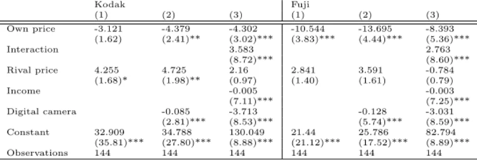
The second robustness check is to use another data span.
Instead of using data from 1990, here we use 1991-2002 that con- tains 5 pre-digital camera periods (1991-1995) and 7 post-digital camera periods (1996-2002). Since the new sample period have heavier weight on the post-digital camera, the effects of digital camera would reflect on estimation results more strongly. If we have the same results with the previous ones, our results especially on the effects of digital camera are more robust over time.
Table 7 shows the estimation results with the sample pe- riod, 1991-2002, with a twelve-month moving average on quantity sold. All but the rival price effect for Fuji’s demand of the result
Price elasticity Data Obs Mean SD Min Max
Kodak 1990-2002 156 -0.47 1.16 -2.44 3.10
1990-1995 72 -1.32 0.32 -2.44 -0.99
1996-2002 84 0.25 1.14 -0.98 3.10
Fuji 1990-2002 156 -1.51 2.88 -4.95 6.60
1990-1995 72 -3.87 0.51 -4.95 -2.89
1996-2002 84 0.50 2.51 -2.82 6.60
Table 4: Own price elasticity of demand: The case of specification (3)
Source Firms Data Mean Notes
Kadiyali (1996) Kodak 1970-1979 -0.64
1980-1990 -0.20
Fuji 1980-1990 -0.03
Sudhir et. al (2005) Kodak 1981-1998 -0.40 *
Fuji 1981-1998 -0.30 **
* author’s calculation when Kodak’s share is 70%.
** author’s calculation when Fuji’s share is 20%.
Table 5: Own price elasticity of demand: Previous studies era. The slope effect of digital camera makes the demand curves more price inelastic.
Table 5 shows own price elasticity estimated by previous studies (Kadiyali, 1996; Sudhir et al., 2005), which do not con- sider the introduction of the digital camera. These numbers con- trast the big effect of the digital camera on the demand for photo films.
5 Robustness of the Estimation Results
In this section, we check the robustness of the estimation re-
sults. We demonstrate the robustness by considering: (1) an-
other method for de-trending seasonal effects of photo film sales,
(2) changing the sample periods, and (3) using other specifica-
tions of the demand curve. Overall, we see that the estimation
results are robust.
In order to remove the seasonal effect of photo film sales, we take a twelve-month moving average on quantity sold in the esti- mation of equation (2). As a robustness check, we use a monthly dummy instead of the moving average.
Results are in Table 6 where the estimates of monthly dum- mies are omitted. All but the rival price effect for Fuji’s demand and income have expected sign and statistically significant es- timates. The insignificance of Fuji’s rival price effect, however, would support the interpretation shown before: while the own price effect is bigger for Fuji, the rival price effect is bigger for Kodak. It is because the own price effect is bigger for Fuji after considering the difference in sales size, and Fuji’s demand does not respond to rival firm’s price. The insignificance of income effect would be due to the monthly dummy variable. Since the income effect is negative in the previous estimation, this insignif- icance would come from the monthly dummy variable that can well capture the variation of the number of photo film sold. The both shift and slope effects of digital camera is consistent with the previous estimates.
The second robustness check is to use another data span.
Instead of using data from 1990, here we use 1991-2002 that con- tains 5 pre-digital camera periods (1991-1995) and 7 post-digital camera periods (1996-2002). Since the new sample period have heavier weight on the post-digital camera, the effects of digital camera would reflect on estimation results more strongly. If we have the same results with the previous ones, our results especially on the effects of digital camera are more robust over time.
Table 7 shows the estimation results with the sample pe-
riod, 1991-2002, with a twelve-month moving average on quantity
sold. All but the rival price effect for Fuji’s demand of the result
Kodak Fuji
(1) (2) (3) (1) (2) (3)
Own price -3.121 -4.379 -4.302 -10.544 -13.695 -8.393
(1.62) (2.41)** (3.02)*** (3.83)*** (4.44)*** (5.36)***
Interaction 3.583 2.763
(8.72)*** (8.60)***
Rival price 4.255 4.725 2.16 2.841 3.591 -0.784
(1.68)* (1.98)** (0.97) (1.40) (1.61) (0.79)
Income -0.005 -0.003
(7.11)*** (7.25)***
Digital camera -0.085 -3.713 -0.128 -3.031
(2.81)*** (8.53)*** (5.74)*** (8.59)***
Constant 32.909 34.788 130.049 21.44 25.786 82.794
(35.81)*** (27.80)*** (8.88)*** (21.12)*** (17.52)*** (8.89)***
Observations 144 144 144 144 144 144
Robust z statistics in parentheses
* significant at 10%; ** significant at 5%; *** significant at 1%
Table 7: IV estimation of demand curve: 1991-2002, Twelve month moving average
sults are summarized in Table 8. Most estimates are consistent with the previous results. The only exception is the interaction term (the slope effect of the digital camera) for Kodak’s demand curve. Kodak’s demand does not become more price inelastic.
This observation, however, does not deny our interpretation, a cream-skimming story, such that the digital camera affect price sensitive consumers who are distributed more in Fuji’s customer base rather than Kodak’s base. As Table 8 shows, the slope ef- fect on Fuji’s demand is statistically significant and makes Fuji’s demand more price inelastic.
Previous studies of the U.S. photographic film industry (Kadiyali, 1996; Sudhir et al., 2005) included advertisement ex- penditure in the demand curve. This study removes the adver- tisement expenditure because as we see below we get a negative coefficient on the expenditure where it should be positive. How- ever this result is not inconsistent with previous studies. With 1980-1998 data, Sudhir et al. (2005) demonstrates that the ef- fect of the expenditure is insignificant, while with 1970-1990 data
Kodak Fuji
(1) (2) (3) (1) (2) (3)
Own price -10.391 -9.687 -7.279 -6.925 -7.626 -8.233
(7.94)*** (7.76)*** (6.82)*** (6.57)*** (6.66)*** (4.83)***
Interaction 1.872 1.34
(2.57)** (2.36)**
Rival price 14.283 12.124 11.249 0.689 0.709 1.076
(7.90)*** (6.26)*** (4.00)*** (0.87) (0.89) (1.36)
Income -0.001 -0.001
(0.57) (1.41)
Digital camera -0.098 -2.102 -0.049 -1.498
(2.75)*** (2.90)*** (1.94)* (2.43)**
Constant 38.167 41.397 52.594 21.625 23.053 44.088
(28.84)*** (21.60)*** (1.82)* (32.39)*** (21.66)*** (2.64)***
Observations 155 155 155 155 155 155
Robust z statistics in parentheses
** significant at 5%; *** significant at 1%
Table 6: IV estimation of demand curve: 1990-2002, Monthly dummy (Estimates are omitted)
are consistent with the previous results shown in Table 2. More importantly, we can check the consistent results of both shift and slope effects of digital camera by using different sample periods’
data.
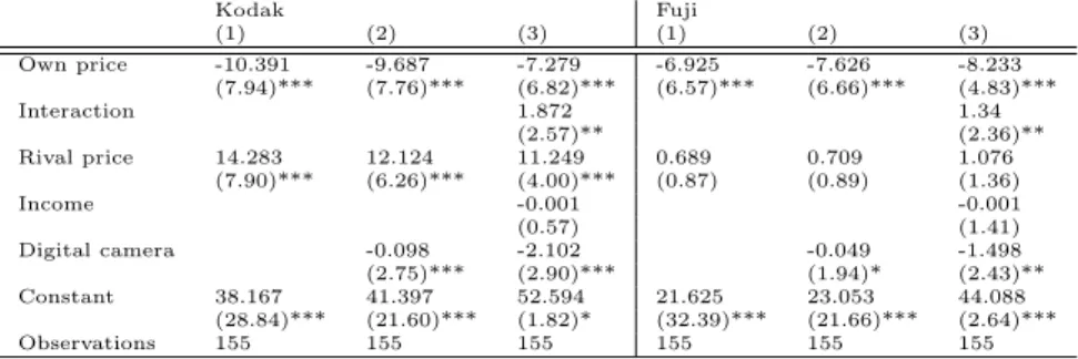
The final way to check robustness is by using different spec- ifications of the demand curve. Here we show two modifications on the demand curve. First, we use a different form of the slope effect of the digital camera. Second, we add a new variable, adver- tisement expenditure, which is used in the previous studies such as Kadiyali (1996) and Sudhir et al. (2005).
Our sample periods (1990-2002) capture the introductory stage of the digital camera since it was introduced in 1996. Thus it is possible to think that even if consumers buy a digital camera, they still buy photo films because the quality of digital camera was not sufficient. This concern would be avoided by adding a factor that weakens the effect of the digital camera.
For this purpose, we use another interaction term √
D t p it
instead of D t p it in the demand curve (2). The estimation re-
Kodak Fuji
(1) (2) (3) (1) (2) (3)
Own price -3.121 -4.379 -4.302 -10.544 -13.695 -8.393
(1.62) (2.41)** (3.02)*** (3.83)*** (4.44)*** (5.36)***
Interaction 3.583 2.763
(8.72)*** (8.60)***
Rival price 4.255 4.725 2.16 2.841 3.591 -0.784
(1.68)* (1.98)** (0.97) (1.40) (1.61) (0.79)
Income -0.005 -0.003
(7.11)*** (7.25)***
Digital camera -0.085 -3.713 -0.128 -3.031
(2.81)*** (8.53)*** (5.74)*** (8.59)***
Constant 32.909 34.788 130.049 21.44 25.786 82.794
(35.81)*** (27.80)*** (8.88)*** (21.12)*** (17.52)*** (8.89)***
Observations 144 144 144 144 144 144
Robust z statistics in parentheses
* significant at 10%; ** significant at 5%; *** significant at 1%