curves, and tropical ideals

Tropical polynomials being the minimum finishing time of project networks, genera of tropicalizations of

curves, and tropical ideals

2018

Takaaki Ito

Department of Mathematics and Information Sciences

Tokyo Metropolitan University

Contents

1 Introduction 3

1.1 Preliminary . . . . 4 1.2 Outline of thesis . . . . 5 2 A characterization for tropical polynomials being the

minimum finishing time of project networks 9 2.1 Project networks . . . . 9 2.2 Term extendability . . . . 10 2.3 Term graphs . . . . 14 3 Genera of the tropicalizations of curves over an alge-

braic function fields of one variable 20 3.1 Preliminary . . . . 20 3.1.1 Tropical geometry . . . . 20 3.1.2 Algebraic function field of one variable . . . . 22 3.1.3 The Hessian form of an elliptic curve . . . . . 23 3.2 Proof of the main theorem . . . . 23 4 Tropical ideals in tropical polynomial function semir-

ings 25

4.1 Tropical polynomial function semirings . . . . 25 4.2 One variable tropical polynomial function semiring . 29 4.3 Tropical ideals in one variable tropical polynomial

function semiring . . . . 38 4.4 Unexpected examples of tropical ideals in tropical

polynomial semirings . . . . 52

1 Introduction

Tropical geometry is developing with several branches of mathemat- ics, geometry, algebra, and applied mathematics.

Most studies are based on geometric motivations. For exam- ple, the computation of Gromov-Witten invariants is well taken up.

Mikhalkin showed that the Gromov-Witten invariants of projective plane can be computed by counting tropical curves in [17]. This result made tropical geometry known as a useful combinatorial tool for problems in algebraic geometry. The second example is the the- ory of tropicalizations. The term“tropicalization” is a general term for the processes of associating a tropical variety to an algebraic variety, or for the resulting tropical variety itself. Gathmann intro- duces several ways of tropicalization in [5]. In most papers which treats tropicalizations, the coefficient field K is required to be alge- braically closed. The tropicalizations of varieties over an arbitrary field are studied by Gubler in [7]. The third example is tropical in- tersection theory. Based on Mikhalkin’s ideas in [18], which is called stable intersections, Allermann and Rau established the foundation in [1]. Katz shows in [10] that the theory in [1] is equivalent to the fan displacement rule of [3]. Jensen and Yu give another definition of stable intersections in [11], which is preferable for computations to Allermann and Rau’s definition and fan displacement rule. In [16], Meyer extended the stable intersections in R

to tropical toric varieties.

Recently, an algebraic foundation for tropical geometry is tried to develop. Giansiracusa and Giansiracusa define tropical schemes in [4], which are congruences on the semiring of tropical polyno- mials. Maclagan and Rinc´ on found a relationship among tropical schemes, ideals in the semiring of tropical polynomials, and valu- ated matroids in [13]. Based on this relationship, the authors of [13]

defined tropical ideals in [14], which generalize the tropicalizations of classical ideals. Viro suggests another approach in [20], which uses hyperfields.

Tropical geometry has applications to the other fields of math- ematics. For instance, Kobayashi and Odagiri illustrated the adja- cency of paths in project networks by using tropical varieties in [12].

Speyer and Strumfels showed that the space of phylogenetic trees

coincides with the tropical Grassmannian of 2-planes.

This thesis consists of three studies, which are based on geomet- ric, algebraic, and applied mathematical interest, respectively. The author believe that this work helps the development of comprehen- sive study in tropical geometry.

1.1 Preliminary

We now recall the basic definitions and facts in tropical geometry.

For details of this section, see [15].

In this thesis, a valuation on a field K means a non-archimedean additive valuation on K, namely, a map v : K → R ∪{∞} such that

• v(a) = ∞ if and only if a = 0,

• v(ab) = v(a) + v(b),

• v(a + b) ≥ min { v(a), v(b) } .

The trivial valuation is the following map:

a 7→

{

0 if a ̸ = 0

∞ if a = 0.

Let K be an algebraically closed field with a nontrivial valuation v.

Consider the map

Val : G

→ R

, (a

, . . . , a

) 7→ ( − v(a

), . . . , − v(a

)).

Here we use − v(a

) but not v(a

), because the author adopts the max-plus convention. Let X be a subvariety of a torus G

. We define the tropicalization trop(X) of X as the closure of Val(X) ⊂ R

via the Euclidean topology. trop(X) is the support of a polyhedral complex in R

.

There is another definition of tropicalizations, which uses trop- ical polynomials. The tropical semifield is the semifield T = ( R ∪ {−∞} , ⊕ , ⊙ ), where the addition is a ⊕ b := max { a, b } and the mul- tiplication is a ⊙ b := a + b. In this paper, we usually omit the symbol ⊙ . A tropical polynomial of x

, . . . , x

is a formal sum of the form

a

x

⊕ a

x

⊕ · · · ⊕ a

x

for some a

∈ T and u

∈ Z

, where x

= x

· · · x

if u =

(u

, . . . , u

). The set T [x

, . . . , x

] of all tropical polynomials of

x

, . . . , x

forms a semiring via the natural addition and multiplica- tion. We call T [x

, . . . , x

] the tropical polynomial semiring. Also we define the tropical Laurent polynomial semiring T [x

, . . . , x

] as usual sense.

Each nonzero tropical Laurent polynomial defines a piecewise linear map from R

to R . For a nonzero tropical Laurent polynomial f ∈ T [x

, . . . , x

], we define the tropical variety V (f ) as

V (f ) = { w ∈ R

| f is not differentiable at w ∈ R

} . For a Laurent polynomial f = ∑

u

a

x

∈ K [x

, . . . , x

], we de- fine its tropicalization as trop

(f ) := ⊕

u

( − v(a

)) ⊙ x

, which is a tropical Laurent polynomial. Then the tropical variety V (trop(f )) coincides with the tropicalization trop(V (f )) (Kapranov’s theorem [2]). For a subvariety X of a torus G

defined by the ideal I ⊂ K[x

, . . . , x

], we have the following equality:

trop(X) = ∩

f∈I

V (trop(f )).

1.2 Outline of thesis

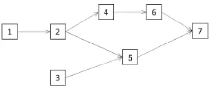
In Section 2 we study a characterization for tropical polynomials be- ing the minimum finishing time of project networks. A project net- work consists of some activities, where each activity can be started after all the preceding activities have finished. We may regard the set of activities as an ordered set. By taking the Hasse diagram, a project network is represented as a directed acyclic graph. Each activity is endowed with a non-negative real number t

, called time cost. We may consider that the time cost of an activity represents the time to complete the activity. The minimum finishing time of a project network is the minimum time taken for finishing all the ac- tivities in that network. The minimum finishing time is represented by a tropical polynomial of t

, . . . , t

.

A tropical polynomial is called a realizable polynomial or an R-

polynomial if it can be realized as the minimum finishing time of

a project network. An R-polynomial satisfies the following three

conditions (Proposition 2 in [12]): (1) the degree on each variable is

exactly one, (2) the coefficient of each term is a unity and (3) no term

is divisible by any other terms (‘indivisibility’). A tropical polyno-

mial satisfying those conditions is called prerealizable polynomial or

Ϯ ϰ

㻡 ϲ

ϳ ϭ

ϯ

Figure 1: project network

P -polynomial. A P -polynomial is not always an R-polynomial. A simplest example of a P -polynomial which is not an R-polynomial is t

t

⊕ t

t

⊕ t

t

([12]).

A characterization of R-polynomials using poset is known (Propo- sition 2.1.3), but it is not effective for judging whether a given P - polynomial is an R-polynomial. In this paper, we introduce another characterization by graph theory. We do this by two steps. We first show that every R-polynomial satisfies a term extendability condi- tion, which we will define later, and prove the following theorem.

Theorem 1.2.1. There is a one-to-one correspondence between the set of P -polynomials f (t) = f (t

, . . . , t

) having term extendability and the set of simple graphs with the vertex set [n]. Via this cor- respondence, two simple graphs are isomorphic if and only if the corresponding P -polynomials coincide up to a permutation of vari- ables.

Secondly, by this theorem, we will give a characterization for R- polynomials in the context of graph theory. The following is our main theorem.

Theorem 1.2.2. Let f(t) be a P -polynomial of degree d with the term extendability. Then f(t) is an R-polynomial if and only if there is a vertex coloring of the term graph T G(f) with the color set { 1, . . . , d } such that every increasing path of three vertices is a clique of T G(f ).

By this theorem, we can give some examples of judging whether a given polynomial is an R-polynomial.

As for P -polynomials, we have a correspondence between the set of P -polynomials and the set of abstract complexes.

In Section 3, we discuss genera of the tropicalizations of curves

over an algebraic function fields of one variable. The genus of the

tropicalization of a subvariety of G

is not always equal to that of original subvariety (see Example 3.1.6). In this section, we consider the tropicalizations of curves over an algebraic function field over C of one variable. By varying a valuation on the coefficient field, we give a tropicalization which keeps the genus.

The main theorem of this section is the following.

Theorem 1.2.3. Let E be an elliptic curve over an algebraic func- tion field K of one variable on C . Suppose that the j–invariant of E is not in C . Then there exist

• a finite extension L of K,

• an elliptic curve C ⊂ P

over L birationally equivalent to the scalar extension E ×

SpecL,

• a valuation v on L

such that the tropicalization of C ∩ T via v has genus one, where T is a big torus of P

.

In Section 4 we study tropical ideals in tropical polynomial func- tion semirings. In [14], Maclagan and Rinc´ on defined the tropical variety V (I) associated to an ideal I ⊂ T [x

, . . . , x

] as

V (I) = ∩

f∈I

V (f).

A tropical variety is expected to be the support of a finite polyhedral complex. However, a counterexample is given in [14]. To avoid this problem, in [14], the authors define tropical ideals as follows.

Definition 1.2.4. An ideal I in T [x

, . . . , x

] is a tropical ideal if, for any f, g ∈ I and any monomial x

for which [f ]

= [g]

̸ = −∞ , there exists h ∈ I such that [h]

= −∞ and [h]

≤ [f ]

⊕ [g]

for all v, with the equality holding whenever [f]

̸ = [g]

.

Here we use the notation [f ]

to denote the coefficient of the mono- mial x

in f.

They show that for any tropical ideal I, the set V (I) is the sup-

port of a finite polyhedral complex. Moreover, they proved that

tropical ideals satisfy the ascending chain condition and also that

tropical Nullstellensatz holds, which are not true for arbitrary ideals.

In this section, we consider a “function version” of tropical ideals.

We define tropical ideals in the tropical polynomial function semir- ings T [x

, . . . , x

]/ ∼ , where the relation ∼ is defined as f ∼ g if and only if f(a) = g(a) for any a ∈ R

. The definition of our tropical ideals is analogous to [14]. One of the advantages of considering in T [x

, . . . , x

]/ ∼ instead of T [x

, . . . , x

] is that we can always fac- torize a tropical polynomial function of one variable into a product of tropical polynomial functions of degree one (see Lemma 4.2.1 or [6]).

As a first step of the study of our tropical ideals, we focus on the case of one variable. The followings are our main theorems.

Theorem 1.2.5. For any tropical polynomial function φ ∈ T [x]/ ∼ , the set φ ⊙ ( T [x]/ ∼ ) := { φ ⊙ ψ | ψ ∈ T [x]/ ∼} is a tropical ideal in T [x]/ ∼ .

Theorem 1.2.6. Every tropical ideal in T [x]/ ∼ is of the form φ ⊙ ( T [x]/ ∼ ) for some φ ∈ T [x]/ ∼ .

These theorems say that T [x]/ ∼ is like a PID. As a consequence of the theorems, it follows that our tropical ideals are closed under the intersection, and that we can add, multiply and generate trop- ical ideals. In fact, these properties do not hold for Maclagan and Rinc´ on’s tropical ideals.

Acknowledgment. I would like to express my sincere gratitude

to Professor Masanori Kobayashi for advice concerning this thesis. I

also thank Professor Yukihiro Uchida, Professor Chikara Nakayama,

Professor Kaori Suzuki and Doctor Kouhei Sato for useful comments

and discussions.

2 A characterization for tropical polynomials be- ing the minimum finishing time of project net- works

2.1 Project networks

In this section, we recall the relation between project networks and tropical algebra. For detail of this section, see [12].

Formally, a project network is an acyclic directed graph with no short-cuts, where a graph is said with no short-cuts if the following condition holds: if there are two distinct paths from activity a to activity b, then both paths consist of more than one arrow.

Proposition 2.1.1 ([12, Proposition 1]). Let X be a finite set.

There is a one-to-one correspondence between the set of partial or- ders on X and the set of simple directed graphs with vertex set X without cycles or short-cuts.

The correspondence in Proposition 2.1.1 is given as follows. For a given partial order of X, we take its Hasse diagram as the cor- responding graph. For a given project network with the vertex set X, we define the corresponding partial order on X so that, for each arrow, its head is greater than its tail.

Each activity is endowed with a non-negative real number t

, called time cost. We may consider that the time cost of an activity represents the time to complete the activity. The minimum finishing time of a project network is the minimum time taken for finishing all the activities in that network. Then the minimum finishing time is a function of t

, . . . , t

, which has following properties.

Proposition 2.1.2 ([12, Proposition 2]). The minimum finishing time f (t) = f (t

, . . . , t

) can be written as a tropical polynomial of t

, . . . , t

satisfying the following three conditions:

(1) the degree on each variable is exactly one, (2) the coefficient of each term is a unity,

(3) no term is divisible by any other terms. (‘indivisibility’)

A tropical polynomial is called a realizable polynomial or an R-

polynomial if it can be obtained as the minimum finishing time of a

project network. Also, a tropical polynomial is called a prerealizable

polynomial or a P -polynomial if it satisfies the condition (1) − (3).

A P -polynomial is not always an R-polynomial.

For a set of variables { t

}

and a subset I ⊂ Λ, we denote the monomial ∏

i∈I

t

by t

. We know the following characterization of R-polynomials.

Proposition 2.1.3 ([12, Proposition 3]). Let f (t) = ⊕

I∈I

t

be a tropical polynomial in n variables. Then f (t) is an R-polynomial if and only if there exist a poset structure on the index set [n] such that

I is a maximal totally ordered subset ⇔ t

is a term of f(t).

If we want to check whether a given P -polynomial is an R- polynomial by this characterization, for example, we may list up the all poset structure on [n]. However, the calculation amount is not realistic. Thus we introduce another approach in the later section.

2.2 Term extendability

In this section, we introduce our key condition, called term ex- tendability, which holds for every R-polynomial. For a given P - polynomial, checking for term extendability is easier than checking whether the polynomial is an R-polynomial. Many P -polynomials are excluded from the candidates for R-polynomials by restricting via this condition. Furthermore, in the next section, we will con- struct a correspondence between P -polynomials with term extend- ability and simple graphs. The correspondence is important for our new characterization. Unfortunately, there is a P -polynomial that has term extendability but is not an R-polynomial. We will see some examples of such polynomials in this section.

In the later of this section, we will estimate the number of terms of R-polynomials by using term extendability condition. In addition, we will show that if the number of terms is smaller than 5, then the term extendability condition is sufficient for a P -polynomial to be an R-polynomial.

First, we give a definition and a proposition. Let f (t) be a P -

polynomial of t

, . . . , t

. For i, j ∈ [n], we say that i and j are

comparable in f(t) if f (t) has a term which is divisible by t

t

. Note

that if f(t) is an R-polynomial, then i and j are comparable if and

only if i and j are comparable in the usual sense in the poset of the corresponding project network.

Proposition 2.2.1. Let f(t) = f (t

, . . . , t

) be an R-polynomial and I ⊂ [n] be a subset. Suppose that any two elements of I are comparable. Then f (t) has a term which is divisible by t

.

Proof. Let N be the corresponding project network to f (t). Since any two distinct elements of I are comparable, the set I forms a totally ordered vertex set of N . Then there is a maximal totally ordered vertex set J of N containing I. Therefore t

is a term of f(t), which is divisible by t

.

Now we define the term extendability. Let f (t) = f(t

, . . . , t

) be a P -polynomial. Then f(t) has term extendability if, for any subset I ⊂ [n] such that any two distinct elements of I are comparable in f(t), there is a term of f (t) divisible by t

.

Proposition 2.2.1 means that every R-polynomial has term ex- tendability.

Example 2.2.2. Let h(t) be a P -polynomial. Suppose that we can write h(t) = (t

t

⊕ t

t

⊕ t

t

)f (t) ⊕ g(t) for some P -polynomials f(t) and g(t). Then h(t) does not have term extendability. Indeed, suppose that h(t) has term extendability. Let t

be a term of f (t). (If f(t) is constant, let I = ∅ ). Consider the set I

:= I ∪ { 1, 2, 3 } . Any two elements of I

are comparable, so h(t) has a term divisible by t

. Since h(t) also has a term t

t

t

, this contradicts the indivisibility for h(t). We conclude that h(t) is not an R-polynomial.

There is an example that h(t)f (t) ⊕ g(t) has term extendability although h(t) does not have.

Example 2.2.3. The polynomial h(t) = t

t

t

⊕ t

t

t

⊕ t

t

t

does not satisfy term extendability for I = { 1, 2, 3 } , while the polyno- mial h(t) ⊕ t

t

t

= t

t

t

⊕ t

t

t

⊕ t

t

t

⊕ t

t

t

satisfies term extendability.

This polynomial is in fact not an R-polynomial, but h(t) ⊕ t

t

t

⊕ t

t

t

= t

t

t

⊕ t

t

t

⊕ t

t

t

⊕ t

t

t

⊕ t

t

t

is an R-polynomial.

We will show that in Example 2.3.12.

Next we estimate the number of terms of R-polynomials.

㼚㻙㼐 㻞㼐㻙㼚

Figure 2

Proposition 2.2.4. Let f(t) be a P -polynomial having term ex- tendability. If t

, t

and t

are distinct three terms of f (t), then I ∪ J ̸ = I ∪ K.

Proof. Suppose that I ∪ J = I ∪ K . We use term extendability for the set J ∪ K . To do this we show that every two distinct elements of J ∪ K are comparable.

Let i, j ∈ J ∪ K . If i, j ∈ J or i, j ∈ K, then i and j are obviously comparable. If i ∈ J ∖ K and j ∈ K ∖ J, we have i ∈ I ∪ J = I ∪ K.

Then i ∈ I . Similarly, j ∈ I . Hence i and j are comparable.

By the term extendability, f (t) has a term divisible by t

. Since J ⊊ J ∪ K, this contradicts the indivisibility for f(t).

Corollary 2.2.5. Let f (t) = f (t

, ..., t

) be a P -polynomial having term extendability. Let d be the degree of f(t). Then f (t) has at most ∑

i=0

(

i

) terms.

Proof. Let t

be a term of f (t) of degree d. Consider the map t

7→ I

∪ I from the set of terms of f(t) to the set { J ⊂ [n] | I

⊂ J and #J ≤ 2d } . By Proposition 2.2.4, this map is injective. Then the number of terms of f(t) is at most # { J ⊂ [n] | I

⊂ J and #J ≤ 2d } = ∑

i=0

(

i

) .

Note that this estimate is best bound if min { d, n − d } = n − d, i.e. 2d ≥ n. Indeed, in that case, the number of terms of f(t) is at most ∑

i=0

(

i

) = 2

. It can be attained by the minimum finishing time of the project network in Figure 2.

Proposition 2.2.6. Let f(t) = f (t

, ..., t

) be a P -polynomial. If

deg(f (t)) ≥ n − 2, then f(t) is an R-polynomial if and only if f(t)

has term extendability.

Proof. If deg(f (t)) = n, we have f(t) = t

· · · t

and so f (t) is an R-polynomial.

If deg(f (t)) = n − 1, then f (t) is a binomial by Corollary 2.2.5.

Note that f (t) is not a monomial because every variable appears at least once. Let f(t) = t

⊕ t

. Then f(t) is the minimum finishing time of the project network in Figure 3, so f (t) is an R-polynomial.

If deg(f (t)) = n − 2, we may assume that f (t) has a term t

. By the indivisibility, the term other than t

is divisible by t

or t

. Moreover, there is at most one term of the form t

t

(I ⊂ [n − 2]). Indeed, if t

t

and t

t

(I, J ⊂ [n − 2]) are the terms of f(t), we have [n − 2] ∪ (I ∪ { n − 1 } ) = [n − 2] ∪ (J ∪ { n − 1 } ), which contradicts Proposition 2.2.4. It is similar for the term of the form t

t

and t

t

t

(I ⊂ [n − 2]). Thus there are following 4 cases:

If f (t) is of the form t

⊕ t

t

t

(I ⊂ [n − 2]), then f(t) is a binomial. Therefore we can show that f(t) is an R-polynomial by the same argument with the case deg(f (t)) = n − 1.

If f (t) is of the form t

⊕ t

t

⊕ t

t

(I, J ⊂ [n − 2]), then f(t) is the minimum finishing time of the project network in Figure 4. Therefore f(t) is an R-polynomial.

Suppose f (t) is of the form t

⊕ t

t

⊕ t

t

t

(I, J ⊂ [n − 2]).

By the term extendability, there must be a term of f(t) which is divisible by t

t

. If the term is t

t

t

, we have I ⊂ J , which contradicts the indivisibility. Thus the term is t

t

, so we have I ⊃ J . Then f (t) is the minimum finishing time of the project network in Figure 5. Hence f (t) is an R-polynomial.

Finally, suppose that f(t) is of the form t

⊕ t

t

⊕ t

t

⊕ t

t

t

(I, J, K ⊂ [n − 2]). In the same way with the above case, we have I ⊃ K and J ⊃ K, and hence I ∩ J ⊃ K. If I ∩ J ̸ = K, there is i ∈ (I ∩ J ) ∖ K. By the term extendability, there is a term of f(t) which is divisible by t

t

t

. However, any terms of f (t) are not divisible by t

t

t

. Thus we have I ∩ J = K. Then f(t) is the minimum finishing time of the project network in Figure 6. Hence f(t) is an R-polynomial.

Corollary 2.2.7. For n ≤ 4, f(t) is an R-polynomial if and only if f(t) has term extendability.

Remark 2.2.8. For n = 5, the polynomial t

t

⊕ t

t

⊕ t

t

⊕ t

t

⊕ t

t

is a counterexample. We will show that this polynomial is not an

R-polynomial in Example 2.3.11.

㻵㻌䏖㻌㻶

㻵㻌㻙 㻶

㻶 㻙 㻵

Figure 3

㻵䌽㻶

㻵㻌㻙 㻶

㼇㼚㻙㻞㼉㻙㻔㻵䌾㻶㻕 㻶㻌㻙 㻵

Ŷ ŶͲϭ

Figure 4

ŶͲϭ Ŷ

㻶 㻵 䇵 㻶 㼇㼚㻙㻞㼉㻌㻙 㻵

Figure 5

㻷 㻵㻌㻙 㻷 㼇㼚㻙㻞㼉㻙㻔㻵䌾㻶㻕 㻶㻌㻙 㻷

Ŷ ŶͲϭ

Figure 6

We remark that we may associate an abstract complex with a P -polynomial as follows. Let f(t

, . . . , t

) = ⊕

I∈I

t

be a P - polynomial. Then the set

{ J ⊂ [n] | J is a subset of some I ∈ I}

forms an abstract complex. Conversely, for a given abstract complex with the vertex set [n], the tropical polynomial ⊕

I:maximal face

t

is a P -polynomial. Then the following proposition is clear.

Proposition 2.2.9. Let P

be the set of P -polynomials with the variables t

, . . . , t

and A

be the set of abstract complexes with the vertex set [n]. Then the above constructions give bijections be- tween P

and A

, which are inverse of each other. Moreover, a P -polynomial has term extendability if and only if the corresponding complex is flag complex, i.e. for any I ⊂ [n], if { i, j } is a simplex for all i, j ∈ I, then I is a simplex.

2.3 Term graphs

In this section, we show Theorem 2.3.7, the main theorem of this paper. The theorem gives us a characterization for R-polynomials.

As a preparation, we show the following theorem.

Theorem 2.3.1. There is a one-to-one correspondence between the

set of P -polynomials f (t) = f (t

, . . . , t

) having term extendability

and the set of simple graphs with the vertex set [n]. Via this cor- respondence, two simple graphs are isomorphic if and only if the corresponding P -polynomials coincide up to a permutation of vari- ables.

Remark 2.3.2. This theorem follows from Proposition 2.2.9 and a well-known fact that there is a bijection between the set of flag com- plexes and the set of ‘clique complexes’(see [19]). Here, we directly construct a bijection in Theorem 2.3.1.

First of all, let us associate a simple graph to a given P -polynomial.

Definition 2.3.3. Let f(t) = f(t

, . . . , t

) be a P -polynomial. We define the term graph of f (t) as the simple graph T G(f ) = (V, E ), where V = [n] is the vertex set and E is the edge set which consists of the pairs that are comparable in f (t).

It is clear by definition that if t

is a term of f (t), then I forms a clique in T G(f ).

By the following lemma, a P -polynomial f (t) can be reconstructed by the term graph T G(f ) if f(t) has term extendability.

Lemma 2.3.4. Let f (t) = f (t

, . . . , t

) be a P -polynomial having term extendability. Then for any subset I ⊂ [n], the monomial t

is a term of f(t) if and only if the set I is a maximal clique of T G(f ).

Proof. We show this by the induction for #I. Let d be the maximum size of the cliques of T G(f). If #I > d, then I is not a clique of T G(f ), and then t

is not a term of f(t). Thus we may assume

#I ≤ d.

We consider the case #I = d at first. If t

is a term of f(t), then I is a clique of T G(f), and the maximality follows from the definition of d. Conversely, if I is a maximal clique of T G(f), then any two distinct elements of I are comparable. Therefore, by the term extendability, f (t) has a term t

which is divisible by t

. Then I

is a clique of T G(f ) containing I. By the maximality of I, we have I

= I. Hence t

is a term of f(t).

Next we assume that #I < d and the statement holds for any J ⊂ [n] such that #J > #I. If t

is a term of f(t), then I is a clique of T G(f). If I is not a maximal clique, then there is a maximal clique I

containing I properly. By the assumption of induction, t

is a term of f (t), which contradicts the indivisibility of f(t). Hence

I is maximal. Conversely, if I is a maximal clique of T G(f), we can show that t

is a term of f (t) by the proof similar to the above case.

This lemma means that the map f (t) 7→ T G(f ) between the two sets in Theorem 2.3.1 is injective.

For showing the surjectivity, we construct the inverse map. For a given simple graph G with the vertex set [n], we associate the following tropical polynomial f

;

f

(t) = ⊕

I:maximal clique ofG

t

.

Lemma 2.3.5. The polynomial f

(t) has term extendability.

Proof. Let I ⊂ [n] be a subset such that any two distinct elements of I are comparable in f

(t). Let i and j be distinct elements of I. Since i and j are comparable, then f

(t) has a term which is divisible by t

t

. Thus the original graph G has a clique including i and j, and then i and j are adjacent in G. Hence any two distinct elements of I are adjacent in G, i.e. I forms a clique of G. Let I

be a maximal clique including I. Then the term t

of f

(t) is divisible by t

.

Proof of Theorem 2.3.1. By Lemma 2.3.4 and Lemma 2.3.5, we ob- tain a one-to-one correspondence between the set of P -polynomials f(t) = f(t

, . . . , t

) having term extendability and the set of simple graphs with the vertex set [n]. The remaining part is clear.

Finally we describe a characterization for R-polynomials. To do this, we use vertex colorings of term graphs.

Definition 2.3.6. Let G be a simple graph. Assume that there is a vertex coloring of G with the color set { 1, . . . , d } . Then the sequence of vertices v

, . . . , v

of G is an increasing path if v

and v

are adjacent for i = 1, . . . , m − 1 and the colors of them are increasing.

Theorem 2.3.7. Let f (t) be a P -polynomial of degree d having term

extendability. Then f(t) is an R-polynomial if and only if there is a

vertex coloring of the term graph T G(f ) with the color set { 1, . . . , d }

such that every increasing path of three vertices is a clique of T G(f ).

Remark 2.3.8. The condition that every increasing path of three vertices is a clique of T G(f) is equivalent to the condition that every increasing path is a clique of T G(f ). Indeed, assume that every increasing path of 3 vertices is a clique and let v

, . . . , v

is an increasing path. Then, for k ≤ m − 2, the sequence v

, v

, v

forms an increasing path. Thus { v

, v

, v

} is a clique, and then v

and v

are adjacent. Hence the sequence v

, v

, v

forms an increasing path for k ≤ m − 3. By repeating this argument, every pair of two distinct vertices in v

, . . . , v

are adjacent. It means that { v

, . . . , v

} is a clique.

The length of a path of a project network is the number of arrows in the path.

Lemma 2.3.9. Let N be a project network with the vertex set [n].

Let d be the maximum length of paths of N . We define the subsets V

, . . . , V

⊂ [n] as follows:

V

:= { v ∈ [n] | v is minimal in [n] } , V

:=

{

v ∈ [n] | v is minimal in [n] ∖

k

∪

V

}

(k = 1, . . . , d).

Then V

, . . . , V

satisfy the followings:

(1) The set [n] is the disjoint union of V

, . . . , V

. (2) Each V

is non-empty.

(3) For each path of N and each k = 0, . . . , d, the intersection of the path and V

is empty or singleton.

Proof. (1) Suppose that the set [n] ∖ ∪

V

is not empty and let i be a minimal vertex of [n] ∖ ∪

V

. We claim that there is a vertex v

∈ V

such that v

< i.

Indeed, let m be the number

max { k | 0 ≤ k ≤ d, there is a vertex j ∈ V

such that j < i } . By the minimality of i, i is a minimal vertex of [n] ∖ ∪

V

. Thus, if m < d, then i ∈ V

. It contradicts the definition of i. Hence m = d, and there is a vertex v

∈ V

such that v

< i.

By the same proof, there are vertices v

, . . . , v

of N such that

v

∈ V

(k = 0, . . . , d − 1) and v

< · · · < v

. Then there is a path

through v

, . . . , v

, i, which contradicts the definition of d.

(2) We denote [n] ∖ ∪

l=0

V

by W

. Let (v

, . . . , v

) be a maximal path of N and v

∈ V

. We claim that k

< k

. Otherwise, we have v

∈ W

⊂ W

. Hence v

, v

∈ W

and v

< v

, but v

is a minimal vertex of W

because v

∈ V

. It is a contradiction. Thus we have 0 ≤ k

< · · · < k

≤ d, which means that k

= i. Hence v

∈ V

̸ = ∅ .

(3) is clear.

Proof of Theorem 2.3.7. If f (t) is an R-polynomial, let N be the corresponding project network with the vertex set [n]. The maxi- mum length of paths of N is d. Take V

, . . . , V

as Lemma 2.3.9 for N . Note that the vertex sets of T G(f) and N are same, namely, are [n]. For each k = 1, . . . , d, color the vertices in V

with k.

Let v

, v

, v

be an increasing path of T G(f). For k = 1, 2, v

and v

are adjacent in T G(f), so t

and t

are comparable in f(t).

Hence v

and v

are comparable in N . Since the color of v

is greater than that of v

, we have v

< v

. Therefore v

, v

, v

is totally ordered in N . Then f (t) has a term divisible by t

t

t

, which means that the set { v

, v

, v

} is a clique of T G(f)

Conversely, if there is a vertex coloring of the term graph T G(f) by d colors 1, . . . , d such that every increasing path is a clique of T G(f ), we may define the partial order of [n] by the following way:

For i, j ∈ [n], i and j are comparable if and only if i and j are adjacent in T G(f ). The order of them is induced by the order of their colors.

Using this order, we can define the project network N on [n]. Let g(t) be the minimum finishing time of N . We claim that g(t) = f(t).

Let I ⊂ [n] be a subset. Then t

is a term of g(t)

⇔ I is the vertex set of a maximal path of N

⇔ I is the vertex set of a maximal increasing path of T G(f)

⇔ I forms a maximal clique of T G(f )

⇔ t

is a term of f (t).

Hence g(t) = f(t).

Corollary 2.3.10. Let f (t) = f (t

, ..., t

) be a homogeneous P -

polynomial of degree 2. Then f (t) is R-polynomial if and only if the

term graph T G(f) is a bipartite graph.

ϰ

ϭ Ϯ

ϱ ϯ ϲ

Figure 7

ϭ

ϱ

㻞

ϰ ϯ

ϲ

Figure 8

Example 2.3.11. The polynomial f(t) = t

t

⊕ t

t

⊕ t

t

⊕ t

t

⊕ t

t

is not an R-polynomial. Indeed, the term graph T G(f ) is just a pentagon, which is not a bipartite graph.

Example 2.3.12. g(t) := t

t

t

⊕ t

t

t

⊕ t

t

t

⊕ t

t

t

is not an R-polynomial, but g(t) ⊕ t

t

t

is an R-polynomial.

Indeed, the term graph T G(g) is the graph in Figure 7. If g(t) is an R-polynomial, there is a vertex coloring with the colors c

, c

and c

(c

< c

< c

). By symmetry, we may assume that the colors of the vertex 1, 2, 3 are c

, c

, c

respectively. Since the vertex set { 1, 2, 6 } is not a clique in T G(g), the sequence (1, 2, 6) is not an increasing path. Then the color of 6 is less than c

, and hence the color of 6 is c

. Similarly the color of 4 is c

. Therefore the sequence (6, 2, 4) is an increasing path, but the set 6, 2, 4 is not a clique. This is a contradiction.

On the other hand, g(t) ⊕ t

t

t

is the minimum finishing time of

the project network in Figure 8. Hence f (t) is an R-polynomial.

3 Genera of the tropicalizations of curves over an algebraic function fields of one variable

In general, the tropicalization of a curve in the torus G

does not have same genus to the original curve (see Example 3.1.6). The purpose of this section is to make a tropicalization which keeps the genus. The choice of the coefficient field is important. Typical ex- amples of the coefficient fields are the field of Puiseux series and the algebraic closure of Q

. These examples are local, namely, essen- tially they have just one valuation. In this section, we consider the case that the coefficient field has multiple valuations. The advan- tage of this setting is the following: Let X be a variety over a field K with multiple valuations. Since the tropicalization depends on the valuation, we obtain the family { trop

(X) }

of the tropicalizations of X. Thus, even if the genus changes via the tropicalization with respect to a certain valuation v, there may be another valuation w such that the tropicalization trop

(X) has same genus to X.

We take here an algebraic function field over C of one variable as the coefficient field, and ask whether there is a valuation v such that the tropicalization trop

(X) has the genus same to X. Theorem 3.2.1, the main theorem of this section, gives an answer for elliptic curves.

3.1 Preliminary

3.1.1 Tropical geometry

In this section, we recall the basic results in tropical geometry which are used in the proof of Theorem 1.2.3. See Section 1.1 too. First we define the tropicalization of a hypersurface in a torus over an arbitrary coefficient field.

Definition 3.1.1. Let X be a hypersurface in the torus G

over a field K. Fix a valuation v on K . Let f = ∑

u

a

x

∈ K[x

, . . . , x

] be the defining Laurent polynomial of X. Then we define the trop- icalization trop

(X) ⊂ R

of X with respect to the valuation v as trop

(X) =

{

w ∈ R

the maximum of max

( − v (a

) + u · w) is attained at least twice

}

,

where · is the standard inner product. In this section, a tropical variety means a set of the form trop

(X) for some X and v.

Remark 3.1.2. This definition of tropicalization is equivalent to [7], which follows from [7, Proposition 5.6, Remark 5.7, Example 5.8].

Unlike the case that K is algebraically closed, the tropicalization trop

(X) of a variety X does not always coincide with the closure of { (v(a

), . . . , v(a

)) ∈ R

| (a

, . . . , a

) ∈ X } because v(K

) may not be dense in R .

Proposition 3.1.3. Fix a field K and a valuation v on K. Let X ⊂ G

be the hypersurface defined by a Laurent polynomial f ∈ K[x

, . . . , x

]. Let L/K be a field extension and w be a valuation on L which is an extension of v . Then trop

(X ×

SpecL) = trop

(X) holds.

Proof. Follows from the definition of tropicalizations.

Fix a field K and a valuation v on K. Let f = ∑

u

a

x

∈ K[x

, . . . , x

] be a Laurent polynomial. The support of f is the set Supp(f) = { u ∈ Z

| a

̸ = 0 } . The Newton polytope Newt(f) of f is the polytope conv(Supp(f )). We define the regular subdivision of Newt(f ) with respect to f as follows. Consider the polytope

P := conv { (u, t) ∈ R

| u ∈ Supp(f ), t ≤ − v(a

) } .

A face of P is called an upper face if it has an outer normal vector whose last coordinate is positive. The collection of the projections of upper faces to Newt(f) forms a polyhedral complex. This complex is called the regular subdivision of Newt(f ) with respect to f . We often omit “with respect to f ” if f is clear from the context. Note that the any vertex of the regular subdivision of Newt(f) is a point in Supp(f ).

Proposition 3.1.4 ([15, Proposition 3.1.6]). Let f ∈ K[x

, . . . , x

] be a Laurent polynomial. Then the tropical variety trop

(V (f )) is the support of (n − 1)-skeleton of the polyhedral complex dual to the regular subdivision of Newt(f ).

Note that in [15], the coefficient field is always algebraically

closed. However, Proposition 3.1.4 holds for an arbitrary coefficient

field by Proposition 3.1.3.

A tropical curve is a tropical variety of dimension 1. The genus g(Y ) of a tropical curve Y is defined as its first Betti number.

Let 0 ̸ = f ∈ K [x

, y

] be a Laurent polynomial. By Proposi- tion 3.1.4, the genus g(trop

(V (f ))) is equal to the number of the interior points of Newt(f ) which are the vertices of the regular sub- division of Newt(f).

Proposition 3.1.5. Let C ⊂ P

be a smooth projective plane curve of genus g. Let T be a big torus of P

. Then g(trop

(C ∩ T )) ≤ g.

Proof. Let d be the degree of C. By degree–genus formula, we have g = (d − 1)(d − 2)/2. On the other hand, C ∩ T is defined by a polynomial f ∈ K[x, y] of degree d. Thus Supp(f ) is included in the triangle with the vertices (0, 0), (d, 0) and (0, d). That triangle has (d − 1)(d − 2)/2 interior points. Hence we have g(trop

(C ∩ T )) ≤ (d − 1)(d − 2)/2.

In general, the equality g(trop

(C ∩ T )) = g does not hold.

Example 3.1.6. Suppose that ch K ̸ = 2, 3. Let C ⊂ P

be an elliptic curve over K defined by the Weierstrass equation y

z = 4x

− g

xz

− g

z

. Then C ∩ T is defined by the equation y

= 4x

− g

x − g

. The vertices of the regular subdivision of Newt(f ) are in Supp(f) = { (0, 2), (3, 0), (1, 0), (0, 0) } . Since any point in Supp(f) is not an interior point of Newt(f ), we have g(trop

(C ∩ T )) = 0 ̸ = 1.

3.1.2 Algebraic function field of one variable

An algebraic function field of one variable over a field k is a finitely generated field extension K/k with the transcendental degree 1 over k.

Proposition 3.1.7. Let k be an algebraically closed field. Then the category of algebraic function field of one variable over k is equiva- lent to the category of nonsingular projective curves over k.

Proof. For example, see [8, Chapter 1, Corollary 6.12].

Let C be a nonsingular projective curve over k. Then the cor- responding field K

is the function field of C. For a closed point p ∈ C, we define the valuation v

on K as v

(f ) = ord

(p).

The following lemma is used in the proof of 1.2.3.

Lemma 3.1.8. Let K be an algebraic function field of one variable over k. Then, for any f ∈ K ∖ k, there exists a valuation v on K such that v (f ) < 0.

Proof. Let C be the nonsingular projective curve over k correspond- ing to K. We regard f as a k-valued rational function on C. The assumption f ̸∈ k leads to div(f) ̸ = 0. Since deg(div(f)) = 0, there is a closed point p ∈ C such that the coefficient of p in div(f) is negative. The valuation v

corresponding to p satisfies the desired condition.

3.1.3 The Hessian form of an elliptic curve

Let K be an algebraically closed field with characteristic 0. Then the following is well known.

Proposition 3.1.9. Every elliptic curve E over K is birationally equivalent to the curve C in P

defined by the equation

X

+ Y

+ Z

− DXY Z = 0

for some D ∈ K . The curve C is called the Hessian form of E.

3.2 Proof of the main theorem In this section, we show the main theorem.

Theorem 3.2.1. Let E be an elliptic curve over an algebraic func- tion field K of one variable on C . Suppose that the j–invariant of E is not in C . Then there exist

• a finite extension L of K,

• an elliptic curve C ⊂ P

over L birationally equivalent to the scalar extension E ×

SpecL,

• a valuation v on L

such that the tropicalization of C ∩ T via v has genus 1, where T is a big torus of P

.

Proof. Consider the scalar extension E

:= E ×

SpecK, where

K is an algebraic closure of K. Let f := X

+Y

+ Z

− DXY Z = 0

be the defining equation of the Hessian form of E

. Since D ∈ K,

there exists a finite extension L of K such that D ∈ L. Let C ⊂ P

be the elliptic curve over L defined by the equation f = 0. Then C is birationally equivalent to E ×

SpecL. By the assumption that the j-invariant of E is not in C , we have D ̸∈ C . Then, by Lemma 3.1.8, there is a valuation v on L such that v(D) < 0 and v(a) = 0 for any a ∈ C .

Now we consider the tropicalization of C ∩ T via the valuation v. C ∩ T is defined by the polynomial g := x

+ y

+ 1 − 3Dxy ∈ L[x

, y

]. Since v(1) = 0 and v(D) < 0, the regular subdivision of Newt(g) consists of the points (3, 0), (0, 3), (0, 0), (1, 1) and the any edges connecting two of that four points (see Figure 9). Then Newt(g) has just one interior point which is a vertex of the regular subdivision. Hence we have g(trop

(C ∩ T )) = 1.

Figure 9. The regular subdivision of Newt(g)

Figure 10. trop

(C ∩ T )