“Phase diagram” for viscoelastic Poiseuille flow over a wavy surface

(1)

Phase diagram for viscoelastic Poiseuille flow over a wavy surface

Author Simon J. Haward, Jacob Page, Tamer A. Zaki, Amy Q. Shen

journal or

publication title

Physics of Fluids

volume 30

number 11

page range 113101

year 2018‑11‑05

Publisher AIP Publishing

Rights (C) 2018 The Author(s).?

Author's flag publisher

URL http://id.nii.ac.jp/1394/00000836/

doi: info:doi/10.1063/1.5057392

Creative Commons Attribution 4.0 International?

(https://creativecommons.org/licenses/by/4.0/)

(2)

Phys. Fluids 30, 113101 (2018); https://doi.org/10.1063/1.5057392 30, 113101

“Phase diagram” for viscoelastic Poiseuille flow over a wavy surface

Cite as: Phys. Fluids 30, 113101 (2018); https://doi.org/10.1063/1.5057392

Submitted: 14 September 2018 . Accepted: 15 October 2018 . Published Online: 05 November 2018 Simon J. Haward , Jacob Page, Tamer A. Zaki, and Amy Q. Shen

COLLECTIONS

This paper was selected as Featured

ARTICLES YOU MAY BE INTERESTED IN

Numerical study of spheres settling in Oldroyd-B fluids

Physics of Fluids 30, 113102 (2018); https://doi.org/10.1063/1.5032324 Oil-water displacements in rough microchannels

Physics of Fluids 30, 112101 (2018); https://doi.org/10.1063/1.5053625

Numerical investigation of coalescence-induced self-propelled behavior of droplets on non-wetting surfaces

Physics of Fluids 30, 112102 (2018); https://doi.org/10.1063/1.5046056

(3)

PHYSICS OF FLUIDS30, 113101 (2018)

“Phase diagram” for viscoelastic Poiseuille flow over a wavy surface

Simon J. Haward,^1,a)Jacob Page,²Tamer A. Zaki,³and Amy Q. Shen¹

1Okinawa Institute of Science and Technology, Onna, Okinawa 904-0495, Japan

2Department of Applied Mathematics and Theoretical Physics, Centre for Mathematical Sciences, University of Cambridge, Wilberforce Road, Cambridge CB3 0WA, United Kingdom

3Department of Mechanical Engineering, Johns Hopkins University, Baltimore, Maryland 21218, USA (Received 14 September 2018; accepted 15 October 2018; published online 5 November 2018) We experimentally examine the Poiseuille flow of viscoelastic fluids over wavy surfaces. Five precision microfabricated flow channels are utilized, each of depth 2d= 400 µm, spanwise width4= 10dand with a sinusoidal undulation of amplitudeA= d/20 on one of the spanwise walls. The undulation wavelengthλis varied between each of the channels, providing dimensionless channel depthsαin the range 0.2π ≤α= 2πd/λ ≤3.2π. Nine viscoelastic polymer solutions are formulated, spanning more than four orders in elasticity number El and are tested in the wavy channels over a wide range of Reynolds and Weissenberg numbers. Flow velocimetry is used to observe and measure the resulting flow patterns. Perturbations to the Poiseuille base flow caused by the wavy surfaces are quantified by the depth of their penetrationPinto the flow domain. Consistent with theoretical predictions made for wavy plane-Couette flow [J. Page and T. A. Zaki, “Viscoelastic shear flow over a wavy surface,” J. Fluid Mech.801, 392–429 (2016)], we observe three distinct flow regimes (“shallow elastic,” “deep elastic” and “transcritical”) that can be assembled into a “phase diagram”

spanned by two dimensionless parameters: α and the depth of the theoretically predictedcritical layer Σ ∼

√

El. Our results provide the first experimental verification of this phase diagram and thus constitute strong evidence for the existence of the predicted critical layer. In the inertio-elastic transcritical regime, a surprising amplification of the perturbation occurs at the critical layer, strongly influencing P. These effects are of likely importance in widespread inertio-elastic flows in pipes and channels, such as in polymer turbulent drag reduction.©2018 Author(s). All article content, except where otherwise noted, is licensed under a Creative Commons Attribution (CC BY) license (http://creativecommons.org/licenses/by/4.0/).https://doi.org/10.1063/1.5057392

I. INTRODUCTION

The addition of even small quantities of a flexible polymer to a Newtonian solvent can introduce a degree of elasticity to the fluid that fundamentally modifies its flow dynamics.

Prominent examples include the shifting of the onset conditions and structure of flow instabilities,^1,2 including that of the laminar to turbulent transition,^3–5 and the reduction of turbulent drag in pipe flows.^3,6–8 Quite recently, it has also been reported that even low levels of fluid elasticity can have unexpected and strong effects in shear flows over rough or undulating surfaces.^9,10While for a Newtonian fluid, surface waviness introduces vorticity to the flow that decays monotonically with distance from the surface,^9,11for a viscoelastic fluid, amplification of the vorticity is predicted in a critical layer located away from the site of vorticity injection. Apart from being fundamentally interesting, this curious phenomenon may have significant consequences for understanding wide ranging applications of viscoelastic fluids. Examples include viscoelastic flows over rough or deformable surfaces,^12,13and the generation of viscoelastic interfacial instabilities in strati- fied flows.^14,15In addition, these effects may play an important and heretofore overlooked role in multiscale turbulent flows of

a)Electronic mail: [email protected]

viscoelastic fluids. For example, it has been hypothesized that drag reduction by polymer additive may be linked to the onset of a self-sustaining chaotic state termed “elasto-inertial turbulence” (EIT), which is characterized by the development of near-wall spanwise-coherent vortical structures.³ The mech- anisms driving vorticity amplification at viscoelastic critical layers, namely vorticity-wave propagation along the tensioned streamlines and amplification of the polymer torque,⁹are dominant for parameter values associated with the onset of EIT in nonlinear flows, so these effects may play an important role.

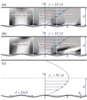
For a laminar Newtonian flow in a plane-Couette geometry with a sinusoidal wavy perturbation on the stationary wall [see schematic diagram in Fig.1(a)], linear analysis has shown that vorticity perturbations induced by the wavy surface can be classified using two non-dimensionalized parameters: (1) the depth of the flow domainα=kdand (2) the viscous length θ = (ηk²/ργ)˙ ^1/3. Here,d is the (dimensional) depth of the domain,kis the wavenumber of the surface undulation,ηis the fluid viscosity,ρis the fluid density, and ˙γis the uniform velocity gradient (shear rate) across the gap.^9,11 Flow configurations withα.1 are considered “shallow,” while those withα&1 are considered “deep.” It can be easily shown that θ=(α²/Re)^1/3, where Re=ργd˙ ²/ηis the Reynolds number, which describes the ratio of inertial to viscous forces. Using

1070-6631/2018/30(11)/113101/10 30, 113101-1 © Author(s) 2018

(4)

FIG. 1. Schematic representation of Couette flow over a wavy surface, indicating the nature of vorticity perturbations predicted in the three regimes of (a) Newtonian and (b) viscoelastic flows.⁹(c) Schematic representation of Poiseuille flow over a wavy surface, as employed in the present study.

these two dimensionless parameters, the vorticity perturbations caused by the wavy surface to the Couette base flow fall into one of three regimes [as illustrated in Fig.1(a)] in theα−θ parameter space, each with characteristic depths of penetration into the flow domainP_ω.^9,11

A “shallow viscous” regime occurs forα.1,θ > α; in this regime, the channel depth is small compared to the roughness wavelength so the vorticity perturbation fills the flow domain (P_ω≈α). The viscous layer is deeper than the flow domain, and so the flow is unaffected by inertia.

A “deep viscous” regime occurs forα&1,θ&1; in this regime, the channel depth is large compared to the roughness wavelength, and the vorticity perturbation decays within the flow domain over approximately one wavelength from the surface (P_ω ≈1). Again, viscosity is dominant and the flow is unaffected by inertia.

Finally, an “inviscid” regime occurs for the conditionsα

> θ,θ.1. In this case, the viscous layer is confined within the flow domain and inertial effects are appreciable. The perturbation is confined within the viscous layer (P_ω∼θ) and is tilted forward due to the inertia.^9,11

Using linear analysis applied to the Oldroyd-B viscoelastic constitutive model, Page and Zaki⁹ studied the effects of fluid elasticity on the vorticity field in the same plane-Couette configuration [Fig.1(b)]. Somewhat in analogy to Newtonian flows, they found that the vorticity perturbations induced by the wavy surface in viscoelastic flows could also be classified using two non-dimensionalized parameters: (1) the depth of the flow domainα= kdand (2) the depth of the “critical layer” Σ = kp2τη_p/ρ. Here, τ is the fluid relaxation time andη_p is the polymer contribution to the fluid viscosity. The critical layer is predicted to occur at the depth where vorticity waves traveling along tensioned mean-flow streamlines prop- agate at the same velocity as the base flow.⁹ It can be shown that the critical layer depth is related to the fluid elasticity by

Σ=kd

√

2El, where the elasticity numberEl= (1− β)Wi/Re.

Here,β=η_s/η₀is the solvent-to-total viscosity ratio (whereη_s is the solvent viscosity andη₀=ηs+ηpis the zero shear viscosity of the fluid), andWi=γτ˙ is the Weissenberg number, which describes the ratio of elastic to viscous forces. Again in analogy with Newtonian flows, three regimes of vorticity perturbations were found [as illustrated in Fig.1(b)],⁹each with characteristic depths of penetrationP_ω.

A “shallow elastic” regime was identified for the condi- tionsα.1,Σ> α. In this regime, the channel depth is small compared to the roughness wavelength, so the vorticity perturbation fills the flow domain (P_ω≈α).^9,11However, the fluid elasticity is high enough such that the critical layer is located outside of the flow domain and so has little influence on the flow.

A “deep elastic” regime was identified for the conditions α & 1, Σ & 1. In this regime, the channel depth is large compared to the roughness wavelength, so the vorticity perturbation decays within the flow domain over approximately one wavelength (P_ω≈1).^9,11However, the critical layer is deeper than the depth of the penetration and so again has little impact on the flow.

While the shallow elastic and deep elastic regimes appear essentially similar to their Newtonian counterparts (shallow viscous and deep viscous, respectively), the third regime predicted for wavy viscoelastic flows contrasts significantly with the third (inviscid) regime observed for Newtonian flow. The so-called transcritical regime was identified for the conditions α >Σ,Σ.1. Here, the critical layer is located both within the flow domainand within the region over which the vorticity perturbation naturally decays. Amplification of the vorticity perturbation takes place at the critical layer, leading to a penetration depth that scales asP_ω∼Σ. The term “transcritical”

is used to describe this regime in order to convey that the base flow velocity varies from “subcritical” near the wavy wall to

“supercritical” at depths beyond the critical layer. The generation of vorticity at the critical layer is explained in terms of a kinematic amplification mechanism due to the polymer torque.⁹

In recent work, we developed experimental methods to test the analytical predictions for the vorticity perturbations found in shear flows over wavy surfaces.^10,16For experimental convenience, a Poiseuille flow was employed in favor of plane-Couette; see Fig.1(c). Five wavy-walled channels were fabricated with a range of 0.6.α.10, and the flow velocimetry in the devices was used to quantify the perturbations based on the measurement of transverse velocity components. Two Newtonian fluids of contrasting viscosity were tested over a range of Re such that the dimensionless viscous length was varied in the range 0.1 . θ . 30. The excellent agreement between the experimental results and linear theory in the same Poiseuille configuration showed that the devices conform to the constraints of linear assumptions and allowed the first experimental verification of the Newtonian flow phase diagram in theα−θparameter space.¹⁶Subsequently, using a weakly viscoelastic polymer solution (El ≈ 0.007) in a deep wavy channel (α≈10,Σ≈1) and by comparison with the linear theory for viscoelastic wavy Poiseuille flows, we demonstrated the first experimental evidence supporting the prediction of

(5)

113101-3 Hawardet al. Phys. Fluids30, 113101 (2018)

the critical layer and hence of the vorticity amplification in the transcritical regime.¹⁰

In the current work, we present an extensive set of experiments utilizing all five of our wavy walled channels (spanning a wide range ofα) and employing a variety of well-characterized polymer solutions with a range of rheological properties providing 0.001 <El <43.6 and hence a range ofΣspanning more than two decades in each channel. We thoroughly inves- tigate the three predicted regimes of wavy viscoelastic shear flow and use our results to construct an experimental phase diagram in theα−Σparameter space that conforms well to the theoretical prediction.

II. MATERIALS AND METHODS A. Flow geometries

The five wavy-walled flow channels used in the experiments are described in detail in a previous publication.¹⁶A schematic representation of the channels, indicating the coor- dinate system and the important dimensions, is provided in Fig.1(c). All of the channels have a total depth 2d= 400µm acrossy, a spanwise width4= 2 mm throughz(aspect ratio r_a=4/2d = 5), and total lengthL= 30 mm alongx. The five channels differ in terms of the wavelength of the wavy surface on the bottom spanwise wall, which is varied in the range 0.125≤λ≤2 mm. The amplitude of the wave isA= 10µm (i.e.A=d/20≤λ/12.5). Due to the small amplitude, the maximum contraction ratio (i.e. between the widest and narrowest sections of channel) isr_c= 410/390≈1.05, and extensional components in the flow field are considered negligible. Indeed, we have shown thatAis small enough to be considered as a linear perturbation to the Poiseuille base state,¹⁶so we consider the flow kinematics to be entirely dominated by simple shear. For convenience, TableI provides the actual parameters of each of the five channels, including the wavenumber of the surfacekand the dimensionless depthα. In this Poiseuille configuration, we consider the depth of the flow domaind to be the region of monotonically increasing flow velocity above the wavy wall (i.e. half the total depth of the channel).

B. Test fluids

A range of viscoelastic polymer solutions are tested in the five wavy channels. The fluids are composed of commer- cially available poly(ethylene oxide) samples (Sigma Aldrich) of molecular weightM= 4 MDa (named PEO4) orM= 8 MDa (named PEO8). Stock solutions are prepared by dissolving the polymer powder at 0.1 wt. % concentration in one of two solvents: either deionized (DI) water or DI water viscosified by the

TABLE I. Salient dimensions of the wavy-walled channels.

Device d(mm) 4(mm) A(µm) λ(mm) k(mm¹) α

1 0.2 2 10 2.0 π 0.2π

2 0.2 2 10 1.25 1.6π 0.32π

3 0.2 2 10 0.4 5π π

4 0.2 2 10 0.25 8π 1.6π

5 0.2 2 10 0.125 16π 3.2π

addition of 13 wt. % of a low molecular weight poly(ethylene glycol) (PEG,M= 8 kDa). At this concentration and molecular weight, the aqueous PEG solution behaves as a Newtonian fluid with a viscosity around 8 times that of water.¹⁷Test fluids are prepared at the desired polymer concentrations 0.001≤c≤ 0.05 wt. % by dilution of the stock solution in the appropriate quantity of the respective solvent.

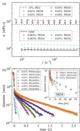
The viscosities of the test fluids (and the two solvents) were measured at 25^◦C using a DHR3 stress-controlled rota- tional rheometer (TA Instruments, Inc.) fitted with a 40 mm diameter 1^◦cone-and-plate fixture and the results are shown in Fig.2(a). The measured viscosities of the two solvents are η_s = 0.87 mPa s (DI water) andη_s = 7.72 mPa s (13 wt. % PEG). The zero shear viscositiesη₀of the polymer solutions are all quite close to the viscosity of their respective solvent (i.e. the viscosity ratio βis in general close to unity), and the fluids do not exhibit significant shear thinning.

The densities of the polymer solutions are taken to be equal to those of their solvents, which were measured at 25^◦C by weighing various volumes of fluid dispensed from calibrated micropipettes, yielding ρ = 996.9 kg m⁻³ and ρ= 1015.5 kg m⁻³ for the pure DI water and the 13 wt. % PEG, respectively.

The relaxation times τ of the polymer solutions were determined by measurements made in a capillary breakup extensional rheometer (CaBER 1, Thermo Haake).^19,20In this method, an initially cylindrical fluid sample is held by surface tension between two axially aligned circular end plates

FIG. 2. (a) Rheological characterization of the viscoelastic test solutions and their solvents at 25^◦C in steady shear in a DHR3 stress-controlled rheometer (TA Instruments, Inc.) equipped with a 40 mm diameter 1^◦angle cone-and- plate geometry. (b) Capillary thinning measurements performed in a CaBER device in order to assess the fluid relaxation times. Inset shows data obtained for the most weakly elastic fluids using the slow retraction method (SRM).¹⁸

(6)

(diameterD₀= 6 mm, initial separationl₀= 1 mm). At time t₀=−50 ms, the end plates are displaced axially at a relative rate of 0.1 m s⁻¹ to reach a final separation ofl₀ = 6 mm at timet = 0 s. A laser micrometer located at the midpoint between the endplates in their final position monitors the diam- eterD(t) of the liquid bridge as it thins due to capillary forces.

For Newtonian fluids, the liquid bridge thins linearly with time at a viscosity-dependent rate.²¹However, an elongational flow is set up within the necking liquid bridge, which for polymer solutions causes alignment of polymer molecules and the generation of elastic forces that retard the capillary-driven thinning process. Under these conditions of elasto-capillarity, the filament diameter decays exponentially with time as D∼exp(−t/3τ).^19,20Figure2(b)shows the filament diameter as a function of time measured for the various polymer solutions, each showing a clear exponentially decaying region from which the relaxation time is extracted. For the most dilute fluids in the DI water solvent, the filament thinning was too rapid to resolve accurately using the standard CaBER setup. For these fluids, we employed the slow retraction method (SRM) to generate the fluid filament,¹⁸ and we used a high speed Phantom Miro camera (Vision Research, Inc.) rather than a laser micrometer in order to monitor the decay of the filament diameter over time. The results from these SRM tests are shown in the inset to Fig.2(b), again demonstrating clear elasto-capillary regions from which the relaxation time can be extracted. Note that one particular test fluid (0.01 wt. % PEO4 in DI water) was tested using both standard CaBER and the SRM technique, with reasonably good agreement obtained for the relaxation time in each case (τ = 12 ms by CaBER and τ= 14 ms by SRM).

TableIIprovides the salient rheological parameters of all viscoelastic test fluids employed in the flow experiments.

C. Dimensionless flow parameters

Flow of the test fluids through the wavy channels is driven at a controlled volume flow rate Q using a neMESYS low pressure syringe pump (Cetoni GmbH) fitted with a Hamilton Gastight glass syringe connected to the channel using silicone tubing. The average flow velocity in the channel along thex- direction [Fig.1(b)] is thenU =Q/2wd. Note that based on the vorticity and polymer torque equations used in the linear

theory, we do not expect results to differ depending on whether the flow is driven at controlled rate or controlled pressure.^9,10 As a characteristic shear rate, we take the nominal velocity gradient at the wall for Newtonian flow ˙γ_w =3U/d. Since in the Poiseuille configuration, the total channel depth is 2d, the Reynolds number becomes

Re=2ρUd

η =2ργ˙_wd²

3η . (1)

The Weissenberg number is given as usual by

Wi=γ˙_wτ, (2)

and hence the elasticity number is El=(1−β)Wi

Re= 3η_pτ

2ρd². (3)

The dimensionless viscous length in the wavy Poiseuille configuration is given by

θ= ηk² ργ˙_w

!^1/3

= 2α² 3Re

!^1/3

, (4)

and the dimensionless critical layer depth becomes Σ=k

s2η_pτ ρ =kd

r4El

3 . (5)

Apart from some numerical factors arising from the def- initions of Re and ˙γ_w, bothθ andΣin the wavy Poiseuille flow are entirely equivalent to those used in the wavy Couette case. A difference between the two configurations arises in the classification of deep and shallow channels. Experiments and linear theory with Newtonian fluids in wavy Poiseuille flow have shown that channels with α . π are to be considered shallow and those withα&πshould be considered deep.¹⁶

As shown in TableII, by virtue of using two solvents of contrasting viscosities and by varying the polymer molecular weight and concentration, the viscoelastic test fluids span a wide range of elasticity 0.001 ≤El ≤43.6. However, the solvent-to-total viscosity ratio is kept high (β≥0.69), thereby avoiding complications associated with shear thinning (i.e. rate dependence ofτandη, hence Re,Wi,θandΣ, and rate dependent base flow profiles in the channels). For a given fluid and elasticity number, the value ofΣdepends on the wavelength

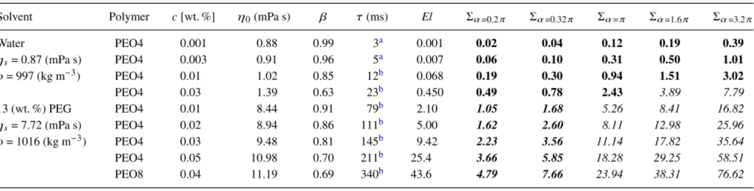
TABLE II. Composition and material parameters of the experimental test fluids at 25^◦C, including the values ofΣfor each fluid in each channel. Bold-italic indicates expected shallow elastic, italic indicates expected deep elastic, and bold indicates expected transcritical behavior.

Solvent Polymer c[wt. %] η0(mPa s) β τ(ms) El Σ_α=0.2π Σ_α=0.32_π Σ_α=_π Σ_α=1.6π Σ_α=3.2π

Water PEO4 0.001 0.88 0.99 3^a 0.001 0.02 0.04 0.12 0.19 0.39

ηs= 0.87 (mPa s) PEO4 0.003 0.91 0.96 5^a 0.007 0.06 0.10 0.31 0.50 1.01

ρ= 997 (kg m³) PEO4 0.01 1.02 0.85 12^b 0.068 0.19 0.30 0.94 1.51 3.02

PEO4 0.03 1.39 0.63 23^b 0.450 0.49 0.78 2.43 3.89 7.79

13 (wt. %) PEG PEO4 0.01 8.44 0.91 79^b 2.10 1.05 1.68 5.26 8.41 16.82

ηs= 7.72 (mPa s) PEO4 0.02 8.94 0.86 111^b 5.00 1.62 2.60 8.11 12.98 25.96

ρ= 1016 (kg m³) PEO4 0.03 9.48 0.81 145^b 9.42 2.23 3.56 11.14 17.82 35.64

PEO4 0.05 10.98 0.70 211^b 25.4 3.66 5.85 18.28 29.25 58.51

PEO8 0.04 11.19 0.69 340^b 43.6 4.79 7.66 23.94 38.31 76.62

aRelaxation time measured using the slow retraction method (SRM).

bRelaxation time measured using the standard CaBER technique.

(7)

of the surface undulation of the channel. TableIIprovides the values ofΣfor each fluid at each value ofα. It can be seen by inspection of Eq.(5) thatEl ≤0.75 for transcritical phe- nomena to be observed (since it is required thatΣ/α≤1). In TableII,Σ–αcombinations that correspond to expectations for transcritical behavior in wavy Poiseuille flow are identified by bold text. The remainingΣ–αcombinations are listed in either bold-italic or italic text in order to identify expected shallow elastic (α < π) or deep elastic (α≥π) behavior, respectively.

D. Micro-particle image velocimetry (µ-PIV)

Perturbations to the Poiseuille base flow state caused by the wavy surfaces are characterized by measuring velocity vector fields within the wavy channels using a micro-particle image velocimetry (µ-PIV) system (TSI, Inc.). The fluids are seeded with 1µm diameter fluorescent microparticles (nile red FluoSpheres, Life Technologies) with excitation and emission wavelengths of 535 and 575 nm, respectively. The flow channel is placed on the imaging stage of an inverted microscope (Nikon Eclipse Ti), and the mid-plane of the device (z=4/2) is brought into focus. The measurement section of the test channel commences at a distance of∆x≈18 mm (∆x/2d ≈45) downstream of the inlet, allowing adequate distance for the flow to become fully developed. Depending on the particular flow channel being studied, objective lenses are selected in order to maximize the spatial resolution of the measurement while simultaneously allowing at least one full wavelength of the undulation, and the full depth of the flow domain, to be visualized. Accordingly, for Devices 1 and 2 (with the longest wavelengths), a 4×NA = 0.13 objective is required; for Device 3 a 5×NA = 0.15 objective is used; and for Devices 4 and 5 (with the shortest wavelengths), a 10×NA = 0.3 objective is employed. The corresponding measurement width, over which microparticles contribute to the determination of velocity vectors, is δz_m≈142, 109 and 31 µm for the 4×, 5×and 10× lenses, respectively.²²Even in the worst case of the 4×objective lens,δz_mis only≈7% of the channel width, so there should not be a significant measurement error given the high channel aspect ratios and therefore the expected uniform flow along thez-direction close to the mid-plane. The fluid is illuminated through the microscope objective by a dual-pulsed Nd:YLF

laser at 527 nm, exciting the fluorescent particles. The light emitted by the particles is imaged through the same objective lens, passed through a G2-A epifluorescent filter, and projected onto the sensor array of a high speed Phantom Miro camera (Vision Research, Inc.), operating in the frame-straddling mode. Images are captured in pairs, in synchronicity with the pairs of laser pulses. The time between laser pulses∆tis cho- sen such that the maximum particle displacement between images in each pair is around 8 pixels, optimal for the standard cross-correlation PIV algorithm used to obtain velocity vectors based on a square grid of 32×32 pixel interrogation areas. Since in this work we are only interested in examining steady flows, at each flow rate imposed in each device, vector fields are ensemble-averaged over the data from up to 50 image pairs. In cases where more than one wave of the surface is visualized, the fully developed nature of the flow over the measurement section is clearly evident from the cyclic variation in the velocity field from wave to wave. In such cases, in order to further reduce noise, the data are also averaged over successive waves.

Velocity vector fields measured in thex–yplane atz=4/2 have componentsuandv in thex- andy-directions, respectively. Since for the Poiseuille base flow (i.e. if there were no wavy surface)v_Pois≡0, our measurement ofvallows a simple and direct determination of the perturbation componentv⁰=v

−v_Pois≡v. As we have shown, thisv⁰component is sufficient to characterize the perturbation, without the need to resort to any assumptions or approximations that are necessary in order to extract theu⁰ perturbation component from the data and thus to evaluate the full vorticity perturbationω⁰=∂v⁰/∂x−

∂u⁰/∂y.¹⁶Hence, in this work (as in our previous work), we use v⁰rather thanω⁰to evaluate an experimental measure of the penetration depth of the disturbance. For this measure, which we denoteP_v, we employ a criterion similar to that proposed by Page and Zaki:^9,10

P_v ≡ky(Λ_v=0.95), whereΛ_v(y)= _y

0

|v⁰(s)|²ds

_d

0

|v⁰(s)|²ds , (6)

where |v⁰(y)| is averaged over the full range ofxin the field of view.

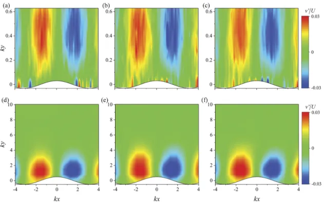
FIG. 3. Three regimes of viscoelastic Poiseuille flow in wavy-walled microchannels atWi≈40: (a) shallow elastic regime (α < π,Σ> α), for the flow of the 0.04 wt. % solution of PEO8 in Device 2 (α= 0.32π,Σ= 7.66,β= 0.69, Re = 0.29), (b) deep elastic regime (α > π,Σ> π), for the flow of the 0.04 wt. % solution of PEO8 in Device 4 (α= 1.6π,Σ= 38.31,β= 0.69, Re = 0.29), (c) and transcritical regime (α >Σ,Σ< π), for the flow of the 0.01 wt. % solution of PEO4 in Device 4 (α= 1.6π,Σ= 1.51,β= 0.85, Re = 87.15).

(8)

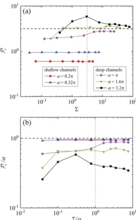
FIG. 4. Penetration ofv⁰perturbations atWi≈40 in all five wavy test channels: (a)P_v as a function ofΣ; the horizontal dashed line marksP_v = π and the vertical dotted line marksΣ=π. (b)P_v/αas a function ofΣ/α;

the horizontal dashed line marksP_v =αand the vertical dotted line marks Σ=α.

III. RESULTS

As predicted by linear theory for viscoelastic wavy plane- Couette flow,⁹ three broad regimes of viscoelastic flow can also be observed in the flow patterns measured experimentally in the wavy-walled channels. These three regimes, with parametersαandΣcorresponding to the expectations of shallow elastic, deep elastic and transcritical type behavior, are illustrated in Figs.3(a),3(b), and3(c), respectively. As will be shown in detail subsequently, the flow patterns in the shallow and deep elastic regimes are essentially Newtonian-like

in appearance; the perturbation extends straight along they- direction and penetrates all the way through the flow domain in the shallow channel [Device 2, Fig.3(a)], but decays over a dimensionless depth of≈3 in the deep channel [Device 4, Fig.3(b)]. In the transcritical regime [Fig.3(c), also shown for Device 4], the perturbation is clearly intensified compared with that in Fig.3(b), is markedly tilted forward and also penetrates more deeply into the channel.

In Fig.4we present the penetration depth measurements [evaluated according to Eq. (6)] made in all five wavy wall test channels (0.2π ≤ α≤3.2π) with all the test fluids (i.e.

for a range ofΣ). Following the analysis performed by Page and Zaki,⁹ the data are plotted for a relatively high value of the Weissenberg numberWi≈40. The reason for this particular choice ofWiis that it is the highest value that could be achieved with all of the fluids in all of the channels. For fluids with short relaxation times, obtaining higherWiwas not fea- sible due to the high flow velocities required and constraints on theµ-PIV imaging rate. On the other hand, for more elastic fluids with longer relaxation times, higherWiflows resulted in elasticity-driven recirculations in the troughs of the wavy surface (particularly in channels with shorter wavelengths). These recirculations can be seen by observing the motion of individual µ-PIV tracer particles at different times, as illustrated for one particular case in Fig.5 (multimedia view). Figure4(a) showsP_v as a function ofΣ. Here it can be seen that for the higher values of Σin each channel (i.e. towards the elastic limit), a region of approximately constantP_vis reached. This highΣplateau appears to reach an asymptotic valueP_v ≈3 (or π, marked by the horizontal dashed line) forα≥5, thus indicating deep elastic behavior. Figure4(b)showsP_v/αas a function ofΣ/α. In this plot, it can be seen that the plateau ofΣ/αasymptotes to a value of approximately 1 (i.e.Σ=α, marked by the horizontal dashed line) forα≤1, thus indicating shallow elastic behavior. These two regimes are highly anal- ogous to deep viscous behavior and shallow viscous behavior reported previously for Newtonian fluids.¹⁶

For deep channels only (i.e. α≥ π), the plots in Fig.4 show a change in behavior forΣ.π,Σ/α.1, marking the expected boundary between the transcritical and deep elastic regimes (indicated by the vertical dotted lines in the two plots).

FIG. 5. [(a)–(d)] Illustration of recirculations observed in the troughs of a deep wavy channel (α= 3.2π) during flow of the fluid withΣ= 58.51 atWi≈127 by observing individualµ-PIV tracer particles. The bulk flow is from left to right. Two particular particles are identified in the central trough, outlined by red and yellow circles and with their directions of motion indicated by the correspondingly colored arrows. Multimedia view:

https://doi.org/10.1063/1.5057392.1

(9)

At the change in regime between deep elastic and transcritical behavior, we note several similarities between our experimental data and the theoretical plots presented by Page and Zaki (in their case forWi= 60).⁹In particular, in the deepest channel (α= 3.2π), there is a significant overshoot inP_vasΣincreases and the flow regime transitions into the deep elastic. Also, in the shallower (α = 1.6π) channel, the plateau region of P_v extends further into the transcritical regime (i.e. to lowerΣ).

However, the channel withα=πexhibits contrasting behavior, and no clear or general scaling betweenΣandP_vis evident for the three deep channels in the transcritical region. We note here that we do not expect to see evidence of transcritical behavior in the shallow channels (α < π) since the perturbation spans the entire flow domain under all imposed conditions. For the same reason, we also could not observe inviscid type behavior in shallow channels in our experiments with Newtonian fluids.¹⁶

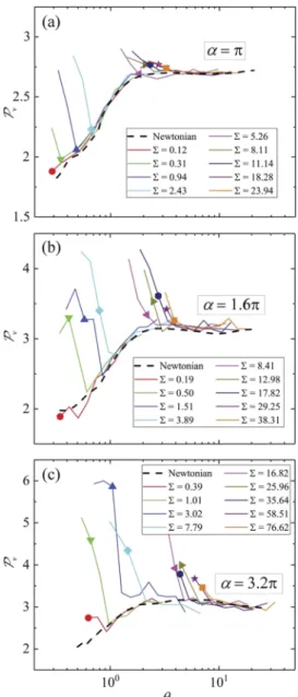
Focusing only on deep channels (α ≥π), we can obtain some insight into the absence of a transcritical scaling forP_v withΣin Fig.4by examining how the penetration depth for the viscoelastic fluids depends on the imposed flow conditions. In Figs.6(a)–6(c)we present the penetration depth as a function of the viscous lengthθmade for all the viscoelastic test fluids and shown in comparison with the results obtained for Newtonian flow. The Newtonian behavior is indicated by the dashed black curves, while the colored curves show the responses of the various polymer solutions. The solid colored data points mark the conditions whereWi= 40 (i.e. the data shown previously in Fig. 4). These plots clarify several key points. At low flow rates (i.e. lowWi, low Re and hence highθ), the polymer solutions all appear Newtonian-like, with the penetration depth lying on the high-θ plateau. The polymer solution responses closely follow the Newtonian curves asθ is decreased (i.e. asWiand Re increase) until a sudden depar- ture from Newtonian behavior is seen at aΣ-dependent value of θ, where P_v dramatically increases. The most significant excursions from Newtonian behavior are seen for the polymer solutions that follow the Newtonian curves into the sloping (inviscid) region, which are in general the same fluids expected to show transcritical behavior. This indicates the importance of the combination of both inertia and elasticity for the clear manifestation of the transcritical regime.

It is evident from Figs. 6(a)–6(c)that by selecting penetration depth measurements from all of the test fluids and channels at a single fixed value of the Weissenberg number (as in Fig. 4 atWi= 40), the different regions of the phase diagram are not being compared under equivalent conditions in all of the channels. It is clear in Fig.6(a)that atWi= 40 in theα=πchannel, the response is close to Newtonian for all Σ. On the other hand, atWi= 40 in theα= 1.6πandα= 3.2π channels [Figs.6(b)and6(c), respectively], a significantly non- Newtonian response is recorded. These observations explain the absence of a clear and general scaling betweenP_vandΣ observed within the transcritical regime for the data shown in Fig.4.

A. Shallow elastic and deep elastic regimes

In this section, we provide additional details of the appearance of thev⁰perturbation patterns observed within the shallow

FIG. 6. Penetration depth ofv⁰perturbations as a function ofθin deep wavy channels: (a)α=π, (b)α= 1.6π, and (c)α= 3.2π. The dashed black lines show the result obtained using Newtonian fluids, while the colored lines show the trajectories of the various polymer solutions. The solid symbols mark the location ofWi= 40 for each of the polymer solutions.

elastic and deep elastic regimes. Both of these regimes are anticipated to resemble the Newtonian response and are hence reported only briefly.

The top panel of Fig. 7 shows v⁰ perturbation patterns observed in the shallow elastic regime in Device 1 (α= 0.2π).

In Fig.7(a)we show the result obtained for a Newtonian fluid (13 wt. % PEG) in the shallow viscous regime (α < π,θ > α).

In Figs.7(b)and7(c)we show examples of the shallow elastic regime (α < π,Σ > α) for two different polymer solutions (Σ = 2.23 and Σ = 3.66) at Wi ≈ 40. The two polymeric fluids here demonstrate negligible difference from the behavior of the Newtonian fluid in the shallow viscous regime; in all three cases, the perturbation is of similar magnitude and extends straight along they-direction completely across the flow domain.

The bottom panel of Fig.7shows the nature ofv⁰perturbation patterns observed in the deep elastic regime in Device 5

(10)

FIG. 7. v⁰perturbation patterns observed in the elastic regime compared with a low Re Newtonian flow. Top panel: Device 1 (α= 0.2π) with (a) Newtonian fluid (13 wt. % PEG) at Re = 0.62,θ= 0.75 (i.e. shallow viscous regime), (b) 0.03 wt. % solution of PEO4 in 13 wt. % PEG (Σ= 2.23) atWi≈40,θ= 0.69, and (c) 0.05 wt. % solution of PEO4 in 13 wt. % PEG (Σ= 3.66) atWi≈40,θ= 0.82. Bottom panel: Device 5 (α= 3.2π) with (d) Newtonian fluid (13 wt. % PEG) at Re = 0.35,θ= 5.79 (i.e. deep viscous regime), (e) 0.05 wt. % solution of PEO4 in 13 wt. % PEG (Σ= 58.5) atWi≈40,θ= 5.23, and (f) 0.04 wt. % solution of PEO8 in 13 wt. % PEG (Σ= 76.6) atWi≈40,θ= 6.17.

(α = 3.2π). For comparison with the polymeric flow, in Fig.7(d)we show the result for a Newtonian fluid (13 wt. % PEG) in the deep viscous regime (α > π,θ >1). In Figs.7(e) and7(f), we show examples of the deep elastic regime (α > π, Σ > π) for two different polymer solutions (Σ = 58.5 and Σ = 76.6) atWi ≈40. The two polymeric fluids here again demonstrate only a minor difference from the behavior of the Newtonian fluid, with the perturbation having a similar magnitude and only penetrating slightly more deeply into the channel.

B. Transcritical regime

In this section, we provide additional details on the observations of flow patterns within the transcritical flow regime (α >Σ,Σ< π) in the deep wavy channels (α≥π).

The top panel of Fig.8shows details ofv⁰perturbation patterns observed in the transcritical regime in Device 3 (α

=π), as the Weissenberg and Reynolds numbers are progressively increased for a fixedΣ= 0.94. AtWi= 40 [Fig.8(a)], the response is essentially that of a Newtonian fluid in the inviscid regime [as established in Fig.6(a)]. Due to the small viscous length (θ = 0.42), the perturbation is localized close to the wavy wall and is notably tilted forward by the shear. As the Weissenberg number is increased toWi= 71.4 andWi= 127.0 in Figs.8(b)and8(c), respectively, the perturbation remains tilted forward but also increases substantially in magnitude and penetrates progressively more deeply into the channel (even though the viscous lengthθactually decreases).

The middle panel of Fig. 8 shows details of v⁰ perturbation patterns observed in the transcritical regime in Device

4 (α = 1.6π) at a fixedΣ = 1.51. As the Weissenberg and Reynolds numbers are progressively increased through Figs.8(d)–8(f), similar observations can be made as described above for Device 3.

The bottom panel of Fig. 8 shows details of v⁰ perturbation patterns observed in the transcritical regime in Device 5 (α= 3.2π). Here, the Weissenberg number is held fixed at Wi≈40 as the value ofΣis progressively increased through Figs.8(g)–8(i). At lowΣ= 0.39 [Fig.8(g)], the perturbation is quite intense, tilted forward and localized close to the wavy surface due to a combination of both the small viscous length (θ= 0.55) and the low depth of the critical layer (Σ= 0.39).

In Fig.8(h), the viscous length remains quite small (θ= 0.80), but the increased depth of the critical layer (Σ= 1.01) results in the perturbation penetrating more deeply into the channel while remaining tilted forward. Finally, in Fig.8(i),θ= 0.92 andΣ= 3.02; now the inertia is becoming less significant and the critical layer is located near the deep limit. The flow is tran- sitioning from the transcritical into the deep elastic regime; the perturbation consequently decreases in intensity and becomes straighter and more aligned along they-direction.

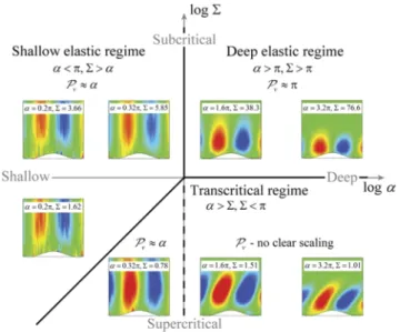
C. Construction of the “phase diagram”

Using the results of our experiments in five different wavy microchannels (providing a range of 0.2π≤α≤3.2π) using nine distinct viscoelastic fluids (providing a range of 0.001≤El ≤43.6, hence a range of critical layer depthsΣ), we can construct an experimental phase diagram in theα−Σ parameter space delineating the flow regimes observed for viscoelastic wavy Poiseuille flow. This phase diagram is shown

(11)

FIG. 8. v⁰perturbation patterns observed in the transcritical regime. Top panel: Device 3 (α=π) with the 0.01 wt. % solution of PEO4 in water (Σ= 0.94) as the Weissenberg number is varied: (a)Wi= 40.1, Re = 87.1,θ= 0.42, (b)Wi= 71.4, Re = 155.0,θ= 0.35, and (c)Wi= 127.0, Re = 275.9,θ= 0.29. Middle panel: Device 4 (α= 1.6π) with the 0.01 wt. % solution of PEO4 in water (Σ= 1.51) as the Weissenberg number is varied: (d)Wi= 22.6, Re = 49.0,θ= 0.70, (e)Wi= 40.1, Re = 87.1,θ= 0.58, and (f)Wi= 71.4, Re = 155.0,θ= 0.48. Bottom panel: Device 5 (α= 3.2π) at fixedWi≈40 as the value ofΣis varied: (g) 0.001 wt. % PEO4 in water (Σ= 0.39, Re = 405,θ= 0.55), (h) 0.003 wt. % PEO4 in water (Σ= 1.01, Re = 131,θ= 0.80), and (i) 0.01 wt. % PEO4 in water (Σ= 3.02, Re = 87.1,θ= 0.92).

in Fig.9 and is in broad agreement with our stateda priori expectations based on the predictions from linear theory using the Oldroyd-B model in a wavy plane-Couette flow⁹ and our earlier experimental work with Newtonian fluids in wavy Poiseuille flow.¹⁶

The theory, applied to plane-Couette flow, predicts transition between the shallow and deep regimes at α = 1 and between the deep elastic and transcritical regimes at Σ= 1.

The experiments, conducted in Poiseuille flow, find these two boundaries atα=πandΣ=π, respectively. Given the assumptions involved in the theory (i.e. Oldroyd-B model, linear perturbation modelled by wall slip), the relative complexity of the experiments (i.e. real viscoelastic fluids with polydis- perse polymer samples, real wavy walls, and measurement uncertainty) and the contrasting flow configurations, the level of agreement is remarkable.

In the shallow elastic and deep elastic regimes, the penetration is exactly as expected (P_v ≈αandP_v ≈ π, respectively). In the transcritical regime, linear theory predicts the

FIG. 9. Experimental phase diagram in theα−Σparameter space, delineating the three regimes observed for viscoelastic wavy Poiseuille flow.

(12)

penetration depth (based on the full vorticity perturbation) to scale asP_ω∼Σ.⁹In our case, using a penetration depth based onv⁰, we divide the transcritical regime into two subregimes (as we also subdivided the inviscid regime for Newtonian flows¹⁶). In the shallow transcritical subregimeP_v ≈α(effec- tively indistinguishable from the shallow elastic behavior). The transition between the deep elastic regime and the deep transcritical subregime is clearly apparent in the observed flow patterns through a marked increase in intensity, a forward tilt of thev⁰perturbation and an increase in the penetration depth.

However, in this work, we find no clear scaling forP_vwithΣ, so we are unable to provide an experimental verification for the theoretical scaling.

IV. DISCUSSION AND CONCLUSIONS

In this work we used a series of five wavy-walled channels and nine polymer solutions of distinct rheology in order to per- form an experimental investigation of viscoelastic shear flows over wavy surfaces. The five channels are all similar except for having distinct ratios of depth to undulation wavelength, α. The channels span the shallowα < πto deepα≥πregimes and have been validated against linear theory in previous work using Newtonian fluids. The polymeric fluids have been formulated to span a wide range of elasticity numbers 0.001≤El

≤43.6, hence a range of dimensionless critical-layer depths Σ ∼√

Elspanning two orders of magnitude in each channel.

The flow patterns observed in our experiments show clear evidence of the three flow regimes (shallow elastic, deep elastic, and transcritical) predicted by linear theory, which fit into the predicted phase diagram in the α−Σ parameter space. This constitutes the first experimental verification of the predicted phase diagram. This provides strong evidence for the existence of the predicted “critical layer” where amplification of the perturbation occurs away from the site of vorticity injection (i.e. away from the wavy surface). In the transcritical regime (which is characterized by a combination of inertia and elasticity), this amplification results in a non-Newtonian increase in the penetration depth above that observed for Newtonian fluids under comparable inertial conditions.

The wavy-wall model studied here is a canonical surrogate to a number of important flows, e.g. the motion of a viscoelastic fluid near a deformable substrate or two-fluid interface, the onset and structure of inertial instabilities, or the flow dynamics in the vicinity of differently sized eddies in elasto-inertial and drag-reduced turbulent flows.

ACKNOWLEDGMENTS

S.J.H. and A.Q.S. gratefully acknowledge the support of the Okinawa Institute of Science and Technology Gradu- ate University (OIST) with subsidy funding from the Cabinet Office, Government of Japan. S.J.H. and A.Q.S. also acknowledge funding from the Japan Society for the Promotion of Science [Grants-in-Aid for Scientific Research (C), Grant

Nos. 18K03958 and 17K06173, and Grants-in-Aid for Sci- entific Research (B), Grant No. 18H01135]. Kazumi Toda- Peters from OIST is thanked for device fabrication. S.J.H. is very grateful to TA Instruments for the donation of a DHR3 rheometer under their Distinguished Young Rheologist Award scheme.

1C. S. Dutcher and S. J. Muller, “Effects of weak elasticity on the stability of high Reynolds number co-and counter-rotating Taylor-Couette flows,”

J. Rheol.55, 1271–1295 (2011).

2N. Burshtein, K. Zografos, A. Q. Shen, R. J. Poole, and S. J. Haward,

“Inertioelastic flow instability at a stagnation point,”Phys. Rev. X7, 041039 (2017).

3D. Samanta, Y. Dubief, M. Holzner, C. Sc¨afer, A. N. Morozov, C. Wagner, and B. Hof, “Elasto-inertial turbulence,”Proc. Natl. Acad. Sci. U. S. A.110, 10557–10562 (2013).

4A. Agarwal, L. Brandt, and T. A. Zaki, “Linear and nonlinear evolution of a localized disturbance in polymeric channel flow,”J. Fluid Mech.760, 278–303 (2014).

5S. J. Lee and T. A. Zaki, “Simulations of natural transition in viscoelastic channel flow,”J. Fluid Mech.820, 232–262 (2017).

6P. S. Virk and H. Baher, “The effect of polymer concentration on drag reduction,”Chem. Eng. Sci.25, 1183–1189 (1970).

7C. M. White and M. G. Mungal, “Mechanics and prediction of turbulent drag reduction with polymer additives,”Annu. Rev. Fluid. Mech.40, 235–256 (2008).

8M. D. Graham, “Drag reduction and the dynamics of turbulence in simple and complex fluids,”Phys. Fluids26, 101301 (2014).

9J. Page and T. A. Zaki, “Viscoelastic shear flow over a wavy surface,”

J. Fluid Mech.801, 392–429 (2016).

10S. J. Haward, A. Q. Shen, J. Page, and T. A. Zaki, “Inertioelastic Poiseuille flow over a wavy surface,”Phys. Rev. Fluids3, 091302 (2018).

11F. Charru and E. J. Hinch, “‘Phase diagram’ of interfacial instabilities in a two-layer Couette flow and mechanism of the long-wave instability,”

J. Fluid Mech.414, 195–223 (2000).

12M. K. S. Verma and V. Kumaran, “A multifold reduction in the transition Reynolds number, and ultra-fast mixing, in a micro-channel due to a dynamical instability induced by a soft wall,”J. Fluid Mech.727, 407–455 (2013).

13V. Kumaran and P. Bandaru, “Ultra-fast microfluidic mixing by soft-wall turbulence,”Chem. Eng. Sci.149, 156–168 (2016).

14P. Laure, H. Le Meur, Y. Demay, J. C. Saut, and S. Scotto, “Linear stability of multilayer plane Poiseuille flows of Oldroyd B fluids,”J. Non-Newtonian Fluid Mech.71, 1–23 (1997).

15B. Khomami and K. C. Su, “An experimental/theoretical investigation of interfacial instabilities in superposed pressure-driven channel flow of Newtonian and well characterized viscoelastic fluids Part I: Linear stability and encapsulation effects,”J. Non-Newtonian Fluid Mech.91, 59–84 (2000).

16S. J. Haward, A. Q. Shen, J. Page, and T. A. Zaki, “Poiseuille flow over a wavy surface,”Phys. Rev. Fluids2, 124102 (2017).

17P. Dontula, C. W. Macosko, and L. Scriven, “Model elastic liquids with water-soluble polymers,”AIChE J.44, 1247–1255 (1998).

18L. Campo-Dea˜no and C. Clasen, “The slow retraction method (SRM) for the determination of ultra-short relaxation times in capillary breakup extensional rheometry experiments,”J. Non-Newtonian Fluid Mech.165, 1688–1699 (2010).

19V. M. Entov and E. J. Hinch, “Effect of a spectrum of relaxation times on the capillary thinning of a filament of elastic liquid,”J. Non-Newtonian Fluid Mech.72, 31–54 (1997).

20S. L. Anna and G. H. McKinley, “Elasto-capillary thinning and breakup of model elastic liquids,”J. Rheol.45, 115–138 (2001).

21D. T. Papageorgiou, “On the breakup of viscous liquid threads,”Phys. Fluids 7, 1529–1544 (1995).

22C. D. Meinhart, S. T. Wereley, and M. H. B. Gray, “Volume illumination for two-dimensional particle image velocimetry,”Meas. Sci. Technol.11, 809–814 (2000).