A gl obal m
ul t i - s ec t or al m
odel i n l oc al
c ur r enc i es
著者
Yano Takas hi
権利
Copyr i ght s 日本貿易振興機構(ジェトロ)アジア
経済研究所 / I ns t i t ut e of D
evel opi ng
Ec onom
i es , J apan Ext er nal Tr ade O
r gani z at i on
( I D
E- J ETRO
) ht t p: / / w
w
w
. i de. go. j p
j our nal or
publ i c at i on t i t l e
I D
E D
i s c us s i on Paper
vol um
e
703
year
2018- 03
INSTITUTE OF DEVELOPING ECONOMIES
IDE Discussion Papers are preliminary materials circulated
to stimulate discussions and critical comments
Keywords:
global multi-country model; exchange rate; local currencyJEL classification:
C54; D57; D58; F47* Senshu University, E-mail: [email protected]
IDE DISCUSSION PAPER No. 703
A Global Multi-Sectoral Model in
Local Currencies
Takashi YANO*
March 2018
Abstract
The Institute of Developing Economies (IDE) is a semigovernmental,
nonpartisan, nonprofit research institute, founded in 1958. The Institute
merged with the Japan External Trade Organization (JETRO) on July 1, 1998.
The Institute conducts basic and comprehensive studies on economic and
related affairs in all developing countries and regions, including Asia, the
Middle East, Africa, Latin America, Oceania, and Eastern Europe.
The views expressed in this publication are those of the author(s). Publication does not imply endorsement by the Institute of Developing Economies of any of the views expressed within.
INSTITUTE OF DEVELOPING ECONOMIES (IDE), JETRO 3-2-2, WAKABA,MIHAMA-KU,CHIBA-SHI
CHIBA 261-8545, JAPAN
©2018 by Institute of Developing Economies, JETRO
1
A Global Multi-Sectoral Model in Local Currencies
Takashi Yano
*Abstract
Economic agents make their decisions by focusing on the economic performance of their economies in their currencies rather than in a foreign currency. This shows that a multi-country economic model in local currencies is suitable to analyze global economic issues. However, international input-output tables are denominated in a specific currency such as the US dollar. Employing the OECD Intercountry Input-Output Tables, this paper presents a method to convert the international input-output tables in U.S. dollars and current prices to those in local currencies and constant prices. In addition, the structure of a global model with economies of scale and imperfect competition is illustrated. A numerical example is also demonstrated in order to show the applicability of the model.
Keywords: global multi-country model; exchange rate; local currency JEL code: C54; D57; D58; F47
1.
Introduction
This paper aims at developing a new approach for global economic modeling; specifically, a local currency-based global multi-sectoral model.
The history of the world economy shows that economic interdependence of nations has been strengthened through trade and investment. Project LINK is a pioneering macroeconometric model which describes a global economy in the context of economic interdependence. Subsequently, many institutions and scholars construct multi-county macroeconometric models such as the International Monetary Fund’s Global Economy Model (Pesenti, 2008), Fair’s (1994) Multi-Country Model, Taylor’s (1993) Multi-Country Model. However, recent economic deregulation enables firms to investment overseas. In fact, firm-level foreign direct investment is growing rapidly. Therefore, macroeconometric models are not necessarily adequate for global economic analysis. Instead, a global model at sector level is more appropriate for analyzing the current world economy. Regarding multi-country multi-sectoral models, the following four types of models have been developed: 1) computable general equilibrium (CGE) model such as the Michigan model (Deardorff and Stern, 1986), the GTAP model (Hertel, 1996) and the G-Cubed
2
model (McKibbin and Wilcoxen, 1999) , 2) the INFORUM system which interlinks national input-output models with a trade linkage model (Almon, 1991; Uno, 2002), 3) single-period international input-output model (Torii et al. 1989; Kosaka, 1994; Yano and Kosaka, 2003), and 4) price-linked multi-country multi-sectoral model (Yano and Kosaka, 2015). However, the first three models have shortcomings: a typical CGE model lacks statistical foundations of parameters; the INFORUM system might have inconsistency between classifications in input-output tables and trade matrix; a single-period international input-output model has limitations in specifications and estimation of behavioral equations due to the use of only a single-period international input-output table. A price-linked multi-country multi-sectoral model improves the flaws of these three models, yet it has a drawback: that is, a currency problem. The model in Yano and Kosaka (2015) is denominated in international dollars. In reality, however, economic agents make their decisions by focusing on economic performance of their economies in their currencies rather than a foreign currency. In addition, it is quite difficult to include the economic effects of exchange rate fluctuation in a model denominated in a single currency. This shows that we must build a local currency-based model in order to analyze economic issues. To do this, this paper shows an approach to compile international input-output tables in constant prices and local currencies. The structure of a local currency-based global multi-sectoral model with economies of scale and monopoly is also presented.
The rest of this paper consists of three sections. Section 2 illustrates the method to construct local-currency-based international input-output tables in constant prices. Section 3 shows the model structure. Section 4 demonstrates an application example of the model. Finally, section 5 provides conclusions.
2. Local-Currency-Based International Input-Output Tables in Constant Prices 2.1. Currency Conversion
3
2.2. Deflation
In order to deflate an input-output table, the double deflation technique is normally applied. By contrast, Dietzenbacher and Hoen (1998) and Hoen (2002) develop a different deflating procedure which uses the RAS method. As Dietzenbacher and Hoen (1998) and Hoen (2002) point out, his approach would be more proper than double deflation. However, the RAS approach requires various data in constant prices in advance of deflation. According to Hoen (2002, p.78), the following data in constant prices are required for deflating international input-output tables: sectoral output, sectoral exports to and imports from the third world, sectoral value added, and totals of final demand components of each economy which consists the corresponding tables. On many occasions, it is not easy to obtain the required data even for developed countries. Therefore, we employ Yano and Kosaka’s (2015) simpler approach which uses the principles of double deflation. The double deflation method requires price data for each sector and economy prior to deflation: however, it is rare to find proper set of these data. Viewing sectoral GDP deflator as the corresponding sector’s value added deflator in the international input-output framework, Yano and Kosaka (2015) obtain sectoral price equations of all economies by backtracking the double deflation method and compute the values by solving the system of the resultant price equations.
2.3. The Detailed Procedure
Consider a general case where international input-output tables have n sectors and r countries. The procedure of constructing local currency-based international input-output tables in constant prices is described as follows:
Step 1: Unification of sector classification
Sector classifications of international input-output tables and GDP deflators are not always identical. Therefore, we unify the sector classifications of these data, if necessary.
Step 2: Construction of international input-output tables in current prices and local currencies
Prior to deflating international input-output tables, we construct those in current prices and local currencies. It is worth noting that intermediate goods in currency k are computed by converting intermediate goods in currency h into those in currency k since international input-output tables are deflated by currency h.
Step 3: Computation of sectoral prices by using the corresponding sector’s GDP deflators
Following double deflation, value added deflator is written as:
�����= ����
�− ∑ ∑ ��
��ℎ�� �
�ℎ �
�=1 �
ℎ=1 − ����
�����
��� − ∑ ∑ ����
ℎ�
��ℎ � �∗
�ℎ∗ �
�=1 �
ℎ=1 −���
�
����
j = 1,2, …, n; k = 1, 2, …, r (1)
where ����� is value added deflator in sector j of country k, ����� is output in sector j of country
4
k in current prices and currency k, ��� is price in sector j of country k, ����ℎ� is good i in sector j of country k delivered from country h in current prices and currency h, ��ℎ is price in sector i of country h, �� is the exchange rate of country k, �ℎ is the exchange rate of country h, ��∗ is the base-year exchange rate of country k, �ℎ∗ is the base-year exchange rate of country h, and ���� is import deflator of country k. Rearranging equation (1) yields equation for ��� as:
���=���� �
��� j = 1,2, …, n; k = 1, 2, …, r (2)
where ���=∑ ∑ ����
ℎ�
��ℎ
��∗
�ℎ∗
� �=1 �
ℎ=1 +���
�
����+
�����−∑�ℎ=1∑��=1����ℎ����ℎ−����
����� . Collecting equation (2) of all sectors and countries and solving the resultant simultaneous system give sectoral prices of all countries in local currencies.
Step 4: Deflation of international input-output tables in current prices and local currencies
Applying the double deflation technique, we deflate intermediate goods, final demand components, exports to the rest of the world, statistical discrepancies, and output at the sector level by using the corresponding sector’s price obtained in the previous step. Intermediate goods in currency k are deflated by using intermediate goods in constant prices and currency h as:
�����ℎ�=�����ℎ�×� �∗
�ℎ∗ i, j = 1, 2, …, n; h, k = 1,2, …, r (3)
where �����ℎ� is intermediate goods i in sector j of country k delivered from country h in constant prices and currency k and �����ℎ� is intermediate goods i in sector j of country k delivered from country h in constant prices and currency h.
2.4. Computed Prices by Sector and Country
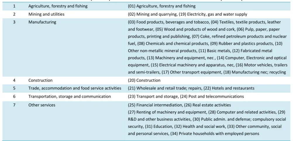
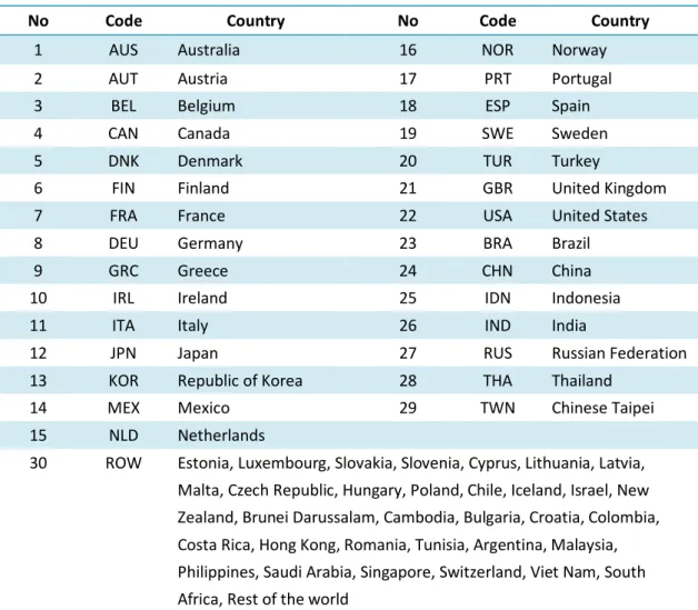
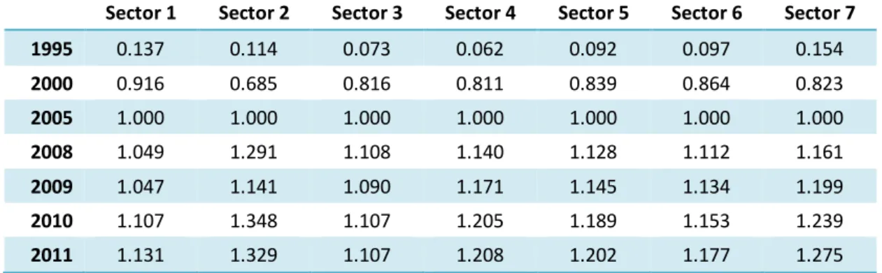
This paper employs OECD’s Intercountry Input-Output Tables 2015 edition and United Nations’ National Accounts in order to make international input-output tables in constant prices and local currencies. Since sector classifications differ between the two data sources, we reorganized sector classification as in Table 1. Regions are also aggregated as Table 2 shows. Following the steps described in the previous section, we computed price by sector and country. The computed prices for selected countries are presented in Table 3.
3.
The Model
3.1. The Theoretical Structure 3.1.1. Total Output
5 determined by the following equation:
����ℎ =� � ���
��ℎ� �
�=1 �
�=1
+� �����ℎ�
�
�=1
+� �����ℎ�
�
�=1
+� �����ℎ�
�
�=1
+� ����ℎ�
�
�=1
+� �����ℎ�
�
�=1
+� �����ℎ
�
�=1
+����ℎ
(4)
where ����ℎ is total output in sector i of country h in constant prices and currency h, �����ℎ� is intermediate goods delivered from sector i of country h to sector j of country k in constant prices and currency h, �����ℎ� is private consumption of country k delivered from sector i of country h denominated in constant prices and currency h, �����ℎ� is nonprofit institution serving household of country k delivered from sector i of country h in constant prices and currency h (exogenous), �����ℎ� is government consumption of country k delivered from sector i of country
h in constant prices and currency h (exogenous), ����ℎ� is fixed investment of country k delivered from sector i of country h in constant prices and currency h, �����ℎ� is inventories of country k delivered from sector i of country h in constant prices and currency h (exogenous), �����ℎ� is exports to the rest of the world in sector i of country h in constant prices and currency h (exogenous) and ����ℎ is statistical discrepancies in sector i of country h in constant prices and currency h (exogenous).
3.1.2. Firm Behavior
In this paper, we consider a case of monopoly. The producer in sector j of country k is assumed to have the following modified version of a generalized Ozaki cost function:1
����=� ��������������� �
�=1
+��������������
�
���exp�������
+���� ����������
�
����exp����� ��
(5)
where ���� is unit cost in sector j of country k denominate in the currency k, ����� is total output in sector j of country k in constant prices and currency k, ������ is price for intermediate goods in sector j of country k delivered from sector i in constant prices and currency k ������� = ∑�ℎ=1�����ℎ��, ��� is the wage rate in sector j of country k evaluated in current prices and
denominated in currency k, ���� is price of capital in sector j of country k denominated in currency k and � is time trend.
Applying the Shephard’s lemma yields the following demand for input factors:
������ =�
�������� (6)
6
���=���� ����������
�
exp������� (7)
����=���� ����������
�
exp����� �� (8)
where ��� is employment in sector j of country k and ���� is capital stock in sector j of country k denominated in currency k.
The allocation of intermediate input by sector into source countries is determined by the Armington’s (1969) approach as:
�����ℎ�=�����ℎ�������
��ℎ� � ���
������ (9)
where ��ℎ�=��ℎ����
�ℎ� �
��∗
�ℎ∗�
� � and ��ℎ is price in sector i of country h denominated in currency
h. Price for the Armington aggregate, ������, is expressed as:
������ =�������ℎ����
�
���ℎ��1−��
�
�
ℎ=1
�
1 1−���
(10)
Intermediate goods delivered from sector i of country h to sector j of country k in constant prices and currency h, �����ℎ�, is written as:
�����ℎ� =��� �� ℎ���ℎ
∗
��∗� (11)
3.1.3. Sectoral Price
Taking partial derivative of the cost function gives the following marginal cost:
����=� � �� ���� ��� � �=1 +������������������ �−1
���exp�� �����
+���� ���� ����������
�−1
����exp����� ��
(12)
where ���� is marginal cost in sector j of country k denominate in the currency k. Thus, the expression for sectoral price is written as:
���= ���
���−1���
� (13)
7
Slightly modifying the Philipps curve, we explain the sectoral wage rate by price deflator for private consumption and labor productivity as:
��� =�
�������,
�����
��� � (14)
where ���� is price deflator for private consumption in country k denominated in currency k.
3.1.5. Household Behavior
3.1.5.1. Private Consumption by Sector
Household of country k solves the following utility maximization problem:
max �����������
�
�
�=1
(15)
subject to
���=� ����
�������� �
�
(16)
where ������ is private consumption for goods i in country k in constant prices and currency k,
��� is household income of country k in current prices and currency k, and ����
�� price for
private consumption for goods i in country k denominated in currency k. As a result of this utility maximization problem, we obtain the following equation:
������= �� �
��������� (17)
3.1.5.2. Private Consumption by Sector and Country
Similar to the allocation of intermediate goods into source countries, we apply the Armington’s (1969) approach to allocation sectoral private consumption as:
�����ℎ�=���� ������
ℎ�����
��
��ℎ� � ���
(18)
8
������=������ℎ����
�
���ℎ��1−��
�
�
ℎ=1
�
1 1−���
(19)
3.1.5.3. Price for Private Consumption at the Macro Level
As one of the results of utility maximization, price for private consumption of country k denominated in currency k is formulated as:
�����=� ������� ��� � ��� � �=1 (20)
3.1.5.4. Household Income
Since the main source of household income is wages. Thus, household income is written as:
���=����� �
����� �
�=1
� (21)
3.1.6. Fixed Investment
Given capital stock explained by firm behavior, fixed investment is determined as follows:
����=������ �� �� �
�=1
� (22)
where ���� is fixed investment in country k in constant prices and currency k and ���� is depreciation in country k in constant prices and currency k (exogenous).
Fixed investment at the macro level is allocated into by using fixed coefficients as follows: based on Leontief. In detail, investment of sector i in country k, can be written as:
�����=�
�������� (23)
where ����� is fixed investment of sector i in country k in constant prices and currency k and ��� �� is the ratio of ����� to ����.
Allocation to source countries is determined by the Armington approach as:
����ℎ�=���������
ℎ����
��
��ℎ� � ���
(24)
9
�����=������ℎ����
�
���ℎ��1−��
�
�
ℎ=1
�
1 1−���
(25)
3.2. Estimation Results of Selected Variables
For parameter estimation, panel data method is employed. Since the unobservable individual effects are assumed to present country-specific or sector-specific factors, the fixed-effect model is applied. Data for the year 1995 is omitted since the euro is launched in 1999.
3.2.1. Employment by Sector
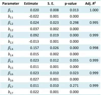
For estimation, we assume that parameters ���� and ���� are common among countries. Thus, by taking logarithms of equation (7), the estimation equation of employment by sector is expressed as:
ln��� =���� +���ln�����+���� (26)
Table 4 demonstrates the estimation results for the parameters ��� and ��� for all sectors. Although ��2 and ��7 are not statistically significant, the parameter ��� is all positive and less than the unity. This implies that economies of scale are found for labor demand in exception to the mining and utilities as well as other services sectors.
3.2.2. Sectoral Price
Table 5 illustrates estimation results of equation (13) for the agriculture, manufacturing and other services sectors. All estimated coefficients are greater than one and statistically significant. This indicates that substantial markups exist. Particularly, the markups in the other services sector are slightly greater than those in the agriculture and manufacturing sectors. We also note that coefficients exceed the unity and statistically significant for the rest of industrial sectors.
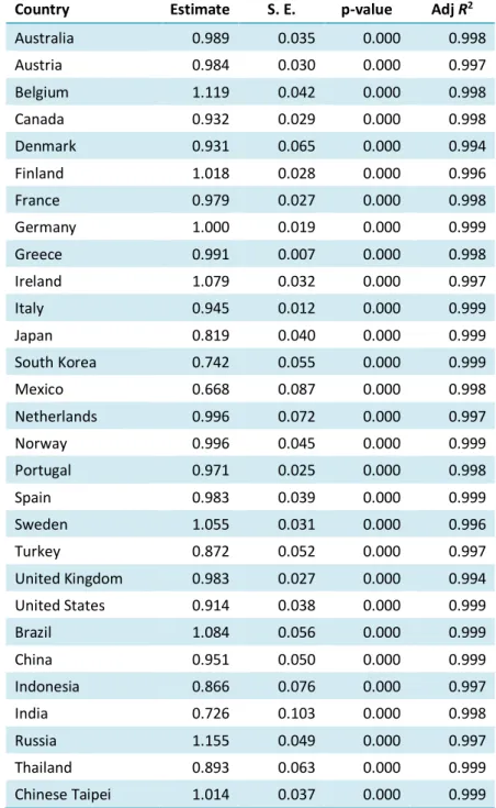
3.2.3. Private Consumption by Sector and Country
Taking logarithms of equation (18) gives the estimated equation of private consumption by sector and country as:
ln�����
ℎ�
������
=���ln���ℎ�+���ln�����
�
��ℎ�
(27)
10
Sweden, Brazil, Russia and Chinese Taipei are elastic (greater than the unity) whereas Japan, South Korea, Mexico, Turkey, Indonesia, India, Thailand are inelastic (less than 0.9).
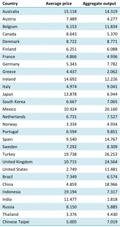
3.3. Results for the Final Test
In order to test model performance for the years 2000, 2005, 2008, 2009, 2010 and 2011, we compute the root mean square percentage errors (RMSPEs) of the weighted average of sectoral price and aggregate output. As Table 7 shows RMSPEs of the average price are greater than 10 percent for Australia, Ireland, Japan, Mexico, Turkey, the United Kingdom, Indonesia and India while we also found critical errors regarding aggregate output for Australia, Belgium, Ireland, Mexico, Spain, Turkey, the United Kingdom, the United States and China. These errors might result from estimation with the data set of mixture of developed and developing countries. Under the circumstance of data availability for econometric estimation, we can conclude that the model shows certain performance.
It is also worth noting that statistically insignificant parameters are employed for the construction of the global multi-sectoral model as long as the signs are correct. As for the Armington approach, the base-year fixed proportion is applied for the case of wrong sign. Approximately 34 percent, 32 percent and 61 percent of intermediates, private consumption, investment are explained by the fixed proportions, respectively.
4.
Application Example
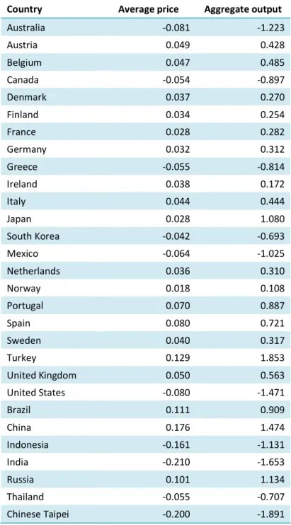
As an example of model applications, we examine the effects of 10 percent depreciation of the Japanese yen in 2005.
4.1. Macroeconomic Effects
Table 8 presents the effects on the average price and aggregate output. We found the negative impacts on the following countries: Australia, Canada, Greece, South Korea, Mexico, the United States, Indonesia, India, Thailand and Chinese Taipei. Among these countries, the negative effects on Indonesia, India and Chinese Taipei are slightly large. With respect to output, we also found that the effects on Australia and the United States are relatively large. By contrast, Turkey, Brazil and China have large positive impacts.
In absolute value, the maximum effect is 0.21 percent. Compare to the change in the Japanese yen (10 percent), the effects on price and output are small.
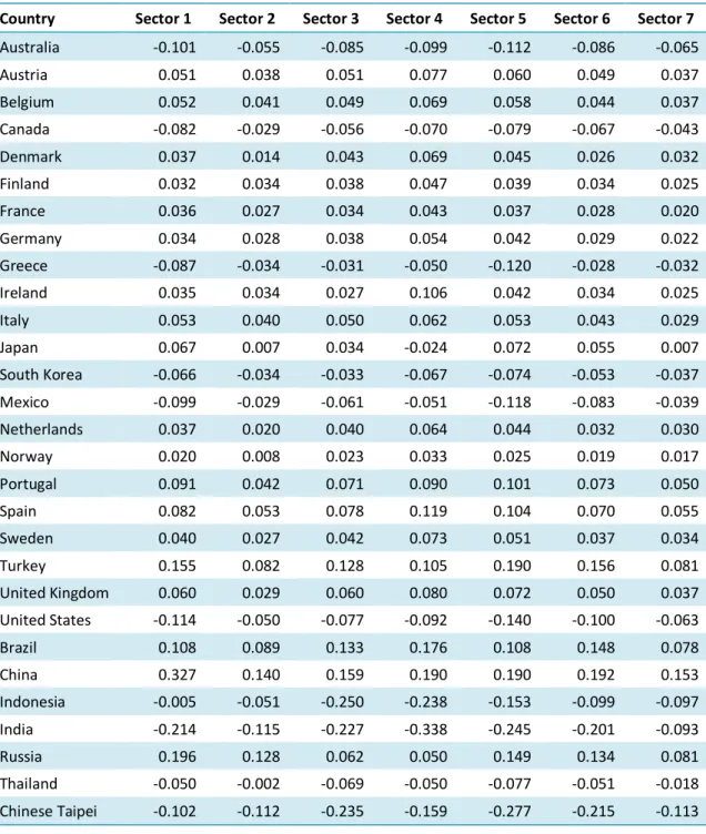
4.2. Sectoral Effects
Table 9 demonstrates the effects on sectoral price and output. Regarding Japan, price in the construction sector declines whereas those in the other sectors rise. Particularly, we found large positive effects in the agricultural sector, the trade sector and the transportation sectors. In contrast, output increases for all sectors in Japan.
11
sectors. As for sectoral price, we found the maximum positive impacts in all sectors of China whereas the maximum negative impacts are found in Indonesia (agriculture, mining and utilities, construction), India (manufacturing) and Chinese Taipei (trade, transportation and other services). Regarding output, Japan (manufacturing), Turkey (Mining and utilities, trade and transportation), China (agriculture and other services) and Russia (construction) have the greatest positive impacts within sectors while India (manufacturing and trade) and Chinese Taipei (agriculture, mining and utilities, construction, transportation and other services) face the largest negative impacts within sectors.
Among sectors, we found relatively large impacts on both price and output in the agricultural sector. By contrast, the impacts on output in the construction sector is quite limited. In total, the effects on output are far greater than those on price.
4.3. Discussion
By the depreciation of the yen, price of the Japanese goods denominated in U.S. dollars falls while Japan faces price rise in imported goods denominated in the Japanese yen. The former increases exports of the while the latter decreases imports. With these effects, Japan’s price and output increase. Particularly, domestic price change of Japan is only 0.03 percent while the exchange rate changes 10 percent. Thus, Japan’s relative price is greatly improved. This results in an output increase.
For the other countries than Japan, Japan’s price decrease in U.S. dollars can yield two outcomes. First, price in both U.S. dollars and local currencies falls. This could result in increases of demand and price. Second, Japan’s relative price improves. This could be a cause of decreases in export demand and price. Although further analysis is required, it might be tentatively concluded that the impacts through the first route are greater than those through the second one in countries with positive effects (the reverse occurs to countries with negative effects).
5.
Conclusions
In this paper, we constructed international input-output tables evaluated in constant prices and denominated in local currencies. We also developed the theoretical structure of a local-currency-based multi-country multi-sectoral model with economies of scale and monopoly. Similar to widely used CGE models, the model has micro foundations; however, most parameters of the model are econometrically estimated.
12
References
Almon, Clopper. 1991. “The INFORUM Approach to Interindustry Modeling.” Economic Systems
Research 3, no. 1: 1-7.
Armington, Paul. S. 1969. “A Theory of Demand for Products Distinguished by Place of Production,” IMF Staff Papers 16, no. 1: 159-178.
Deardorff, Alan V. and Robert M. Stern. 1986. The Michigan Model of World Production and Trade. Cambridge, Mass.: MIT Press.
Dietzenbacher, Erik and Alex R. Hoen. 1998. “Deflation of Input-Output Tables from the User’s Point of View: A Heuristic Approach.” Review of Income and Wealth 44, no.1: 111-122.
Fair, Ray C. 1994. Testing Macroeconometric Models. Cambridge, Mass.: Harvard University Press.
Hertel, Thomas W., ed. 1997. Global Trade Analysis: Modeling and Applications. Cambridge: Cambridge University Press.
Hoen, Alex R. 2002. An Input-Output Analysis of European Integration. Amsterdam: Elsevier.
Klein, Lawrence R. 1950. Economic Fluctuations in the United States 1921-1941. New York: John Wiley and Sons.
Kosaka, Hiroyuki. 1994. Gurōbaru shisutemu no moderu bunseki [Model analysis on global
system]. Tokyo: Yuhikaku.
McKibbin, Warwick J. and Peter J. Wilcoxen. 1999. “The Theoretical and Empirical Structure of the G-Cubed Model.” Economic Modelling 16, no.1: 123-148.
Nakamura, Shinichiro. 1990. “A Nonhomothetic Generalized Leontief Cost Function Based on Pooled Data.” Review of Economics and Statistics 72, no. 4: 649-656.
Pesenti, Paolo. 2008. “The Global Economy Model: Theoretical Framework.” IMF Staff Papers 44, no. 2: 243-284.
Taylor, John B. 1993. Macroeconomic Policy in a World Economy: From Econometric Design to
13
Torii, Yasuhiko, Seung-Jin Shim, and Yutaka Akiyama. 1989. “Effects of Tariff Reductions on Trade in the Asia-Pacific Region.” In Frontiers in Input-Output Analysis, eds. Ronald E. Millar, Karen R. Polenske and Adam Z. Rose. New York: Oxford University Press. pp. 165-179.
Uno, Kimio, ed. 2002. Economy-Energy-Environment Simulation: Beyond the Kyoto Protocol. Dordrecht: Kluwer Academic Publishers.
Yano, Takashi and Hiroyuki Kosaka. 2003. “Trade Patterns and Exchange Rate Regimes: Testing the Asian Currency Basket Using an International Input-Output System.” Developing
Economies 41, no. 1: 3-36.
Yano, Takashi and Hiroyuki Kosaka. 2015. “Development of a Multi-Country Multi-Sectoral Model in International Dollars.” In New Solutions in Legal Informatics, Economic Sciences
and Mathematics, eds. Munenori Kitahara and Kazuaki Okamura. Fukuoka: Kyushu
14
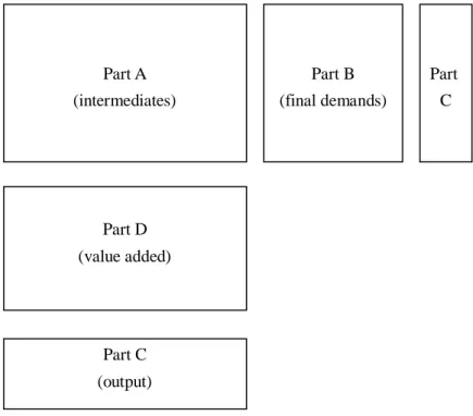
Figure 1: A Structure of International Input-Output Tables
Part A (intermediates)
Part B (final demands)
Part C
Part D (value added)
15
Table 1: Sector Classification
New Sector Classification (7 sectors) OECD ICIO Classification (34 sectors)
1 Agriculture, forestry and fishing (01) Agriculture, forestry and fishing
2 Mining and utilities (02) Mining and quarrying, (19) Electricity, gas and water supply
3 Manufacturing (03) Food products, beverages and tobacco, (04) Textiles, textile products, leather
and footwear, (05) Wood and products of wood and cork, (06) Pulp, paper, paper
products, printing and publishing, (07) Coke, refined petroleum products and nuclear
fuel, (08) Chemicals and chemical products, (09) Rubber and plastics products, (10)
Other non-metallic mineral products, (11) Basic metals, (12) Fabricated metal
products, (13) Machinery and equipment, nec , (14) Computer, Electronic and optical
equipment, (15) Electrical machinery and apparatus, nec, (16) Motor vehicles, trailers
and semi-trailers, (17) Other transport equipment, (18) Manufacturing nec; recycling
4 Construction (20) Construction
5 Trade, accommodation and food service activities (21) Wholesale and retail trade; repairs, (22) Hotels and restaurants
6 Transportation, storage and communication (23) Transport and storage, (24) Post and telecommunications
7 Other services (25) Financial intermediation, (26) Real estate activities
(27) Renting of machinery and equipment, (28) Computer and related activities, (29)
R&D and other business activities, (30) Public admin. and defense; compulsory social
security, (31) Education, (32) Health and social work, (33) Other community, social
16
Table 2: Regional Classification
No Code Country No Code Country
1 AUS Australia 16 NOR Norway
2 AUT Austria 17 PRT Portugal
3 BEL Belgium 18 ESP Spain
4 CAN Canada 19 SWE Sweden
5 DNK Denmark 20 TUR Turkey
6 FIN Finland 21 GBR United Kingdom
7 FRA France 22 USA United States
8 DEU Germany 23 BRA Brazil
9 GRC Greece 24 CHN China
10 IRL Ireland 25 IDN Indonesia
11 ITA Italy 26 IND India
12 JPN Japan 27 RUS Russian Federation
13 KOR Republic of Korea 28 THA Thailand
14 MEX Mexico 29 TWN Chinese Taipei
15 NLD Netherlands
30 ROW Estonia, Luxembourg, Slovakia, Slovenia, Cyprus, Lithuania, Latvia,
Malta, Czech Republic, Hungary, Poland, Chile, Iceland, Israel, New
Zealand, Brunei Darussalam, Cambodia, Bulgaria, Croatia, Colombia,
Costa Rica, Hong Kong, Romania, Tunisia, Argentina, Malaysia,
Philippines, Saudi Arabia, Singapore, Switzerland, Viet Nam, South
17
Table 3: Selected Countries’ Computed Sectoral Prices
Australia
Sector 1 Sector 2 Sector 3 Sector 4 Sector 5 Sector 6 Sector 7
1995 0.137 0.114 0.073 0.062 0.092 0.097 0.154
2000 0.916 0.685 0.816 0.811 0.839 0.864 0.823
2005 1.000 1.000 1.000 1.000 1.000 1.000 1.000
2008 1.049 1.291 1.108 1.140 1.128 1.112 1.161
2009 1.047 1.141 1.090 1.171 1.145 1.134 1.199
2010 1.107 1.348 1.107 1.205 1.189 1.153 1.239
2011 1.131 1.329 1.107 1.208 1.202 1.177 1.275
France
Sector 1 Sector 2 Sector 3 Sector 4 Sector 5 Sector 6 Sector 7
1995 0.176 0.206 0.102 0.131 0.235 0.240 0.309
2000 0.873 0.842 0.814 0.787 0.844 0.865 0.849
2005 1.000 1.000 1.000 1.000 1.000 1.000 1.000
2008 1.015 1.049 1.049 1.149 1.054 1.028 1.087
2009 0.905 1.084 1.031 1.156 1.070 1.041 1.086
2010 1.041 1.130 1.054 1.183 1.076 1.034 1.106
2011 1.060 1.201 1.069 1.219 1.076 1.018 1.116
Germany
Sector 1 Sector 2 Sector 3 Sector 4 Sector 5 Sector 6 Sector 7
1995 0.070 0.110 0.046 0.060 0.126 0.095 0.195
2000 0.845 0.790 0.732 0.814 0.815 0.691 0.854
2005 1.000 1.000 1.000 1.000 1.000 1.000 1.000
2008 0.978 1.188 1.023 1.082 1.009 0.967 1.024
2009 0.894 1.103 1.037 1.100 1.042 0.968 1.042
2010 1.047 1.149 1.059 1.127 1.056 0.983 1.061
18
Japan
Sector 1 Sector 2 Sector 3 Sector 4 Sector 5 Sector 6 Sector 7
1995 0.289 0.409 0.194 0.230 0.372 0.394 0.417
2000 1.023 1.130 1.057 1.020 1.027 1.048 1.017
2005 1.000 1.000 1.000 1.000 1.000 1.000 1.000
2008 0.908 0.924 0.967 1.020 1.026 0.971 0.982
2009 0.920 1.054 0.948 0.997 1.000 0.974 0.974
2010 0.937 0.996 0.923 0.985 0.989 0.957 0.963
2011 0.902 0.955 0.901 0.978 0.986 0.942 0.953
Mexico
Sector 1 Sector 2 Sector 3 Sector 4 Sector 5 Sector 6 Sector 7
1995 0.151 0.138 0.059 0.074 0.169 0.152 0.202
2000 0.773 0.612 0.703 0.689 0.730 0.794 0.693
2005 1.000 1.000 1.000 1.000 1.000 1.000 1.000
2008 1.211 1.339 1.218 1.197 1.175 1.137 1.150
2009 1.259 1.248 1.293 1.245 1.241 1.185 1.195
2010 1.320 1.360 1.336 1.289 1.271 1.239 1.223
2011 1.451 1.583 1.413 1.367 1.331 1.259 1.267
Turkey
Sector 1 Sector 2 Sector 3 Sector 4 Sector 5 Sector 6 Sector 7
1995 0.003 0.003 0.002 0.001 0.004 0.002 0.003
2000 0.204 0.244 0.223 0.224 0.267 0.250 0.295
2005 1.000 1.000 1.000 1.000 1.000 1.000 1.000
2008 1.231 1.412 1.276 1.320 1.318 1.306 1.355
2009 1.294 1.556 1.324 1.340 1.354 1.345 1.446
2010 1.449 1.607 1.377 1.399 1.399 1.387 1.495
2011 1.557 1.754 1.563 1.591 1.576 1.529 1.566
United States
Sector 1 Sector 2 Sector 3 Sector 4 Sector 5 Sector 6 Sector 7
1995 0.133 0.186 0.090 0.088 0.210 0.202 0.226
2000 0.761 0.622 0.785 0.705 0.824 0.770 0.797
2005 1.000 1.000 1.000 1.000 1.000 1.000 1.000
2008 1.177 1.236 1.091 1.138 1.093 1.051 1.094
2009 1.040 1.080 1.069 1.132 1.122 1.054 1.099
2010 1.129 1.164 1.104 1.145 1.140 1.065 1.120
19
Brazil
Sector 1 Sector 2 Sector 3 Sector 4 Sector 5 Sector 6 Sector 7
1995 0.065 0.046 0.027 0.035 0.131 0.043 0.093
2000 0.633 0.559 0.584 0.612 0.600 0.619 0.659
2005 1.000 1.000 1.000 1.000 1.000 1.000 1.000
2008 1.193 1.205 1.168 1.170 1.296 1.236 1.213
2009 1.302 1.124 1.260 1.359 1.456 1.330 1.304
2010 1.312 1.328 1.300 1.496 1.531 1.407 1.399
2011 1.438 1.524 1.378 1.576 1.720 1.631 1.462
China
Sector 1 Sector 2 Sector 3 Sector 4 Sector 5 Sector 6 Sector 7
1995 0.262 0.153 0.100 0.140 0.231 0.227 0.234
2000 0.813 0.927 0.819 0.839 0.857 0.871 0.785
2005 1.000 1.000 1.000 1.000 1.000 1.000 1.000
2008 1.248 1.246 1.129 1.153 1.142 1.149 1.153
2009 1.237 1.185 1.094 1.132 1.127 1.119 1.164
2010 1.347 1.308 1.166 1.206 1.204 1.175 1.245
2011 1.483 1.417 1.235 1.292 1.294 1.249 1.343
India
Sector 1 Sector 2 Sector 3 Sector 4 Sector 5 Sector 6 Sector 7
1995 0.273 0.148 0.088 0.111 0.287 0.148 0.256
2000 0.799 0.733 0.774 0.732 0.774 0.864 0.781
2005 1.000 1.000 1.000 1.000 1.000 1.000 1.000
2008 1.319 1.207 1.211 1.247 1.221 1.132 1.218
2009 1.484 1.322 1.266 1.304 1.282 1.151 1.302
2010 1.651 1.454 1.356 1.399 1.408 1.183 1.424
20
Table 4: Estimation Results of Employment by Sector
Parameter Estimate S. E. p-value Adj. R2
��1 0.020 0.008 0.013 1.000
��1 -0.022 0.001 0.000
��2 0.024 0.023 0.298 0.995
��2 0.037 0.002 0.000
��3 0.092 0.019 0.000 0.999
��3 -0.013 0.001 0.000
��4 0.157 0.026 0.000 0.998
��4 0.015 0.002 0.000
��5 0.023 0.012 0.055 0.999
��5 0.011 0.001 0.000
��6 0.023 0.010 0.023 0.999
��6 0.027 0.001 0.000
��7 0.011 0.010 0.271 0.999
��7 0.022 0.001 0.000
21
Table 5: Estimation Results of Sectoral Price
Agricultural sector
Country Estimate S. E. p-value
Australia 1.094 0.014 0.000
Austria 1.045 0.011 0.000
Belgium 1.005 0.012 0.000
Canada 1.177 0.019 0.000
Denmark 1.151 0.017 0.000
Finland 1.110 0.011 0.000
France 1.114 0.005 0.000
Germany 1.161 0.030 0.000
Greece 1.115 0.024 0.000
Ireland 1.073 0.028 0.000
Italy 1.098 0.012 0.000
Japan 1.163 0.021 0.000
South Korea 1.044 0.007 0.000
Mexico 1.065 0.004 0.000
Netherlands 1.087 0.011 0.000
Norway 1.092 0.014 0.000
Portugal 1.109 0.009 0.000
Spain 1.069 0.007 0.000
Sweden 1.188 0.013 0.000
Turkey 2.125 0.024 0.000
United Kingdom 1.196 0.017 0.000
United States 1.094 0.012 0.000
Brazil 1.211 0.013 0.000
China 2.129 0.074 0.000
Indonesia 1.560 0.029 0.000
India 1.067 0.002 0.000
Russia 1.539 0.025 0.000
Thailand 1.069 0.016 0.000
Chinese Taipei 1.703 0.016 0.000
Adj R2 0.994
22 Manufacturing sector
Country Estimate S. E. p-value
Australia 1.253 0.006 0.000
Austria 1.279 0.016 0.000
Belgium 1.150 0.013 0.000
Canada 1.237 0.004 0.000
Denmark 1.241 0.010 0.000
Finland 1.151 0.015 0.000
France 1.214 0.010 0.000
Germany 1.285 0.021 0.000
Greece 1.506 0.037 0.000
Ireland 1.093 0.013 0.000
Italy 1.189 0.011 0.000
Japan 1.228 0.009 0.000
South Korea 1.171 0.005 0.000
Mexico 1.070 0.007 0.000
Netherlands 1.170 0.013 0.000
Norway 1.210 0.013 0.000
Portugal 1.233 0.014 0.000
Spain 1.223 0.011 0.000
Sweden 1.142 0.017 0.000
Turkey 1.134 0.006 0.000
United Kingdom 1.243 0.019 0.000
United States 1.189 0.021 0.000
Brazil 1.206 0.010 0.000
China 1.088 0.002 0.000
Indonesia 1.175 0.006 0.000
India 1.170 0.005 0.000
Russia 1.193 0.006 0.000
Thailand 1.177 0.004 0.000
Chinese Taipei 1.227 0.012 0.000
Adj R2 0.994
23 Other services sector
Country Estimate S. E. p-value
Australia 1.498 0.006 0.000
Austria 1.545 0.012 0.000
Belgium 1.511 0.013 0.000
Canada 1.591 0.008 0.000
Denmark 1.709 0.009 0.000
Finland 1.588 0.014 0.000
France 1.565 0.005 0.000
Germany 1.502 0.014 0.000
Greece 1.518 0.024 0.000
Ireland 1.397 0.021 0.000
Italy 1.393 0.008 0.000
Japan 1.489 0.006 0.000
South Korea 1.510 0.011 0.000
Mexico 1.448 0.006 0.000
Netherlands 1.565 0.009 0.000
Norway 1.634 0.019 0.000
Portugal 1.580 0.016 0.000
Spain 1.608 0.017 0.000
Sweden 1.494 0.009 0.000
Turkey 1.268 0.011 0.000
United Kingdom 1.486 0.022 0.000
United States 1.526 0.007 0.000
Brazil 1.644 0.027 0.000
China 1.272 0.009 0.000
Indonesia 1.587 0.020 0.000
India 1.490 0.022 0.000
Russia 1.678 0.014 0.000
Thailand 1.500 0.020 0.000
Chinese Taipei 1.637 0.012 0.000
Adj R2 0.989
24
Table 6: Estimation Results of Private Consumption by Sector and Country (Manufacturing)
Country Estimate S. E. p-value Adj R2
Australia 0.989 0.035 0.000 0.998
Austria 0.984 0.030 0.000 0.997
Belgium 1.119 0.042 0.000 0.998
Canada 0.932 0.029 0.000 0.998
Denmark 0.931 0.065 0.000 0.994
Finland 1.018 0.028 0.000 0.996
France 0.979 0.027 0.000 0.998
Germany 1.000 0.019 0.000 0.999
Greece 0.991 0.007 0.000 0.998
Ireland 1.079 0.032 0.000 0.997
Italy 0.945 0.012 0.000 0.999
Japan 0.819 0.040 0.000 0.999
South Korea 0.742 0.055 0.000 0.999
Mexico 0.668 0.087 0.000 0.998
Netherlands 0.996 0.072 0.000 0.997
Norway 0.996 0.045 0.000 0.999
Portugal 0.971 0.025 0.000 0.998
Spain 0.983 0.039 0.000 0.999
Sweden 1.055 0.031 0.000 0.996
Turkey 0.872 0.052 0.000 0.997
United Kingdom 0.983 0.027 0.000 0.994
United States 0.914 0.038 0.000 0.999
Brazil 1.084 0.056 0.000 0.999
China 0.951 0.050 0.000 0.999
Indonesia 0.866 0.076 0.000 0.997
India 0.726 0.103 0.000 0.998
Russia 1.155 0.049 0.000 0.997
Thailand 0.893 0.063 0.000 0.999
Chinese Taipei 1.014 0.037 0.000 0.999
25
Table 7: Final Test Results (Root Mean Square Percentage Errors)
Country Average price Aggregate output
Australia 15.118 14.319
Austria 7.489 4.277
Belgium 6.153 11.834
Canada 8.643 5.370
Denmark 8.722 8.771
Finland 6.251 6.088
France 4.866 4.936
Germany 5.343 7.782
Greece 4.437 2.062
Ireland 14.692 12.226
Italy 4.974 9.041
Japan 13.878 6.944
South Korea 6.667 7.065
Mexico 10.924 20.160
Netherlands 6.731 7.527
Norway 3.334 4.934
Portugal 6.594 9.851
Spain 9.540 14.767
Sweden 7.292 8.309
Turkey 19.738 26.253
United Kingdom 10.715 24.564
United States 2.749 11.481
Brazil 7.349 6.574
China 4.859 18.966
Indonesia 19.194 7.317
India 11.477 1.818
Russia 8.150 5.885
Thailand 3.376 4.430
26
Table 8: Percent Deviations of Average Price and Aggregate Output from the Baseline
Country Average price Aggregate output
Australia -0.081 -1.223
Austria 0.049 0.428
Belgium 0.047 0.485
Canada -0.054 -0.897
Denmark 0.037 0.270
Finland 0.034 0.254
France 0.028 0.282
Germany 0.032 0.312
Greece -0.055 -0.814
Ireland 0.038 0.172
Italy 0.044 0.444
Japan 0.028 1.080
South Korea -0.042 -0.693
Mexico -0.064 -1.025
Netherlands 0.036 0.310
Norway 0.018 0.108
Portugal 0.070 0.887
Spain 0.080 0.721
Sweden 0.040 0.317
Turkey 0.129 1.853
United Kingdom 0.050 0.563
United States -0.080 -1.471
Brazil 0.111 0.909
China 0.176 1.474
Indonesia -0.161 -1.131
India -0.210 -1.653
Russia 0.101 1.134
Thailand -0.055 -0.707
27
Table 9: Percent Deviations of Sectoral Price and Output from the Baseline
Sectoral price
Country Sector 1 Sector 2 Sector 3 Sector 4 Sector 5 Sector 6 Sector 7
Australia -0.101 -0.055 -0.085 -0.099 -0.112 -0.086 -0.065
Austria 0.051 0.038 0.051 0.077 0.060 0.049 0.037
Belgium 0.052 0.041 0.049 0.069 0.058 0.044 0.037
Canada -0.082 -0.029 -0.056 -0.070 -0.079 -0.067 -0.043
Denmark 0.037 0.014 0.043 0.069 0.045 0.026 0.032
Finland 0.032 0.034 0.038 0.047 0.039 0.034 0.025
France 0.036 0.027 0.034 0.043 0.037 0.028 0.020
Germany 0.034 0.028 0.038 0.054 0.042 0.029 0.022
Greece -0.087 -0.034 -0.031 -0.050 -0.120 -0.028 -0.032
Ireland 0.035 0.034 0.027 0.106 0.042 0.034 0.025
Italy 0.053 0.040 0.050 0.062 0.053 0.043 0.029
Japan 0.067 0.007 0.034 -0.024 0.072 0.055 0.007
South Korea -0.066 -0.034 -0.033 -0.067 -0.074 -0.053 -0.037
Mexico -0.099 -0.029 -0.061 -0.051 -0.118 -0.083 -0.039
Netherlands 0.037 0.020 0.040 0.064 0.044 0.032 0.030
Norway 0.020 0.008 0.023 0.033 0.025 0.019 0.017
Portugal 0.091 0.042 0.071 0.090 0.101 0.073 0.050
Spain 0.082 0.053 0.078 0.119 0.104 0.070 0.055
Sweden 0.040 0.027 0.042 0.073 0.051 0.037 0.034
Turkey 0.155 0.082 0.128 0.105 0.190 0.156 0.081
United Kingdom 0.060 0.029 0.060 0.080 0.072 0.050 0.037
United States -0.114 -0.050 -0.077 -0.092 -0.140 -0.100 -0.063
Brazil 0.108 0.089 0.133 0.176 0.108 0.148 0.078
China 0.327 0.140 0.159 0.190 0.190 0.192 0.153
Indonesia -0.005 -0.051 -0.250 -0.238 -0.153 -0.099 -0.097
India -0.214 -0.115 -0.227 -0.338 -0.245 -0.201 -0.093
Russia 0.196 0.128 0.062 0.050 0.149 0.134 0.081
Thailand -0.050 -0.002 -0.069 -0.050 -0.077 -0.051 -0.018
28 Sectoral output
Country Sector 1 Sector 2 Sector 3 Sector 4 Sector 5 Sector 6 Sector 7
Australia -1.305 -1.912 -1.256 -0.318 -1.547 -1.285 -1.199
Austria 0.576 0.601 0.308 0.179 0.547 0.606 0.453
Belgium 0.721 0.708 0.492 0.150 0.619 0.458 0.482
Canada -1.230 -1.188 -1.108 -0.121 -1.092 -0.978 -0.745
Denmark 0.459 0.457 0.242 0.076 0.391 0.033 0.326
Finland 0.331 0.316 0.192 0.062 0.368 0.389 0.281
France 0.448 0.462 0.278 0.062 0.383 0.338 0.257
Germany 0.402 0.452 0.249 0.102 0.431 0.367 0.339
Greece -1.042 -1.114 -0.798 -0.130 -1.204 -0.325 -0.832
Ireland 0.455 0.466 0.013 0.029 0.362 0.589 0.206
Italy 0.617 0.617 0.395 0.133 0.571 0.530 0.434
Japan 1.211 0.850 2.021 0.131 1.229 1.303 0.271
South Korea -0.936 -0.905 -0.672 -0.055 -0.865 -0.962 -0.745
Mexico -1.233 -1.045 -1.176 -0.018 -1.174 -1.296 -0.947
Netherlands 0.444 0.451 0.384 0.080 0.414 0.274 0.249
Norway 0.134 0.210 0.069 0.036 0.160 0.064 0.094
Portugal 1.252 1.233 0.887 0.181 1.240 1.001 0.798
Spain 0.997 0.997 0.749 0.215 1.086 0.773 0.648
Sweden 0.466 0.578 0.226 0.136 0.406 0.390 0.348
Turkey 2.499 2.023 1.819 0.154 2.004 2.244 1.707
United Kingdom 0.891 0.711 0.505 0.237 0.918 0.734 0.471
United States -1.641 -1.677 -1.456 -0.294 -1.767 -1.671 -1.467
Brazil 1.102 0.913 0.927 0.207 1.188 1.124 0.850
China 3.103 1.482 1.136 0.118 1.519 2.036 2.459
Indonesia -1.383 -1.964 -1.101 -0.116 -1.354 -1.397 -0.977
India -2.693 -1.591 -1.536 -0.318 -2.154 -2.072 -1.535
Russia 2.497 0.587 1.066 0.323 1.437 1.374 1.155
Thailand -0.727 -0.639 -0.820 -0.199 -0.796 -0.804 -0.408