Abstract
Evidence shows that important age and cohort effects exist in at-home consumption of most food products in present-day Japan. Individual consumption of rice, fish, meat and vegetables by age over the last three decades from 1980 to 2013 was derived from the
Family Income and Expenditure Survey classified by age groups of household head.
Aug-mented cohort models decomposed cohort tables into age, cohort and period effects along with demand elasticities of prices and income. Age and cohort effects thus determined were synthesized to predict consumption by age to 2015 and 2020, on the assumption that the economic conditions would stay the same as in 2009−11. These predictions by age, when combined with the projected population age structure, can be aggregated into total at -home consumption.
JEL 区分:C53, D03, D12
keywords:consumption by age, rice, fish, meat, vegetables, augmented cohort model
Acknowledgements
The authors are grateful to John Dyck of the U.S. Department of Agriculture, Economic Research Service, for valuable comments and suggestions on the earlier drafts and for thorough editing ; to Erica Mori for helpful graphical design ; and, last but not least, to Senshu University for providing a comfortable research environment.
*Professor Emeritus, Senshu University
**Professor of Statistics (retired), Tokyo Metropolitan University. ***Formerly at Nippon Reserch Center, Inc.
Augmented Cohort Analysis
―A Practical Way to Predict Future At-home
Consumption of Selected Food Products
Hiroshi Mori
*, Yoshiharu Saegusa
**1. Introduction
Food consumption varies by age. As one ages, physically and socially, consumption changes in quantity and in variety as well. When and/or where the population age structure is not stable, it is necessary to take the age factor into consideration in analyzing and projecting changes in food con-sumption. Age has long been incorporated in forecasting future food consumption in the United States, in particular (Price, 1970, 1979 ; Buse and Salathe, 1978 ; Salathe, 1979 ; Blaylock and Smallwood, 1986 ; Southard, 1987 ; Lin et al., 2003 ; Blisard et al., 2003 ; etc.).
Age is not just a matter of physical aging. Schrimper raised the issue in comments on Salathe’s presentation, “The effects of changes in population characteristics on U.S. food consumption” at the American Agricultural Economics Association meeting, 1979 : “Are variations in eating habits of older people relative to younger segments of the population the results of physiological differences, different economic circumstances, or are food habits partly a product of different generations of in-fluences? How much of the differences associated with age in any given cross-section are the re-sults of economic influences or partly cohort effects as compared to pure age effects? In other words, is it reasonable to expect all generations to follow the same transformation of eating habits over the life cycle, ceteris paribus?” (Schrimper, 1979, p. 1059).
Stewart et al. state, “since Schrimper (1979) first raised the possibility that cohort effects exist and shape trends in food consumption, much empirical research has followed” (Stewart, Dong, and Carlson, 2013, pp.7−9). In fact, however, after nearly three decades, such studies are few in num-ber : the case studies of fresh fruit and fish consumption in Japan by Mori et al. (2006) and Mori and Saegusa (2010), respectively and one analysis of expenditures on fresh vegetables in the United States by Stewart and Blisard (2008). Even after the turn of the century, projections of food con-sumption/expenditures by USDA-ERS are still based on ”the implicit assumptions that as any indi-vidual moves from one demographic group to another, his/her preferences immediately take on the characteristics of the new group. For example, younger age groups will assume the eating habits of older age groups as they age” (Lin et al., 2003, pp.13−14) ; “second, as their demographic circum-stances change, consumers are assumed to acquire the expenditure patterns of individuals already observed in those circumstances” (Blisard, Variyam, and Cromartie 2003, p.20). These assumptions are in line with the axiom of traditional microeconomics that “tastes neither change capriciously nor differ importantly between people.” Based on this viewpoint, “the economist continues to search for differences in prices and incomes to explain any differences or changes in behavior” (Stigler and Becker, 1977, p. 76 ; Chalfant and Alston, 1988).
(Huang and Bouis, 2001, p.68). The data reveal more information about consumption change when demographic factors are explicitly included in the analysis.
The Japanese Government Bureau of Statistics conducts diary-type expenditure surveys, the
Fam-ily Income and Expenditure Survey (FIES), of approximately 8,000 households across the country
every month and every year. Starting 1979, the FIES annual report publishes expenditures, quanti-ties and purchase prices of major goods and services, classified by the age groups of household heads (HH). This analysis first derives consumption by individual members of households by age by means of the Tanaka, Mori, and Inaba model (TMI) (Tanaka, Mori, and Inaba, 2004). Cohort ta-bles are constructed, covering 12 age groups from 15−19 years old to 70−74 years old for 34 years from 1980 to 2013. Three age groups under 15 are not used because of likely unstable estimates and the oldest, 75+, is excluded because this group contains more than one birth cohort in the cell every year. The general cohort table of an individual commodity is decomposed into age/cohort/ period (A/P/C) effects by the conventional Bayesian cohort model first and then by the “Bayesian augmented cohort model” along with elasticities of prices and incomes, and trend, if found not neg-ligible (Saegusa and Mori, 2012 ; Mori and Saegusa, 2013). Age, cohort and period effects thus de-termined are then synthesized to project individual consumption by age to the specific years, 2015 and 2020. Aggregate national consumption can then be calculated mechanically, using age struc-tures by 5- year bracket predicted by the Ministry of Health and Labor.
2. Visual Sketches of Household Consumption by Age
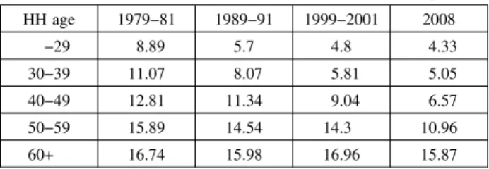
Table 1 provides per capita household consumption of fresh fish classified by HH age groups over the 30 year period from 1980 (Mori and Saegusa, 2010). Distinct age effects in household con-sumption of fish in present day Japan are apparent. Those in their 20s in 1980 belong to the cohort born in the 1950s and those in their 20s in 1990 and 2000 are cohorts born in the 1960s and the 1970s, respectively, and so on. The cohort born in the 1950s consumed, on average, 8.89kg in 1980, 8.07kg in 1990, 9.04kg in 2000 and 10.96kg in 2008, as they aged from their 20s to their 30s, their 40s and their 50s, respectively.
When following per capita consumption diagonally in the table, one notices that those belonging
Table 1 Changes in per capita At-home Consumption of
Fresh Fish by HH age Groups, 1980-2008
(kg/person) HH age 1979−81 1989−91 1999−2001 2008 −29 8.89 5.7 4.8 4.33 30−39 11.07 8.07 5.81 5.05 40−49 12.81 11.34 9.04 6.57 50−59 15.89 14.54 14.3 10.96 60+ 16.74 15.98 16.96 15.87
to the same cohort have kept their consumption of fish roughly at the same level, or slightly in-creased it as they aged over the period in question, implying that observed differences between age groups at any period might partially represent differences in cohort effects. When following per cap-ita consumption horizontally over the survey period, the younger groups in their 20s to 40s de-creased their consumption drastically, whereas the oldest age group above 60 years old did not change their consumption of fish conspicuously. No one can tell exactly how much of these differ-ences can be attributed to likely differdiffer-ences in period effects and those in age and cohort effects. Mathematically, i, as age, t, as period, and k, as cohort (the birth year) are lineally dependent on each other, i.e., t = i + k. This causes difficulties in identifying three separate effects of age, pe-riod and cohort in statistical cohort analysis either for epidemiology or social science (Glenn, 1977 ; Rodgers, 1982 ; Holford, 1983, 1991 ; Mason and Fienberg, 1985 ; Nakamura, 1982, 1986 ; Tabgo and Kurihara, 1987 ; Shahper and Li, 1999 ; Yang et al., 2008 ; Fu, 2008 ; etc.). Based on our own research experience of Japanese food consumption analyses in the past 15 years, we are inclined to presume that the Bayesian approach developed by Nakamura on the intuitively natural assumption of “gradual changes between successive parameters” might represent a fair approximation of changes in consumption of most food products in Japan from the age perspective (Mori et al., 2001 ; Tanaka et al., 2007 ; Mori, Saegusa, and Kawaguchi, 2008 ; Mori, 2014 ; etc.).
3. Data
Per capita consumption data in Table 1, used for visual explanation in the preceding section, are quantities of household annual fish consumption simply divided by the number of persons contained in the household in question. The FIES annual reports, which publish household consumption by HH age groups, do not cover single-person households. In 1980, for example, approximately 8,000 households surveyed averaged 3.82 persons in size and those, where HHs were 30−34 years old, for example, averaged 3.93 persons in size. It is expected that nearly 2 persons, husband and wife, in this household were in their early 30s and the remaining 2 persons were young children under 10 years of age. Dividing the household consumption by 3.93 to derive likely per capita consumption by those in their early 30s could be somewhat misleading, except for milk, for example, which small children consume nearly as much as their parents. The age compositions of households classified by HH age groups need to be explicitly incorporated in deriving per capita consumption by age of individual members of households from household data classified by HH age groups, such as those published in the FIES annual reports.
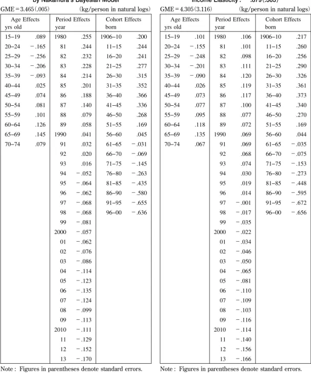
year (Tables 2, 3, 4 and 5). Cohort tables comprising 12 age groups from 15−19 years old to 70−74 years old and 34 years from 1980 to 2013 were decomposed into age, period and cohort effects by means of the conventional Bayesian model in kg/person in natural logs (Tables 6A, 7A, 8A and 9A). The period effects in the middle column are considered to represent joint products of economic factors, such as prices and income movements ; sociological factors such as “westernization” or diet-orientation in food consumption ; unexpected incidents such as O-157 and BSE in the case of meat supply, for example (Mori and Saegusa, 2013) ; and other unidentifiable social movements. Taking into account age and cohort effects, the authors have used the period effects derived from the ordinary cohort analysis as the dependent variable in estimating demand elasticities of various food consumption : a “two-step” approach (Mori, Clason, and Lillywhite, 2006 ; Saegusa and Mori, 2012 ; Mori, Saegusa, and Inaba, 2014 ; etc.).
Stewart and Blisard contributed to the literature on food demand by “augmenting” the traditional cohort model, with selected demographic variables, a household’s income, and prices (Stewart and Blisard, 2008, pp.47−8). Following their lead, a group of economists at the Japanese Government Policy Research Institute, MAFF included a few economic variables in their cohort analysis of vari-ous food expenditures for projection to 2025 (PRIMAFF, 2010). Saegusa tried to augment the Baye-sian cohort model by adding a few economic variables, retaining very careful statistical considera-tions for “the identification problem” inherent in A/P/C analysis (Saegusa and Mori, 2012 ; Mori and Saegusa, 2013).
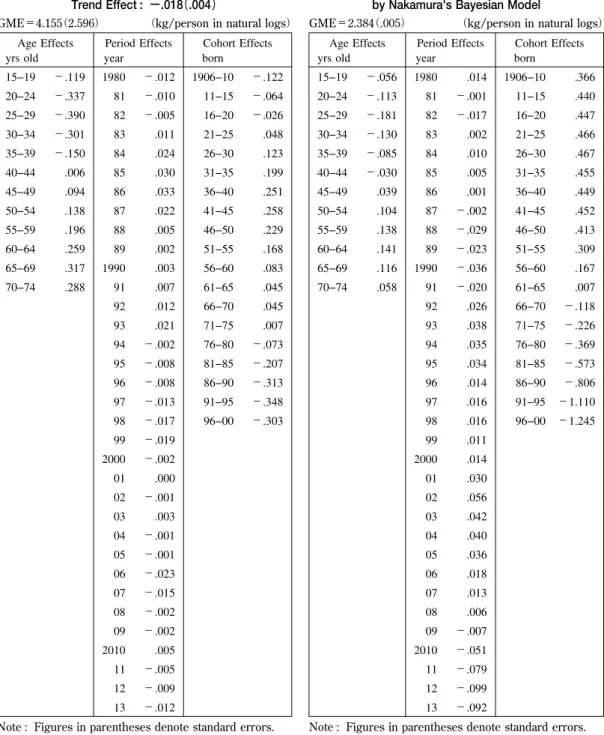
In implementing the “augmented cohort model” in the past few years to estimate demand elastici-ties of selected food products and applying the further refined models for this article, in particular, we have noticed that age and cohort effects derived from the traditional three factor, A/P/C model differ only marginally in some (the case of rice, Tables 6 A and B, for example) or moderately in other cases (the case of fish, Tables 7 A and B) from the parameter estimates derived from the models augmented with selected economic variables.
At this moment, we are in no position to assert which is superior in approximating age and co-hort effects or, from a different angle, whether demand elasticities determined simultaneously in the augmented model should be more plausible than the ones estimated in “two-steps”, using the pe-riod effects as dependent variables. Answering this would entail an experiment process using simu-lated data, in addition to further mathematical examinations, if any.
slope and annual fluctuations. Unless we possess any a-priori background information either for negative or positive trend effects, we may need to hesitate to apply T favorably in our augmented cohort model at this stage (so, Tables 6−9 C are not used for our projections).
4. Predicting Individual Consumption by Age, Synthesizing Age and
Cohort Effects
In the conventional A/P/C cohort modelling, per capita consumption of any selected product by individual of i years old at time t (Xit) is approximated as follows.
Xit=B+Ai+Pt+Ck+eit (1) where
B=grand mean effect
Ai=age effect attributable to age i yeas old Pt=period effect attributable to time t
Ck=cohort effect attributable to (birth) cohort k eit=error term
When we specify age, i, and time, t, birth cohort, Ckis automatically determined, since k = t − i. A group of individuals of 25 to 29 of age at the year 1980, for example belong to the cohort born in the years of 1951 to 1955, who moved the next age cell of 30−34 years old in 1985, −−−, the age cell of 55−59 years old in 2010, and will age to 60−64 and 65−69 years old in 2015 and 2020, respectively. In the case of fresh fish, for example, per capita consumption of this cohort in the year 2020, can be predicted as :
2.384+0.116+P2020+0.309=2.809+P2020in natural logs, or 16.59+exp (P2020) kg, according to the pa-rameter estimates provided in Table 7 A. The period effect attributable to the year 2020 is unknown at this moment but should not be far from the 4 year average of 2010−2013, −.080 in natural log, so that 2010 consumption would be 2.729 in log term, or 15.32kg per person per year.
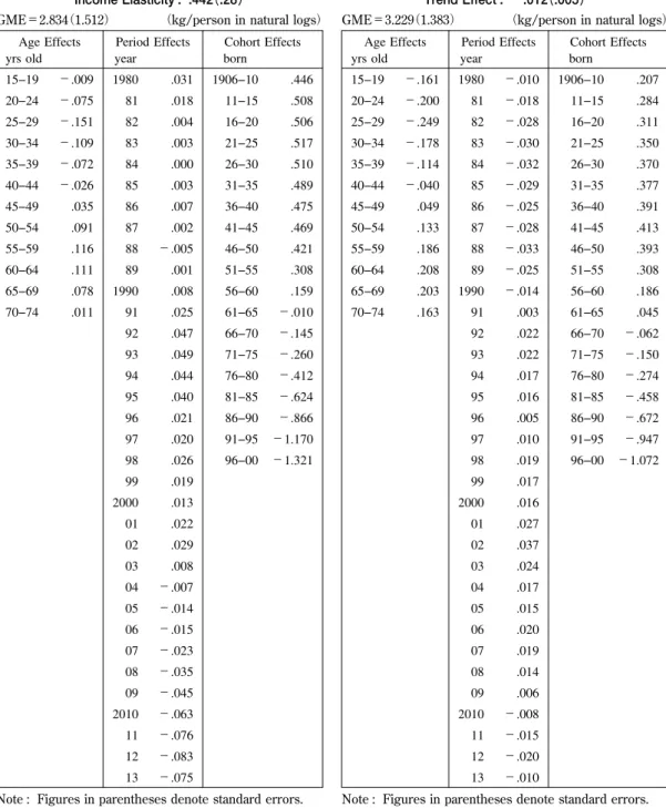
Per capita quantities of individual at-home consumption of rice, fish, meat and vegetables, respec-tively, by age classified in 5 year bracket from 15−19, 20−24, ―, 65−69, and 70−74 years old are pre-dicted for the years of 2015 and 2020, after the fashion prescribed in the preceding paragraph and provided in Table 10. Economic variables are not incorporated in the age and cohort estimation in Table 10. Both age and cohort effects are assumed to be unchanged over the entire period in ques-tion from 1980 to 2020 but period effects are variable over time and we are not sure whether they will be close to what they were in the latest years of 2010−2013, if the economic conditions are as-sumed unchanged. Observing the period effects provided in the middle column of Tables 6 A to 9 A, it looks plausible that both 2015 and 2020 would be close to the latest 4−5 years in respect to period effects for fish and vegetables and that the period effects would be declining slightly in the case of rice, whereas the opposite would be the case with meat. The period effects assigned to 2015 and 2020 in our calculations for Table 10 are : −0.153 and −0.172 for rice, 0.08 and 0.08 for fish, 0.17 and 0.27 for meat and 0.0 and 0.0 for vegetables, respectively.
Table 6A Rice Consumption Decomposed into Age, Period, and Cohort Effects, 1980-2013
by Nakamura's Bayesian Model
GME=3.465(.005) (kg/person in natural logs) Age Effects yrs old Period Effects year Cohort Effects born 15−19 .089 20−24 −.165 25−29 −.256 30−34 −.206 35−39 −.093 40−44 .025 45−49 .074 50−54 .081 55−59 .101 60−64 .126 65−69 .145 70−74 .079 1980 .255 81 .244 82 .232 83 .228 84 .214 85 .201 86 .188 87 .140 88 .079 89 .058 1990 .041 91 .032 92 .020 93 .016 94 −.052 95 −.064 96 −.062 97 −.068 98 −.068 99 −.081 2000 −.057 01 −.062 02 −.076 03 −.086 04 −.114 05 −.123 06 −.135 07 −.124 08 −.099 09 −.113 2010 −.111 11 −.129 12 −.152 13 −.170 1906−10 .200 11−15 .244 16−20 .241 21−25 .277 26−30 .315 31−35 .352 36−40 .366 41−45 .336 46−50 .268 51−55 .169 56−60 .045 61−65 −.031 66−70 −.069 71−75 −.145 76−80 −.263 81−85 −.435 86−90 −.580 91−95 −.655 96−00 −.636
Note : Figures in parentheses denote standard errors.
Table 6B Rice Consumption Decomposed into Age,
Period, and Cohort Effects, with no Trend, 1980-2013 by Saegusa's Augmented Bayesian Model
Elasticity of Rice P : −.056(.115); Elasticity of Fish P. : .722(.413) Elasticity of Meat P. : .114(.339)
Income Elasticity : −.879(.363)
GME=4.305(3.116) (kg/person in natural logs) Age Effects yrs old Period Effects year Cohort Effects born 15−19 .101 20−24 −.155 25−29 −.248 30−34 −.201 35−39 −.090 40−44 .026 45−49 .073 50−54 .077 55−59 .095 60−64 .118 65−69 .135 70−74 .067 1980 .106 81 .101 82 .098 83 .111 84 .120 85 .119 86 .117 87 .100 88 .077 89 .072 1990 .069 91 .069 92 .068 93 .074 94 .030 95 .019 96 .014 97 −.001 98 −.017 99 −.035 2000 −.022 01 −.034 02 −.046 03 −.050 04 −.065 05 −.081 06 −.110 07 −.109 08 −.103 09 −.116 2010 −.114 11 −.140 12 −.156 13 −.166 1906−10 .217 11−15 .260 16−20 .256 21−25 .290 26−30 .326 31−35 .361 36−40 .373 41−45 .340 46−50 .270 51−55 .169 56−60 .044 61−65 −.035 66−70 −.075 71−75 −.153 76−80 −.273 81−85 −.448 86−90 −.595 91−95 −.672 96−00 −.656
Table 7A Fish Consumption Decomposed into Age, Period, and Cohort Effects, 1980-2013
by Nakamura's Bayesian Model
GME=2.384(.005) (kg/person in natural logs) Age Effects yrs old Period Effects year Cohort Effects born 15−19 −.056 20−24 −.113 25−29 −.181 30−34 −.130 35−39 −.085 40−44 −.030 45−49 .039 50−54 .104 55−59 .138 60−64 .141 65−69 .116 70−74 .058 1980 .014 81 −.001 82 −.017 83 .002 84 .010 85 .005 86 .001 87 −.002 88 −.029 89 −.023 1990 −.036 91 −.020 92 .026 93 .038 94 .035 95 .034 96 .014 97 .016 98 .016 99 .011 2000 .014 01 .030 02 .056 03 .042 04 .040 05 .036 06 .018 07 .013 08 .006 09 −.007 2010 −.051 11 −.079 12 −.099 13 −.092 1906−10 .366 11−15 .440 16−20 .447 21−25 .466 26−30 .467 31−35 .455 36−40 .449 41−45 .452 46−50 .413 51−55 .309 56−60 .167 61−65 .007 66−70 −.118 71−75 −.226 76−80 −.369 81−85 −.573 86−90 −.806 91−95 −1.110 96−00 −1.245
Note : Figures in parentheses denote standard errors. Table 6C Rice Consumption Decomposed into Age,
Period, and Cohort Effects, with Linear Trend, 1980-2013 by Saegusa's Augmented Bayesian Model Elasticity of Rice P : −.121(.100); Elasticity of Fish
P. : .605(.350)Elasticity of Meat P. : .120(.270) Income Elasticity : −.591(.305)
Trend Effect : −.018(.004)
GME=4.155(2.596) (kg/person in natural logs) Age Effects yrs old Period Effects year Cohort Effects born 15−19 −.119 20−24 −.337 25−29 −.390 30−34 −.301 35−39 −.150 40−44 .006 45−49 .094 50−54 .138 55−59 .196 60−64 .259 65−69 .317 70−74 .288 1980 −.012 81 −.010 82 −.005 83 .011 84 .024 85 .030 86 .033 87 .022 88 .005 89 .002 1990 .003 91 .007 92 .012 93 .021 94 −.002 95 −.008 96 −.008 97 −.013 98 −.017 99 −.019 2000 −.002 01 .000 02 −.001 03 .003 04 −.001 05 −.001 06 −.023 07 −.015 08 −.002 09 −.002 2010 .005 11 −.005 12 −.009 13 −.012 1906−10 −.122 11−15 −.064 16−20 −.026 21−25 .048 26−30 .123 31−35 .199 36−40 .251 41−45 .258 46−50 .229 51−55 .168 56−60 .083 61−65 .045 66−70 .045 71−75 .007 76−80 −.073 81−85 −.207 86−90 −.313 91−95 −.348 96−00 −.303
Table 7C Fish Consumption Decomposed into Age, Period, and Cohort Effects, with Linear Trend, 1980-2013
by Saegusa's Augmented Bayesian Model Elasticity of Fish P : −.723(.157); Elasticity of Meat
P. : .077(.163)Elasticity of Vege P. : −.127(.080) Income Elasticity : .613(.262)
Trend Effect : −.012(.005)
GME=3.229(1.383) (kg/person in natural logs) Age Effects yrs old Period Effects year Cohort Effects born 15−19 −.161 20−24 −.200 25−29 −.249 30−34 −.178 35−39 −.114 40−44 −.040 45−49 .049 50−54 .133 55−59 .186 60−64 .208 65−69 .203 70−74 .163 1980 −.010 81 −.018 82 −.028 83 −.030 84 −.032 85 −.029 86 −.025 87 −.028 88 −.033 89 −.025 1990 −.014 91 .003 92 .022 93 .022 94 .017 95 .016 96 .005 97 .010 98 .019 99 .017 2000 .016 01 .027 02 .037 03 .024 04 .017 05 .015 06 .020 07 .019 08 .014 09 .006 2010 −.008 11 −.015 12 −.020 13 −.010 1906−10 .207 11−15 .284 16−20 .311 21−25 .350 26−30 .370 31−35 .377 36−40 .391 41−45 .413 46−50 .393 51−55 .308 56−60 .186 61−65 .045 66−70 −.062 71−75 −.150 76−80 −.274 81−85 −.458 86−90 −.672 91−95 −.947 96−00 −1.072
Note : Figures in parentheses denote standard errors. Table 7B Fish Consumption Decomposed into Age,
Period, and Cohort Effects, with no Trend, 1980-2013 by Saegusa's Augmented Bayesian Model
Elasticity of Fish P : −.673(.169); Elasticity of Meat P. : .232(.16) Elasticity of Vege P. : −.133(.085)
Income Elasticity : .442(.28)
GME=2.834(1.512) (kg/person in natural logs) Age Effects yrs old Period Effects year Cohort Effects born 15−19 −.009 20−24 −.075 25−29 −.151 30−34 −.109 35−39 −.072 40−44 −.026 45−49 .035 50−54 .091 55−59 .116 60−64 .111 65−69 .078 70−74 .011 1980 .031 81 .018 82 .004 83 .003 84 .000 85 .003 86 .007 87 .002 88 −.005 89 .001 1990 .008 91 .025 92 .047 93 .049 94 .044 95 .040 96 .021 97 .020 98 .026 99 .019 2000 .013 01 .022 02 .029 03 .008 04 −.007 05 −.014 06 −.015 07 −.023 08 −.035 09 −.045 2010 −.063 11 −.076 12 −.083 13 −.075 1906−10 .446 11−15 .508 16−20 .506 21−25 .517 26−30 .510 31−35 .489 36−40 .475 41−45 .469 46−50 .421 51−55 .308 56−60 .159 61−65 −.010 66−70 −.145 71−75 −.260 76−80 −.412 81−85 −.624 86−90 −.866 91−95 −1.170 96−00 −1.321
Table 8A Meat Consumption Decomposed into Age, Period, and Cohort Effects, 1980-2013
by Nakamura's Bayesian Model
GME=2.559(.003) (kg/person in natural logs) Age Effects yrs old Period Effects year Cohort Effects born 15−19 .183 20−24 −.023 25−29 −.073 30−34 −.076 35−39 −.041 40−44 .030 45−49 .071 50−54 .067 55−59 .045 60−64 .029 65−69 −.050 70−74 −.162 1980 .001 81 −.016 82 −.004 83 −.035 84 −.027 85 −.014 86 −.007 87 −.006 88 −.029 89 −.026 1990 −.030 91 −.028 92 −.026 93 −.007 94 −.007 95 −.004 96 −.018 97 −.015 98 −.023 99 −.009 2000 −.010 01 −.045 02 −.029 03 −.040 04 −.045 05 −.016 06 −.013 07 .009 08 .034 09 .074 2010 .078 11 .095 12 .101 13 .138 1906−10 −.185 11−15 −.195 16−20 −.186 21−25 −.149 26−30 −.085 31−35 −.026 36−40 .019 41−45 .075 46−50 .102 51−55 .084 56−60 .052 61−65 .050 66−70 .087 71−75 .123 76−80 .116 81−85 .078 86−90 .029 91−95 .005 96−00 .004
Note : Figures in parentheses denote standard errors.
Table 8B Meat Consumption Decomposed into Age, Period, and Cohort Effects, with no Trend, 1980-2013
by Saegusa's Augmented Bayesian Model Elasticity of Meat P : −.208(.149);
Elasticity of Fish P. : .164(.156) Elasticity of Vege P. : −.149(.070)
Income Elasticity : .020(.267)
GME=3.359(1.488) (kg/person in natural logs) Age Effects yrs old Period Effects year Cohort Effects born 15−19 .193 20−24 −.015 25−29 −.067 30−34 −.072 35−39 −.038 40−44 .031 45−49 .070 50−54 .064 55−59 .040 60−64 .022 65−69 −.059 70−74 −.172 1980 .031 81 .013 82 .009 83 −.010 84 −.002 85 −.002 86 −.004 87 −.010 88 −.022 89 −.019 1990 −.015 91 −.008 92 −.020 93 −.003 94 −.010 95 −.013 96 −.030 97 −.023 98 −.023 99 −.022 2000 −.034 01 −.067 02 −.048 03 −.045 04 −.041 05 −.018 06 −.017 07 .002 08 .030 09 .064 2010 .071 11 .085 12 .083 13 .120 1906−10 −.169 11−15 −.180 16−20 −.173 21−25 −.138 26−30 −.076 31−35 −.019 36−40 .025 41−45 .079 46−50 .104 51−55 .084 56−60 .050 61−65 .047 66−70 .082 71−75 .115 76−80 .107 81−85 .067 86−90 .016 91−95 −.009 96−00 −.012
Table 8C Meat Consumption Decomposed into Age, Period, and Cohort Effects, with Linear Trend, 1980-2013
by Saegusa's Augmented Bayesian Model Elasticity of Meat P : −.125(.165); Elasticity of Fish
P. : .184(.155)Elasticity of Vege P. : −.149(.070) Income Elasticity : −.073(.277);
Trend Effect : .005(.004)
GME=3.202(1.483) (kg/person in natural logs) Age Effects yrs old Period Effects year Cohort Effects born 15−19 .216 20−24 .004 25−29 −.052 30−34 −.061 35−39 −.032 40−44 .033 45−49 .068 50−54 .058 55−59 .030 60−64 .008 65−69 −.078 70−74 −.195 1980 .068 81 .046 82 .040 83 .020 84 .027 85 .026 86 .023 87 .015 88 .003 89 .003 1990 .003 91 .009 92 −.004 93 .015 94 .007 95 .002 96 −.019 97 −.018 98 −.022 99 −.024 2000 −.038 01 −.074 02 −.058 03 −.060 04 −.061 05 −.042 06 −.046 07 −.031 08 −.009 09 .025 2010 .030 11 .038 12 .035 13 .068 1906−10 −.133 11−15 −.146 16−20 −.143 21−25 −.113 26−30 −.054 31−35 −.002 36−40 .038 41−45 .087 46−50 .108 51−55 .084 56−60 .046 61−65 .038 66−70 .069 71−75 .098 76−80 .086 81−85 .041 86−90 −.013 91−95 −.043 96−00 −.049
Note : Figures in parentheses denote standard errors.
Table 9A Veges Consumption Decomposed into Age, Period, and Cohort Effects, 1980-2013
by Nakamura's Bayesian Model
GME=4.118(.003) (kg/person in natural logs) Age Effects yrs old Period Effects year Cohort Effects born 15−19 −.195 20−24 −.157 25−29 −.132 30−34 −.112 35−39 −.084 40−44 −.029 45−49 .031 50−54 .082 55−59 .128 60−64 .162 65−69 .174 70−74 .132 1980 .046 81 .041 82 .059 83 .041 84 .044 85 .050 86 .054 87 .035 88 .012 89 .004 1990 −.020 91 −.032 92 .007 93 −.011 94 −.011 95 −.009 96 .007 97 −.004 98 −.023 99 −.017 2000 −.014 01 −.031 02 −.016 03 −.046 04 −.047 05 −.039 06 −.046 07 −.027 08 .004 09 .021 2010 −.015 11 −.010 12 −.015 13 .007 1906−10 .144 11−15 .190 16−20 .212 21−25 .224 26−30 .246 31−35 .249 36−40 .225 41−45 .201 46−50 .144 51−55 .062 56−60 −.022 61−65 −.068 66−70 −.099 71−75 −.140 76−80 −.199 81−85 −.276 86−90 −.334 91−95 −.368 96−00 −.388
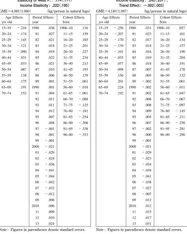
Table 9C Vege Consumption Decomposed into Age, Period, and Cohort Effects, with Linear Trend, 1980-2013
by Saegusa's Augmented Bayesian Model Elasticity of Vege P : −.382(.059); Elasticity of Fish
P. : −.043(.120)Elasticity of Meat P. : .159(.126) Income Elasticity : .242(.207);
Trend Effect : −.002(.003)
GME=4.140(1.087) (kg/person in natural logs) Age Effects yrs old Period Effects year Cohort Effects born 15−19 −.256 20−24 −.207 25−29 −.170 30−34 −.139 35−39 −.101 40−44 −.035 45−49 .037 50−54 .098 55−59 .156 60−64 .201 65−69 .224 70−74 .192 1980 .031 81 .023 82 .017 83 .014 84 .016 85 .019 86 .018 87 .007 88 .003 89 −.002 1990 −.002 91 .002 92 .008 93 .008 94 .009 95 .005 96 .007 97 −.002 98 .000 99 −.001 2000 −.021 01 −.029 02 −.023 03 −.034 04 −.038 05 −.041 06 −.038 07 −.027 08 −.007 09 .012 2010 .012 11 .015 12 .017 13 .031 1906−10 .057 11−15 .101 16−20 .134 21−25 .157 26−30 .190 31−35 .204 36−40 .191 41−45 .178 46−50 .132 51−55 .061 56−60 −.011 61−65 −.047 66−70 −.067 71−75 −.097 76−80 −.145 81−85 −.211 86−90 −.258 91−95 −.281 96−00 −.290
Note : Figures in parentheses denote standard errors. Table 9B Veges Consumption Decomposed into Age,
Period, and Cohort Effects, with no Trend, 1980-2013 by Saegusa's Augmented Bayesian Model
Elasticity of Veges P : −.382(.058); Elasticity of Fish P. : −.036(.118) Elasticity of Meat P. : .174(.111)
Income Elasticity : .222(.195)
GME=4.085(1.060) (kg/person in natural logs) Age Effects yrs old Period Effects year Cohort Effects born 15−19 −.216 20−24 −.174 25−29 −.145 30−34 −.121 35−39 −.090 40−44 −.031 45−49 .033 50−54 .087 55−59 .138 60−64 .175 65−69 .191 70−74 .152 1980 .036 81 .027 82 .021 83 .018 84 .019 85 .022 86 .021 87 .010 88 .006 89 .001 1990 .001 91 .004 92 .011 93 .011 94 .012 95 .007 96 .008 97 −.001 98 .001 99 −.001 2000 −.021 01 −.029 02 −.024 03 −.036 04 −.041 05 −.044 06 −.042 07 −.032 08 −.012 09 .006 2010 .006 11 .009 12 .010 13 .024 1906−10 .116 11−15 .159 16−20 .185 21−25 .201 26−30 .227 31−35 .234 36−40 .213 41−45 .193 46−50 .139 51−55 .061 56−60 −.018 61−65 −.061 66−70 −.088 71−75 −.125 76−80 −.181 81−85 −.254 86−90 −.308 91−95 −.338 96−00 −.353
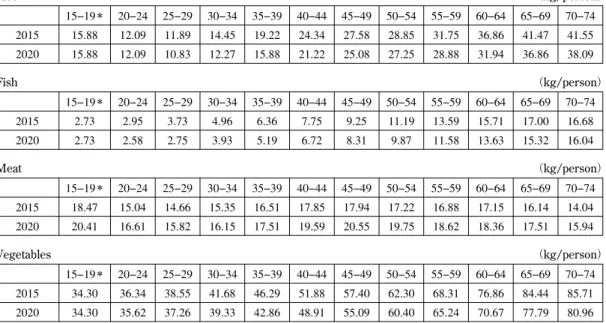
Table 10 Predicting per capita At-home Consumpton of Rice, Fish, Meat and Vegetables by Age Groups to 2015 and 2020 : Conventional A/P/C Model
Rice (kg/person) 15−19* 20−24 25−29 30−34 35−39 40−44 45−49 50−54 55−59 60−64 65−69 70−74 2015 15.88 12.09 11.89 14.45 19.22 24.34 27.58 28.85 31.75 36.86 41.47 41.55 2020 15.88 12.09 10.83 12.27 15.88 21.22 25.08 27.25 28.88 31.94 36.86 38.09 Fish (kg/person) 15−19* 20−24 25−29 30−34 35−39 40−44 45−49 50−54 55−59 60−64 65−69 70−74 2015 2.73 2.95 3.73 4.96 6.36 7.75 9.25 11.19 13.59 15.71 17.00 16.68 2020 2.73 2.58 2.75 3.93 5.19 6.72 8.31 9.87 11.58 13.63 15.32 16.04 Meat (kg/person) 15−19* 20−24 25−29 30−34 35−39 40−44 45−49 50−54 55−59 60−64 65−69 70−74 2015 18.47 15.04 14.66 15.35 16.51 17.85 17.94 17.22 16.88 17.15 16.14 14.04 2020 20.41 16.61 15.82 16.15 17.51 19.59 20.55 19.75 18.62 18.36 17.51 15.94 Vegetables (kg/person) 15−19* 20−24 25−29 30−34 35−39 40−44 45−49 50−54 55−59 60−64 65−69 70−74 2015 34.30 36.34 38.55 41.68 46.29 51.88 57.40 62.30 68.31 76.86 84.44 85.71 2020 34.30 35.62 37.26 39.33 42.86 48.91 55.09 60.40 65.24 70.67 77.79 80.96
*: Cohort effects for this age group at 2020 are assummed to be the same as those for 2015.
Table 11 Predicting per capita At-home Consumpton of Rice, Fish, Meat and Vegetables by Age Groups to 2015 and 2020 : Augmented Model
Rice (kg/person) 15−19* 20−24 25−29 30−34 35−39 40−44 45−49 50−54 55−59 60−64 65−69 70−74 2015 15.58 11.87 11.68 14.18 18.88 23.90 27.09 28.30 31.19 36.16 40.69 40.77 2020 15.58 12.06 10.82 12.24 15.85 21.20 25.05 27.19 28.82 31.91 36.78 38.02 Fish (kg/person) 15−19* 20−24 25−29 30−34 35−39 40−44 45−49 50−54 55−59 60−64 65−69 70−74 2015 2.73 2.97 3.73 4.96 6.36 7.75 9.24 11.19 13.59 15.69 17.00 16.68 2020 2.73 2.55 2.75 3.89 5.14 6.66 8.24 9.78 11.47 13.52 15.18 15.89 Meat (kg/person) 15−19* 20−24 25−29 30−34 35−39 40−44 45−49 50−54 55−59 60−64 65−69 70−74 2015 18.43 15.01 14.61 15.30 16.48 17.80 17.90 17.18 16.83 17.00 16.09 14.01 2020 20.13 16.35 15.56 15.88 17.29 19.28 20.21 19.43 18.32 18.05 17.22 15.69 Vegetables (kg/person) 15−19* 20−24 25−29 30−34 35−39 40−44 45−49 50−54 55−59 60−64 65−69 70−74 2015 34.09 36.09 38.28 41.39 45.92 51.52 57.00 61.81 67.90 76.25 83.76 85.03 2020 34.09 35.55 37.15 39.21 42.69 48.72 54.93 60.16 65.04 70.46 77.48 80.56
2015 and 2020, using the estimates of age and cohort effects by the augmented cohort model with the economic variables incorporated, on the assumption that the economic conditions, prices and household income would remain the same as in 2010−2013. Observing the movements of period ef-fects in the middle column of Tables 6 B to 9 B, the period efef-fects for fish and vegetables would stay the same as in 2010−2013, whereas those for rice would decline slightly from −0.18 to −0.229 and those for meat would increase from 0.152 to 0.24. Despite conspicuous differences in the parameter estimates of age and cohort effects between the conventional A/P/C and the augmented models, predicted consumption by age groups either by the conventional or augmented model has proved almost identical, regardless of the type of foods examined, as shown in Tables 10 and 11.
5. Concluding Results
The basic data used for the analyses depend on the FIES annual reports, which provide hold purchases of goods and services by households of two persons or more (single person house-holds are not covered) across the country from 1980 to 2013. In the case of rice, for example, rice consumed outside the home, or eating out, cooked rice in the form of obento or donburi, and Table 12 Estimates of Individual Consumption by Age Groups : Rice, Fish, Meat and Vegetables, The Base Year 2010
prepared-frozen rice to be cooked by microwave at-home, etc., purchased by households are not in-cluded. Some 30 years ago, it is estimated that uncooked rice purchased by households accounted for approximately 60% of total domestic rice supply, which gradually declined to less than 50% in the early 2010s, which may decline a little further to the 2020s. The percentage of (fresh) fish pur-chases for at-home use declined from 43% to 38% and that of (fresh) meat from 54% to 48%, whereas (fresh) vegetables have stayed nearly constant around 55% over the entire period (refer to Table 13 for the data sources). Our present analysis, however, has nothing to do with these tendencies.
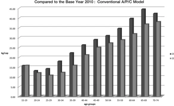
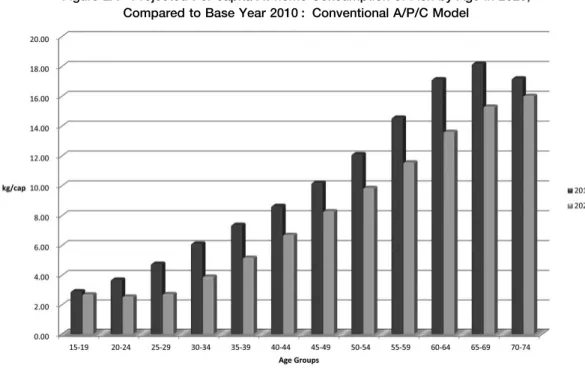
As graphically demonstrated by Figures 1 A&B to 4 A&B (see Tables 10 and 11 and Table 12 for numerical details), individual at-home (omitted hereafter) consumption of rice is projected to decline substantially, say 20 to 30% across the board, regardless of the age groups from 2010 to 2020 ; quite similarly, that of fish will decline substantially across the board ; that of meat, however, is projected to increase considerably, around 20% or so, without regard to the age groups ; finally, that of vege-tables is projected to decline moderately, say around 10% across the board. Older people consume more rice and vegetables and substantially more fish than younger people and older generations are estimated to exhibit greater cohort effects than the newer generations. In view of these analytical findings, a rapid aging of the population as expected in Japan in the future tends to mitigate pro-jected decreases across the board in individual consumption of rice, fish and vegetables, thus bol-stering aggregate consumption for some time to come.
References
Blaylock, J.R. and D.M. Smallwood(1986)U.S. Demand for Food : Household Expenditures, Demographics, and Projec-tions, USDA/ERS, TB-1713, February.
Blisard, N., J.N. Variyam, and J. Cromartie(2003)Food Expenditures by U.S. Households : Looking Ahead to 2020, USDA/ERS, Agricultural Economic Report No.821.
Buse, R.C. and L.E. Salathe(1978)“Adult Equivalent Scales : An Alternative Approach,” American Journal of Agricul-tural Economics, 60, 460−468.
Chalfant, J.A. and J.M. Alston(1988)“Accounting for Changes in Tastes,” Journal of Political Economy, 96(2), 391− 410.
Fu, Wenjiang J.(2008)“A Smoothing Cohort Model in Age-Period-Cohort Analysis with Applications to Homicide
Ar-Table 13 Ratios of per Person Purchases as Reported
in FIES to per capita
Domestic Supply Provided in FBS : Rice, Fish, Meat and Vegetables, 1980, 1990, 2000, and 2010
(%)
Rice Fish Meat Vegetables
1980 58.4 42.3 53.5 55.9
1990 51.9 36.1 48.0 53.6
2000 48.3 35.3 44.0 55.8
2010 47.4 37.6 47.9 63.1
Figure 1A Projected Per capita At-home Cosumption of Rice by Age in 2020, Compared to the Base Year 2010 : Conventional A/P/C Model
Figure 2A Projected Per capita At-home Consumption of Fish by Age in 2020, Compared to Base Year 2010 : Conventional A/P/C Model
Figure 3A Projected Per capita At-home Consumption of Meat by Age in 2020, Compared to Base Year 2010 : Conventional A/P/C Model
Figure 3B Projected Per capita At-home Consumption of Meat by Age in 2020,
Figure 4A Projected Per capita At-Home Consumption of Vegetables by Age in 2020, Compared to Base Year 2010 : Conventional A/P/C Model
rest Rates and Lung Cancer Mortality Rates,” Sociological Methods & Research, 36, 327−361. Glenn, Norval D.(1977)Cohort Analysis, Sage Publications, Beverly Hills, CA.
Holford, Theodore R.(1983)“The Estimation of Age, Period, and Cohort Effects for Vital Rates,” Biometrics 39, 311− 324.
――(1991)“Understanding the Effects of Age, Period, and Cohort on Incidence and Mortality Rates,” Annual Reviews in Public Health, 12, 425−457.
Huang, J. and H. Bouis(2001)“Structural change in the demand for food in Asia : empirical evidence from Taiwan,” Agricultural Economics, 26, ELSVER, 57−69.
Japanese Government, Bureau of Statistics, Family Income and Expenditure Survey, Annual Report, various issues, To-kyo.
――, Ministry of Agriculture, Forestry and Fisheries. Food Balance Sheet, various issues, Tokyo.
――, Policy Research Institute, MAFF(2010), Projecting Future Food Expenditures in A Rapidly Aging Country of Ja-pan, Press Released in September <http : //www.maff.go.jp/j/press/kanbo/kihyo01/100927.html>
Kawaguchi, Tsunemasa(1996)Professor of Econometrics, Kyushu University, Fukuoka, Japan.
Lin, B-W, J.N.Variyam, J. Allshouse, and J. Cromartie(2003)Food and Agricultural Commodity Consumption in the United States : Looking Ahead to 2020, USDA/ERS, Agricultural Economic Report No.820.
Mason, W. and S. Fienberg(1985)Cohort Analysis in Social Research : Beyond the Identification Problem, New York : Springer-Verlag.
Mori, Hiroshi(eds.)(2001)Cohort Analysis of Japanese Food Consumption―New and Old Generations, Tokyo, Senshu University Press.
Mori, H. and T. Inaba(1997)“Estimating Individual Fresh Fruit Consumption by Age from Household Data, 1979 to 1994,” Journal of Rural Economics, 69(3),175−85.
Mori, H. and D.L. Clason, and J. Lillywhite(2006)“Estimating Price and Income Elasticities for Foods in the Pres-ence of Age-Cohort Effects,” Agribusiness : an International Journal , 22(2),201−17.
Mori, H., Y. Saegusa, and T. Kawaguchi(2008)“Measures to Overcome the Identification Problem in Cohort Analy-sis : Tests Using Simulated Data,” The Annual Bulletin of Social Science, No.42, The Institute for Social Science, Senshu University, 69−99(in Japanese).
Mori, H.. Kawaguchi and Y. Saegusa(2009)“Methodological Examinations of the Bayesian and IE Cohort Models, Using Simulated Data of Standard Cohort Tables,” Senshu University Economic Bulletin, Vol. 44, No.1, 105−134 (in Japanese).
Mori, H. and Y. Saegusa(2010)“Cohort Effects in Food Consumption : What They Are and How They Are Formed,” Evolutionary and Institutional Economics Review, 7(1),43−63.
Mori, H. and H. Stewart(2011)“Cohort Analysis : Ability to Predict Future Consumption―The Cases of Fresh Fruit in Japan and Rice in Korea,” The Annual Bulletin of Social Science, No.45, The Institute for Social Science, Sen-shu University, 153−173.
Mori, H. and Y. Saegusa(2011)“Estimating Demand Elasticities of Fresh Fruit and Fresh Vegetables, Using Aug-mented Cohort Model with Economic Variables,” Senshu University Economic Bulletin, Vol. 46, No.2, 31−53(in Japanese).
Mori, H., Y. Saegusa and J. Dyck(2012)“Estimating Demand Elasticities in a Rapidly Aging Society―The Cases of Selected Fresh Fruits in Japan,” The Annual Bulletin of Social Science, No.46, The Institute for Social Science, Senshu University, 123−144.
Mori, H. and Y. Saegusa(2013)“Estimating the Impacts of O-157 and BSE on At-home Consumption of Beef―Using Augmented Cohort Model,” The Annual Bulletin of Social Science, No.47, The Institute for Social Science, Senshu University, 157−182(in Japanese).
Mori, H., Y. Saegusa, and T. Inaba(2014)“Incorporating Cohort Analysis into a Demand System―At-home Consump-tion of Apples, Mandarins and a Few Other Fruits in the Winter Season,” Senshu University Economic Bulletin, Vol. 49, No.2, 31−53(in Japanese).
Nakamura, Takashi(1982)“A Bayesian Cohort Model for Standard Cohort Table Analysis,” Proceedings of Institute of Statistical Mathematics, 29(2),Tokyo, 77−97(in Japanese).
――(1986)“Bayesian Cohort Models for General Cohort Tables,” Annals of the Institute of Statistical Mathematics, 38, 353−370.
Price, David W.(1970)“Unit Equivalent Scales for Specific Food Commodities,” American Journal of Agricultural Eco-nomics, 52, 224−33.
――(1979)“Demographic Change and the Demand for Food : Discussion,” American Journal of Agricultural Econom-ics, 61, 1061−62.
Rodgers, W.L.(1982)“Estimable Functions of Age, Period, and Cohort Effects,” American Sociological Review 47, 774−87.
Saegusa, Y. and H. Mori(2012)“Estimating Demand Elasticities by Means of Augmented Cohort Model―The Cases of Beef and Wine,” Senshu University Economic Bulletin, Vol. 47, No.1, 1−22(in Japanese).
Salathe, Larry(1979)“The Effects of Changes in Population Characteristics on U.S. Consumption of Selected Foods,” American Journal of Agricultural Economics, 61, 1036−45.
Shahpar, C. and G. Li(1999)“Homicide Mortality in the United States, 1935−1994 : Age, Period, and Cohort Effects, American Journal of Epidemiology, 150(11),1213−1222.
Schrimper, R.A.(1979)“Demographic Changes and the Demand for Food : Discussion,” American Journal of Agricul-tural Economics, 61, 1058−60.
Southard, Leland(1987)“How Demographics Will Change Food Consumption by 2005,” USDA/ERS, Agricultural Outlook, April, pp. 34−37.
Stewart, Hayden and Noel Blisard(2008)“Are Younger Cohorts Demanding Less Fresh Vegetables?,” Review of Agri-cultural Economics, Vol. 30, No.1, 43−60.
Stewart, H., D. Dong, and A. Carlson(2013)Why Are Americans Consuming Less Fluid Milk? A Look at Generational Differences in Intake Frequency, USDA/ERS, Economic Research Report No.149, May.
Stigler George, and Gary Becker(1977)“De Gustibus Non Est Disputandum,” American Economic Review, Vol. 67, No.2, 76−90.
Tanaka, M., H. Mori and T. Inaba(2004)“Re-estimating per Capita Individual Consumption by Age from Household Data,” Japanese Journal of Rural Economics, Vol.6, 20−30.
Tanaka, M., Y. Saegusa, H. Mori, and T. Kawaguchi(2007). “Overcoming ‘Identification Problem’ in Cohort Analysis ―Comparison of Nakamura’s Bayesian and IE Models,” Economic Bulletin of Senshu University, Vol. 42, No.1, 1− 44(in Japanese).
Tango, T. and S. Kurashima(1987)“Age, Period and Cohort Analysis of Trends in Mortality from Major Diseases in Japan : Peculiarity of the Cohort Born in the Early Showa Era,” Statistics in Medicine, Vol. 6, 709−726.