九州大学学術情報リポジトリ
Kyushu University Institutional Repository
Topology of Random Geometric Complexes in Thermodynamic Regime
アクシェイ, ゴエル
https://doi.org/10.15017/2534381
出版情報:九州大学, 2019, 博士(数理学), 課程博士 バージョン:
権利関係:
Complexes in Thermodynamic Regime
Akshay Goel
Complexes in Thermodynamic Regime
A Dissertation Submitted to the Graduate School of Mathematics, Kyushu University as a Partial Fulfillment of the Requirements for the Degree of
Doctor of Philosophy in Applied Probability
By
Akshay Goel
Under the Supervision of
Professor Tomoyuki Shirai
June 2019
Acknowledgements
First and foremost, I would like to express my sincere gratitude to my supervisors Professor Tomoyuki Shirai and Dr. Khanh Duy Trinh for their valuable guidance, encouragement and for the umpteen number of discussions without which this thesis would not be possible. Although Dr. Trinh is not my official supervisor, he never made me feel so. I would also like to thank Professor Shirai for providing financial support to attend conferences, whenever needed. “The difference between science and religion is that in science, the experimenter and the object of an experiment are different and in religion, they are same.” I am very fortunate to touch both these dimensions in the three years of my Ph.D., and the full credit for this goes to both supervisors who gave me enough time and independence. I would also like to thank Dr. Kenkichi Tsunoda, who is not only the co-author in our work but also helped me a lot in clearing my doubts during the first and second years of my Ph.D. At that time, he was the Post Doctoral fellow under the supervision of Professor Shirai.
I want to thank my scholarship donor Japan International Cooperation Agency (JICA). They not only provided the full financial support including Tuition fees (un- der the name of JICA-Friendship scholarship) for these three years but also took care of us (JICA participants) by doing the monitoring meetings regularly. JICA has done for me more than my expectations. Thank you very much. I would also like to thank my JICA-Coordinator Ms. Akiko Sakono for being very calm and flexible with me in every situation. I would like to extend my sincere gratitude to the President of Kyushu University, the Dean of the Faculty of Mathematics and the Head of the De- partment of Mathematics for accepting me as a Ph.D. student in Kyushu University.
I want to thank the Indian Institute of Technology Hyderabad (IITH) and the Indian government to have collaborations with Japan and providing us (Indian students) the opportunity to study in Japan. At the same time, I would also like to thank my Master’s supervisor Dr. Balasubramaniam Jayaram, who encouraged me to pursue a Ph.D. from Japan.
My wholehearted gratitude goes to my family, especially to my elder brother Mr.
Abhishek Kumar Goel and my father Mr. Praveen Goel for accepting my decisions in life in the most understanding way and allowed me total freedom to do whatever I want to do. I would also like to thank my friend Ms. Sushma Kumari for being with me in all my ups and downs. I would also like to thank my dear friends Mohit, Abhishek, Vaibhav, Pradeep Mishra, Poornenth, Nagarjuna Asam, and many others.
Every talk with them makes the head fountain. Last but not least, I would like to
II
express my gratitude to the mother Earth, this holy life, each creature, and each being on this planet.
Abstract
The emerging research area known as random topology comprises theoretical results that characterize the asymptotic behavior of topological properties of random objects.
One aspect of this area is the study of random geometric complexes and their topo- logical properties called Betti numbers. Random geometric complexes, regarded as higher-dimensional generalizations of random geometric graphs, are generated from random points under specific deterministic rules. They are built on random points with non-random radius that depends on the number of points and usually goes to zero as the number of points goes to infinity. With the appropriate scaling of the radius, it is known that there are three main regimes: sparse regime, thermodynamic regime and dense regime, in which the limiting behavior of Betti numbers of random geometric complexes is totally different. In this thesis, we mainly concentrate on random ˇCech complexes and random Vietoris-Rips complexes, the typical types of random geometric complexes, and on the thermodynamic regime, the regime in which fundamental problems such as the law of large numbers and central limit theorem have not been completely understood yet.
We establish the strong law of large numbers for Betti numbers of random ˇCech complexes (and random Vietoris-Rips complexes) built onRN-valued binomial point processes and related Poisson point processes in the thermodynamic regime. Here, we consider both the case where the underlying distribution of the point processes is absolutely continuous with respect to the Lebesgue measure on RN (Euclidean setting) and the case where it is supported on a C1 compact manifold of dimension strictly less than N (manifold setting). The strong law is proved under the very mild assumption, which only requires that the common probability density function belongs to Lp spaces, for all 1 ≤ p < ∞. The limiting constant in our results is the integral of a function, which is the limit of the Betti numbers of random ˇCech complexes built on homogenous Poisson point processes onRN in the thermodynamic regime. Our result in the Euclidean setting is an improvement of an existing result in the sense that the stronger assumptions on the density function in the existing result are replaced by the mild assumption mentioned above. While our result in the manifold setting is new in the sense that the only existing result for Betti numbers in this setting is the linear growth of their expected value.
We also establish the strong law of large numbers for persistent Betti numbers of random ˇCech filtrations (and random Rips filtrations) built on scaled binomial point processes and related Poison point processes, in both the settings. These results
IV
are the generalizations of our results for usual Betti numbers. We also derive the vague convergence of persistence diagrams (in the same settings as for persistent Betti numbers) by considering them as counting measures. The approach used in our results is general enough to apply to other geometric complexes and their filtrations as well.
Introduction 1
1 Preliminaries 5
1.1 Topological preliminaries. . . 5
1.1.1 Simplicial homology . . . 6
1.1.2 Persistent homology . . . 10
1.1.3 Homotopy equivalence . . . 12
1.1.4 Geometric complexes. . . 13
1.1.5 Critical points . . . 15
1.2 Probabilistic preliminaries . . . 17
1.2.1 Specific examples of point processes . . . 21
1.2.2 Basic notions of convergence in probability . . . 25
1.3 Manifold theory. . . 26
2 Literature in brief 29 2.1 Introduction. . . 29
2.2 Betti numbers. . . 32
2.2.1 Sparse regime . . . 33
2.2.2 Thermodynamic regime . . . 35
2.2.3 Dense regime . . . 38
2.2.4 Riemannian manifolds . . . 40
2.2.5 Stationary point processes . . . 41
2.3 Critical points & Euler characteristic . . . 45
2.3.1 Sparse regime . . . 46
2.3.2 Thermodynamic regime . . . 47
2.3.3 Dense regime . . . 48
2.3.4 Stationary point processes . . . 50
2.4 Persistent Betti numbers & persistence diagrams . . . 51
3 Betti numbers in the thermodynamic regime 59 3.1 Introduction. . . 59
3.1.1 Main results. . . 59
3.1.2 Motivation for the assumptions on the metric . . . 63 V
VI CONTENTS
3.2 SLLN for simplex counts. . . 64
3.2.1 Euclidean setting . . . 64
3.2.2 Manifold setting . . . 73
3.3 SLLN for Betti numbers . . . 75
3.3.1 Euclidean setting . . . 75
3.3.2 Manifold setting . . . 84
3.4 Exponential decay of the limiting constant . . . 85
3.5 Conclusion & future directions . . . 87
4 Persistent Betti numbers and persistence diagrams 89 4.1 Introduction. . . 89
4.1.1 Main results. . . 89
4.2 SLLN for persistent Betti numbers . . . 92
4.3 Vague convergence of persistence diagrams. . . 94
4.3.1 General theory for vague convergence . . . 95
4.3.2 Euclidean setting . . . 100
4.4 Conclusion & future directions . . . 102
Bibliography 104
0.1 Illustration of gluing edges while constructing geometric complexes . . 1 0.2 Plot of Swiss roll data set . . . 2 0.3 Illustration of capturing the homology of a 2-dimensional annulus by
union of balls . . . 3 1.1 Pictorial representations of some simplicial complexes. . . 6 1.2 Example of a filtration and its 1st persistence diagram, and relationship
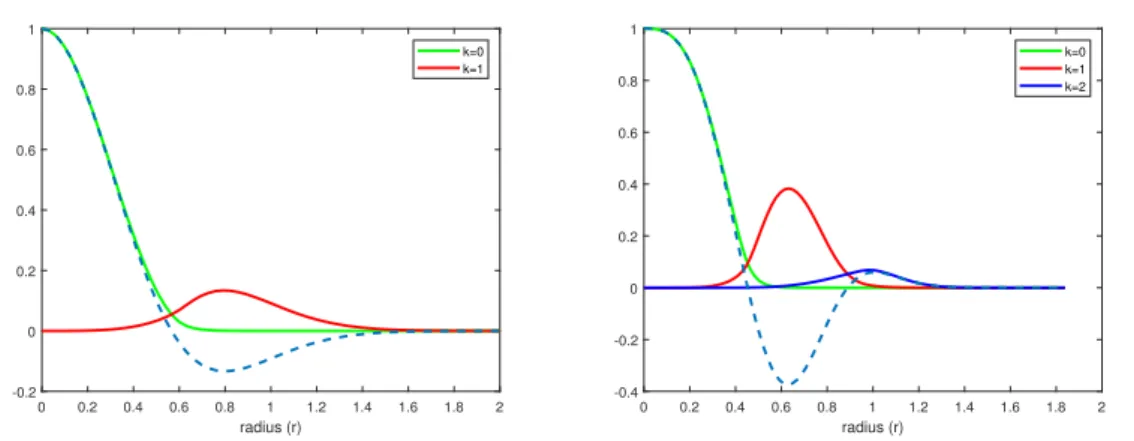
between persistent Betti numbers and persistence diagram . . . 11 1.3 A commutative diagram (for point processes) . . . 19 2.1 Illustration of different limiting regimes . . . 31 2.2 Illustration of the limiting constant ˆβk(N)(1, r) with N = 2 (left) and
N = 3 (right).. . . 36
VII
The following list describes several symbols and notations used in the thesis. Some notations, which are used locally in the thesis, are omitted from the list.
Algebraic Topology
K Simplicial complex
Sj(K) Number ofj-simplices in K βk(K) kth Betti number ofK
K A filtration of simplicial complexes βks,t(K) kth persistent Betti number ofK C(·)(C(·)) Cech complex ( ˇˇ Cech filtration)
VR(·) (VR(·)) Vietoris-Rips complex (Vietoris-Rips filtration)
K(·) κ-filtration
U(·) Union of balls
CPk(·) Number of critical points with indexk CPk(g)(·) Number of global critical points with indexk
CPk>(·) Number of critical points with index k whose critical values are greater than the parameter that will be specified in (·)
Probability
Λ Locally compact, second countable Hausdorff topological space B(Λ) Borelσ-field of Λ
R(Λ) Ring of relatively compact Borel sets of Λ M(Λ) Space of Radon measures on Λ
N(Λ) Space of integer-valued Radon measures on Λ IX
X NOTATIONS & SYMBOLS
Φ A general point process
λ(k)(·) kth factorial moment measure of a point process pk(·) kth joint intensity of a point process
λ(·) Intensity of a point process (= λ(1)(·)). Also used as a intensity function of a point process (= p1(·)). There is no ambiguity in this usage and it will be clear from the context.
Xn(Zn) Binomial point process in Euclidean setting (in manifold setting) Pn(Qn) Poissonized version of a binomial point process in Euclidean set-
ting (in manifold setting)
P(λ) Homogenous Poisson point process with intensity functionλ P(A) Probability of the event A
E[·] Expectation operator V[·] Variance operator
P oi(α) Poisson random variable with parameterα N(0,1) Standard normal distribution
Sets & Other symbols
N Natural numbers {0,1,2, . . .}
N¯ Extended natural numbers {0,1,2, . . .} ∪ {∞}
R Real numbers
R¯2 Extended plane
N orm Used to represent dimension of Euclidean spaces Leb(N)(A) N-dimensional Lebesgue measure of the set A⊂RN
|A| Cardinality of the set A A◦ Interior of the set A
∂A Boundary of the setA
Some notations
an=O(bn) if there exist a constantC >0 andn0>0 such thatan≤Cbn for all n≥n0
an= Θ(bn) if there exist constants c, C >0 and n0>0 such thatcbn≤an ≤ Cbn for all n≥n0
The emerging research area known as random topology comprises theoretical results that characterize the asymptotic behavior of topological properties of random objects [34, 35, 7, 10, 70, 30]. One aspect of this area is the study of random geometric complexes and their topological properties such as Betti numbers. This thesis is about the (asymptotic) behavior of topological properties of random geometric complexes in thethermodynamic regime. We can visualize a geometric complex in a 3-dimensional space as a shape built from such “elementary parts” as points, line segments, triangles, and tetrahedra by gluing them together along their faces. It means that we are only allowed to glue endpoints of line segments to endpoints of line segments, line segments to line segments and triangles to triangles (see for example Figure 0.1). There may be various ways to introduce the randomness in a geometric complex. In our work, however, a random geometric complex is always formed by first choosing a set of points randomly and then based on their position in the space, we draw line segments, triangles, tetrahedra, etc between them. In other words, random geometric complexes are generated from random points under certain deterministic rules. We are primarily interested in studying the homology (in particular, Betti numbers) and persistent homology (in particular, persistent Betti numbers) of these random complexes and their filtrations respectively. In addition to mathematical curiosity, such studies are also motivated by many issues in Manifold Learning (ML) and Topological Data Analysis (TDA).
a=d
b
c=f
e (a)
a
b
c d
e
f
(b)
Figure 0.1: The gluing of the edgesacand df of the triangles△abcand △def in (a) is correct, while in (b) is not correct.
1
2 INTRODUCTION
Figure 0.2: Plot of Swiss roll data set, which shows that each data point is inR3 but the data points live on a ‘sheet-like’ 2-dimensional manifold.
The field of ML is based on the idea that high dimensional data may live on or close to a submanifold of the ambient space whose dimension may be very less than that of the ambient space (see for instance Figure 0.2 as a toy example). If this assumption is true, then one would like to estimate the geometrical and topological properties (mainly homology) of this unknown manifold by the given data. One of the first results in this regard was given by Niyogi et al. [46]. They considered the set ofnpoints that are drawn uniformly and independently from a compact manifoldM embedded inRN (with given its conditional number). Then they showed that under certain conditions onnandr >0, the homology of the union of balls (inRN) of radius r around each point captures the homology ofM with high probability. Moreover, they were also able to capture the homology ofM in the case where Gaussian noise is added to every sampled point in their second paper [47]. Although the estimator in their results, i.e., the union of balls, is not a geometric complex, as we shall see, there is a complex (known as a ˇCech complex) which has the same homology as the union of balls. Similarly, there is another well-known geometric complex known as Vietoris-Rips complex that can also be used to estimate the topological properties of unknown manifold. Hausmann [28] and Latschev [42] have used this complex in this type of problem. Thus, by studying the homology of geometric complexes (either Cech or Vietoris-Rips) built on the random points of a manifold, one can developˇ a probabilistic null hypothesis for topological statistics. This direction of research was further extended in Balakrishnan et al. [2], Bobrowski and Mukherjee [10] and Bobrowski et al. [11].
From now onwards by a random geometric complex we mean either a random ˇCech complex or a random Vietoris-Rips complex. Generally, random geometric complexes are built on random points with some non-random radius. From the literature on random geometric complexes, we learn that while studying the asymptotic behavior of their topological properties such as homology, the non-random radius is a function of n (the number of points) whose limiting behavior after appropriate scaling, as n goes to infinity, can be categorized into three main limiting regimes: sparse regime, thermodynamic regime and dense regime. The asymptotic behavior of the topological
(a) (b) (c)
Figure 0.3: Illustration of capturing the homology of a 2-dimensional annulusMby union of balls denoted by ˆM: In (a), n= 100, r= 0.2 and β0(M)̸=β0( ˆM); in (b), n = 300, r = 0.2 and β1(M) ̸= β1( ˆM) (however, this is not visible in (b)); in (c), n= 1000, r = 0.2 and βk(M) =βk( ˆM) for all k≥0. This choice of parameterr is calculated using the main result of Niyogi et. al. [46].
properties of geometric complexes is totally different in each regime (for instance, see Figure 2.1). This point will be discussed in more detail in Section 2.1. Note that the tools used to determine the limiting behavior is each regime are also different.
Bobrowski and Mukherjee [10] has shown that the homology of the unknown manifold can be revealed by that of random ˇCech complexes in the dense regime. Moreover, there is an intuitive belief that dense regime is the only regime for homology inference.
However, it is not clear what happens in the thermodynamic regime since the basic questions such as law of large numbers and central limit theorem are not entirely understood yet. In the thesis, we answer the question of law of large numbers in the thermodynamic regime. Our main result is stated in Theorem 3.1. Since the limiting constant in Theorem3.1 is the integral of a function over the manifold and the integrand does not depend on the manifold, our result affirms the belief that dense regime is the only regime appropriate for homology inference.
Besides the above motivation from ML, our motivation also comes from the purely mathematical side, which is known as stochastic geometry. In stochastic geometry, the estimator in the results of Niyogi et al., i.e., the union of balls inRN of radius centered at random points, is a particular case of ‘Boolean model’. In general Boolean models, the radius is also random and independent of points. The geometric properties of the Boolean model such as volume and surface area have been well studied. Therefore, the next natural question arises about its topological features such as homology or Betti numbers. Furthermore, in stochastic geometry, weak and strong law of large numbers have been established for a general class of random variables that can be written as a sum of local functions [57,55]. Such random variables are said to be local statistics.
Here, the local functions encode the contribution from each point of the underlying point process. Simplex counts of random geometric complexes are examples of local statistics. However, Betti numbers do not belong to this class. Thus, the study of Betti numbers needs further development. We propose in this thesis an elementary
4 INTRODUCTION approach to show the strong law of large numbers of Betti numbers.
On the other hand, with the pioneering works of Edelsbrunner et al. [20], and Zomorodian and Carlsson [71], we now have an established research field known as TDA (see [14,15] on a excellent introduction of TDA). Recently, TDA has been also applied in various applications such as characterization of the hierarchical structure of amorphous solids and pore geometry of rocks, analyzation of protein binding, etc [29, 38,65, 32,48]. It is well understood from applications in TDA that considering only homology will not be enough. It is important to see how persistent the ‘holes’
are, which constitutes the theory of persistent homology. Furthermore, persistent homology is also useful in ML. In the results of Niyogi et al., we need some information about the geometry of the unknown manifold such as its conditional number to find out the correct choice of the parameter r so that the union of balls of radius r can capture the homology of the manifold. In many cases, however, we do not have this information to find the correct choice ofr. Via persistent homology, one can overcome this issue.
The main idea behind persistent homology is to consider the whole range ofr in- stead of some particular value. Whenr= 0, we havennumber of distinct points. As r increases, the homology starts changing non-monotonously (except 0th homology that is connected components, which only decreases asr increases) until the union of balls becomescontractible. In persistent homology, we keep track of these changes and finally, visualize these changes with the help of so-called persistence diagrams. The
‘holes’ whose persistence is ‘small’ consider as the noise, and the remaining ‘holes’
are considered as the true topological features of the unknown manifold. The most important feature of persistent homology is its stability under perturbations of the data, i.e., small changes in the data create at most small changes in the persistent ho- mology [19, Chapter VIII]. In the thesis, we do not focus on TDA or any applications at all. Instead, we derive some asymptotic results for persistent Betti numbers and persistence diagrams. These results are obtained using the tools developed for prov- ing the results for usual Betti numbers. These results for persistent Betti numbers and persistence diagrams may be of practical interest.
The thesis is organized into four chapters. Chapter1contains necessary topolog- ical and probabilistic preliminaries that are required in our work. Chapter2contains a brief survey of the existing literature of random topology. There we see what results we have in the literature and where the new results in this thesis fit into the litera- ture. Chapter 3 contains our main work in which we establish a strong law of large numbers for Betti numbers in the thermodynamic regime. In Chapter4, we consider particular type of filtrations of random geometric complexes and derive asymptotic results for persistent Betti numbers and persistence diagrams.
Preliminaries
Random topology is a combination of algebraic topology and probability. In this chapter, we collect basic concepts and corresponding results from these two fields that led to the foundation of our work. We start with the preliminaries of algebraic topology.
1.1 Topological preliminaries
In this section, we introduce only those concepts and results from algebraic topology that are relevant to our work. We begin with the definition of a simplicial complex.
Definition 1.1 (Simplicial complex). Let V = {v1, v2, . . . , vn} be a finite set of points (not necessary to be the points in a metric space). A simplicial complex with vertex setV is a collectionK of nonempty subsets ofV such that
(i) {vi} ∈ Kfor all i∈ {1,2, . . . , n}; (ii) ifσ∈ K and∅ ̸=τ ⊂σ thenτ ∈ K.
Note that the vertex set of a simplicial complex will always be finite in this thesis.
The elements in K are known as its simplices. The dimension dim(σ) of a simplex σ ∈ K is its cardinality minus 1, i.e., dim(σ) =|σ| −1. The dimension dim(K) of a simplicial complex K is maxσ∈Kdim(σ). If dim(σ) =j then we say that σ ∈ K is a j-simplex ofK. The set of allj-simplices inKand its cardinality are denoted byK(j) and Sj(K), respectively, i.e., Sj(K) :=|K(j)|. A subcollection ˜K ⊂ Kthat itself is a simplicial complex is said to be asubcomplex ofK.
Example 1.2. Let ˜K and K be two simplicial complexes, where K˜ ={
{v1},{v2},{v3},{v1, v2},{v2, v3},{v3, v1}} K={
{v1},{v2},{v3},{v1, v2},{v2, v3},{v3, v1},{v1, v2, v3}} .
In this example, dim( ˜K) = 1, dim(K) = 2, ˜K is a subcomplex of K, ˜K(0) =K(0) and K˜(1)=K(1).
5
6 1.1. TOPOLOGICAL PRELIMINARIES
v1 v2
v3
v1 v2
v3
(a)
v1 v2
v3
v4
(b)
Figure 1.1: Figure (a) represents pictorially ˜K (empty triangle) and K (full triangle) in Example 1.2 respectively. Figure (b) illustrates that the two 1-dimensional holes generated by taking the boundaries of the triangles
△v1v2v3 and △v1v2v4 are equivalent. The corresponding simplicial complex is {{v1},{v2},{v3},{v4},{v1, v2},{v2, v3},{v3, v1},{v1, v4},{v2, v4},{v4, v3},{v1, v4, v3} ,{v2, v4, v3}}
.
1.1.1 Simplicial homology
Homology is a mathematical setup that captures ‘holes’ or ‘non-trivial cycles’ in a topological space. A complete introduction of this topic can be found in [27,44]. The homology of a topological spaceXis a sequence of abelian groups{Hk(X)}∞k=0, where for eachk,Hk(X) is known as thekth homology group of X. The rank ofHk(X) is known as thekthBetti number, denoted byβk(X). We are primarily interested in the homology of a simplicial complex, which is also known as simplicial homology. In the case of a general topological space such as sphere or torus, one can first triangulate the space to obtain a simplicial complex and then apply the simplicial homology or can use the so-called singular homology alternatively. Here, instead of discussing the triangulation or the singular homology, we note Betti numbers of sphere and torus as examples and two general facts, which are enough for our purposes. A two- dimensional sphere S2 has β0(S2) = 1, β1(S2) = 0, β2(S2) = 1 and βk(S2) = 0 for all k ≥ 3. In general, an m-dimensional sphere Sm has β0(Sm) = βN(Sm) = 1 and βk(Sm) = 0 for all k∈N\ {0, m} [27, cf. Corollary 2.14]. A 2-dimensional torus T2 has β0(T2) = β2(T2) = 1, β1(T2) = 2 and βk(T2) = 0 for all k ≥3. In general, an m-dimensional torus hasβk(Tm) =(m
k
)for 0≤k≤mand zero for allk≥m+1. The facts are as follows: (i) ifX has dimensionm thenHk(X) is trivial for all k≥m+ 1 and so βk(X) = 0 for all k ≥m+ 1; (ii) ifX is a subset of RN and has dimension less than or equals to N then Hk(X) is trivial for all k ≥ N. In case of a sphere Sm (or a Torus Tm), these two facts are same since they can be embedded inRm+1. However, in case of a N-dimensional annulus that is a subset of RN, the fact (ii) is more stronger than (i), while there exist m-dimensional Riemannian manifolds that can be only embedded inRN forN > m+ 1, and so for these spaces, the fact (i) is more stronger than (ii). It is important to note that whenX is a simplicial complex with vertex set that is a subset ofRN, its dimension has no relation withRN because
its dimension is the maximum of the dimensions of its simplices, which can be made arbitrarily large.
We first intuitively discuss the simplicial homology. LetKbe a simplicial complex.
The zeroth homology H0(K) is generated by the elements representing connected components of K. While for k≥1,Hk(K) is generated by the elements representing k-dimensional holes that are not equivalent to each other. Informally, ak-dimensional hole should be thought as the result of taking the boundary of a k+ 1 dimensional empty body. For example, the boundary of an empty triangle should be regarded as a 1-dimensional hole whereas the boundary of a full triangle should not be (see Figure 1.1(a)). Two or more holes of the same dimension are equivalent if they can be con- tinuously deformed into each other. For instance, the two 1-dimensional holes formed by taking the boundaries of the triangles△v1v2v3 and △v1v2v4 in Figure 1.1(b) are equivalent and should be regarded as one hole. Hence, β0(K) counts the number of connected components ofKandβk(K), fork≥1, counts the number ofk-dimensional holes inK that are not equivalent to each other.
We now make the above ideas concrete. To do this, we need to assign orientations on simplices. Let K be a simplicial complex and σ = {v1, v2, . . . , vk+1} ∈ K be a k-simplex. By considering it as an ordered set, we have a total (k+ 1)! orderings on σ. For k ≥ 1, define two orderings on σ to be equivalent if they differ by an even permutation. In this way, we get two equivalent classes such that each ordering onσ belongs to one of them. Each equivalent class is called anoriented simplex. Note that in the case of a 0-simplex, we have only one equivalent class. Let us fix an ordering on the vertex set. We denote the equivalent class that contains the natural ordering (i.e., the ordering corresponding to the ordered vertex set) onσ by⟨v1, v2, . . . , vk+1⟩=:⟨σ⟩ and the other by adding a minus sign, i.e., by −⟨v1, v2, . . . , vk+1⟩. Let F be a field.
Consider the following set for eachk≥0, Ck(K) ={∑
ai⟨σi⟩:σi ∈ K(k), ai∈F} .
These spaces are called chain groups. In general, coefficients ai may not be the elements of a field. However, we always assume the coefficients belong to an arbitrary, fixed fieldF. In this case,Ck(K) becomes the vector space overF. For computational purposes, it is convenient to work with the fieldF2 ={0,1} because the orientation of simplices is not required in this case. Note that since K(k) is always an empty set fork <0 ork >dim(K),Ck(K) is a trivial space.
To relate these spaces, we define a linear map called theboundary map∂k:Ck(K)→ Ck−1(K), which is the linear extension of
∂k(⟨v1, v2, . . . , vk+1⟩) =
k+1∑
i=1
(−1)i⟨v1, . . . ,vˆi, . . . , vk+1⟩,
where ˆvi means the removal of vi. Thus, we obtain a sequence of chain groups and boundary maps, indexed byk. This sequence is called thechain complex of K.
· · ·−−−−→∂k+2 Ck+1(K)
∂k+1
−−−−→Ck(K)
∂k
−−−−→Ck−1(K)
∂k−1
−−−−→ · · ·
8 1.1. TOPOLOGICAL PRELIMINARIES LetZk(K) = ker∂k and Bk(K) = im∂k+1. The fundamental lemma of homology [44, Lemma 5.3] says that ∂k◦∂k+1 = 0, which implies Bk(K) ⊂ Zk(K), for all k ≥ 0.
The homology ofK is defined as follows:
Definition 1.3 (Homology & Betti number). The kth homology group Hk(K) of a simplicial complexK is the quotient space
Hk(K) =Zk(K)/Bk(K).
Thekth Betti numberβk(K) is the dimension of Hk(K), i.e., βk(K) = dim(Hk(K)) = dim(Zk(K))−dim(Bk(K)).
Example1.4. Let us see by an example how the intuitive explanation of the homology is achieved by the above definition. Letp = −⟨v2, v3⟩+⟨v1, v3⟩ − ⟨v1, v2⟩ ∈ C1(K).
Then p ∈ Z1(K) since ∂1(p) = 0 and it is also the boundary of a 2-dimensional oriented simplex⟨v1, v2, v3⟩ (a triangle) since ∂2(⟨v1, v2, v3⟩) =p. Now p generates a 1-dimensional hole only if{v0, v1, v2}∈ K/ or in other words, ifp /∈B1(K). So taking quotientZ1(K)/B1(K), is one way to count the number of 1-dimensional holes in K as Z1(K)\B1(K) can do the same. However, taking quotient Z1(K)/B1(K) is the only way to count the number of non-equivalent holes. This is clear by the following example.
LetK be the simplicial complex in Figure1.1(b). Letp1 andp2 be the boundaries of triangles△v1v2v3 and △v1v2v4 respectively, i.e., p1 =−⟨v2, v3⟩+⟨v1, v3⟩ − ⟨v1, v2⟩ and p2 = −⟨v2, v4⟩+⟨v1, v4⟩ − ⟨v1, v2⟩. Adding and subtracting ⟨v3, v4⟩ in p1 −p2
gives∂2(⟨v1, v4, v3⟩+⟨v2, v3, v4⟩). Since{v1, v4, v3},{v2, v3, v4} ∈ K,p1−p2∈B1(K).
Thus, by taking quotientZ1(K)/B1(K), 1-dimensional holes generated by p1 and p2
will be counted as one, which is required.
Note that the homology spaces are independent of the orientation of simplices.
We now state some important properties of Betti numbers that will be used in our work. Betti numbers are generally the global phenomena, which makes them hard to deal with directly in the random setting. Thus, we need some structures, which must be the local phenomena and can also be used to estimate Betti numbers. One example of such structures are simplex countsSj(·). Betti numbers can be estimated through them as follows.
Lemma 1.5. LetK,K˜ be any two finite simplicial complexes such that K ⊂ K˜ . Then for everyk≥0,
βk(K)−βk( ˜K)≤
k+1∑
j=k
(Sj(K)−Sj( ˜K)) .
Lemma 1.5 is proved for k ≥ 1 in [70, Lemma 2.2]. We here present a more fundamental proof (using linear algebra) of this lemma fork≥0 from [62].
Proof. It is clear that Ck(K) is a vector space with basis K(k). Since ∂k is a linear map from Ck(K) to Ck−1(K), we can represent ∂k of by a Sk−1(K)×Sk(K) matrix M atk(K), whose each element is in F. Then dim(Bk(K)) = rank(M atk+1(K)) and dim(Zk(K)) =Sk(K)−rank(M atk(K)) (by rank-nullity theorem). So,
βk(K) =Sk(K)−rank(M atk(K))−rank(M atk+1(K)). (1.1) Let ˜K be a subcomplex of K. By arranging the elements in bases of Ck(K) and Ck−1(K) such that the first elements coincide with the elements in bases of Ck( ˜K) and Ck−1( ˜K) respectively, M atk(K) has the following form
M atk( ˜K)
∗ 0
It follows from the above form ofM atk( ˜K) that
0≤rank(M atk(K))−rank(M atk( ˜K))≤Sk(K)−Sk( ˜K). (1.2) Combining Expressions (1.1) and (1.2) yields the desired result. This completes the proof.
From Equation (1.1), we have that
βk(K)≤Sk(K). (1.3)
We also have the finite additivity of Betti numbers, a desirable property required in probability. Let K1,K2. . . ,Kn be a finite number of disjoint simplicial complexes.
Then for allk≥0,
βk ( n
∪
i=1
Ki
)
=
∑n i=1
βk(Ki). (1.4)
Equation (1.4) can be proved similarly as Lemma 1.5 is proved. Betti numbers are topological invariants, i.e., invariant under homeomorphisms. Another important topological invariant is the Euler characteristic of a topological space. It has many equivalent definitions, one of them for simplicial complexes is the following.
Definition 1.6 (Euler characteristic). LetK be a finite simplicial complex. The Euler characteristic χ(K) is the alternating sum
∑(−1)jSj(K).
It can be easily shown that [27, cf. Theorem 2.44]
χ(K) =∑
(−1)kβk(K).
We conclude this subsection with the following remark.
Remark 1.7. In this thesis, we study the homology of simplicial complexes in random setting. Similarly, one can also study the homology of cubical sets, known as cubical homology in random setting. This study is recently carried out by Hiraoka and Tsunoda in [31]. Also, see [33] for a good introduction of cubical homology.
10 1.1. TOPOLOGICAL PRELIMINARIES 1.1.2 Persistent homology
We have already seen the motivation, or rather need, to study persistent homology in the introduction of the thesis. In this subsection, we make the mathematical ideas behind persistent homology concrete. A basic introduction of this topic can be found in [19]. Here, the theory is mostly taken from [30]. We study persistent homology for a filtration of simplicial complexes. The definition of filtration is as follows:
Definition 1.8(Filtration). Afiltration of simplicial complexes is a one parameter family of simplicial complexes, denoted by{Kr}r≥0, such that if 0≤r ≤ sthen Kr
is a subcomplex ofKs and for all r≥0,Kr=∩s>rKs.
We always assume that K0 in the filtration is the set of vertices, i.e., contains only 0-simplices. Given a filtrationK:={Kr}r≥0, the kth homology ofKr,Hk(Kr), changes asr increases. These changes are tracked by a linear map induced from the inclusionKs,−→ Kt, where 0≤s≤t, denoted by fks,t:Hk(Ks) −→Hk(Kt). Basically, if the kth homology cycle [c] of Ks still alive at Kt then fks,t([c]) ̸= 0, otherwise fks,t([c]) = 0. Note that it is not necessary that fks,t([c]) = [c] if it is non-zero (see Example1.11).
Definition 1.9 (Persistent homology & persistent Betti numbers). The kth persistent homology of K, denoted by Hk(K), is defined by the family of the images of linear mapsfks,t, 0≤s≤t, i.e, Hk(K) :={imfks,t:s≤t∈R}. Thekth persistent Betti numbers are the dimensions of the vector spaces imfks,t,βks,t(K) = dim(imfks,t).
Therefore, the intuitive meaning of βks,t(K) is the number ofk-dimensional holes that appear before or atsand still alive attin the filtrationK. Note thatHk(Ks) = imfks,s, so βks,s(K) =βk(Ks) and in general,
βks,t(K) = dim
( Zk(Ks) Zk(Ks)∩Bk(Kt)
) . This is because
imfks,t∼= Hk(Ks) kerfks,t =
Zk(Ks) Bk(Ks) Zk(Ks)∩Bk(Kt)
Bk(Ks)
, where∼= denotes isomorphism. It is easy to see that for 0≤s≤t,
βks,t(K)≤min(βk(Ks), βk(Kt)), for all k≥1, (1.5) and fork= 0,
β0s,t(K) =β0(Kt). (1.6) A kth homological critical value is a number r > 0 for which the linear map fkr−ε,r+ε: Hk(Kr−ε) −→ Hk(Kr+ε) is not isomorphic for any sufficiently small ε >
0. This basically means that some kth dimensional holes either die or born at kth homological critical value.
v1 v2 v3
v4
r = 0
v1 v2
v3
v4
r= 1
v1 v2
v3
v4
r= 2
v1 v2
v3
v4
r = 3
v1 v2
v3
v4
r= 4 (a)
(b)
r s
birth
death
∞
(c)
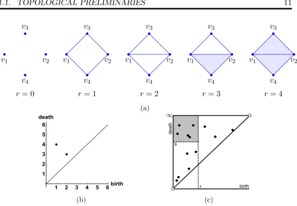
Figure 1.2: A filtration of simplicial complexes and its 1st persistence diagram in (a) and (b) respectively. In (c), the shaded area describes the relationship between persistent Betti numbers and persistence diagram.
Definition 1.10 (Tameness). The persistent homology Hk(K) is said to be tame if for all r ≥ 0, dim(Hk(Kr))< ∞ and the number of homological critical values is finite.
Since we consider the filtrations built on finite vertex sets, the assumption of tameness is always satisfied even if the index set is infinite. Let ∆ = {(x, y) ∈ R¯2: 0≤x < y≤ ∞}. Let for (x, y)∈∆, I(x, y) be an interval module, i.e., a family of vector spaces Ur alongwith linear maps Idr,s, where
Ur =
F, x≤r < y, 0, otherwise,
and Idr,s are the identity maps for x ≤ r ≤ s < y. Then under the assumption of tameness, we have the following isomorphism [71]
Hk(K)∼=
⊕p i=1
I(bi, di),
where the indices p ∈ N and (bi, di) ∈ ∆ for all i ∈ {0,1, . . . , p} are unique. Each summandI(bi, di) represents a generator of ak-dimensional hole which appears at bi
and disappears at di. We visualize this unique representation by the kth persistence diagram, defined as a multi-subset of ∆, i.e.,
Dgmk(K) ={(bi, di)∈∆ :i= 1,2. . . , p}.
12 1.1. TOPOLOGICAL PRELIMINARIES It may be possible that for somei̸=j ∈ {1,2, . . . , p},bi =bj anddi=dj, that’s why Dgmk(K) is a multi-set. As we shall see later, after introducing the randomness in the filtration, we identify Dgmk(K) as an integer-valued Radon measure rather than as a multi-set. Note that when k = 0, bi = 0 for all i in Dgm0(K). Let K be a filtration and its persistence diagram be denoted by Dgmk:= Dgmk(K). Then
βks,t(K) =|Dgmk([0, s]×(t,∞])|:=|{(bi, di)∈∆ : 0≤bi≤s≤t < di}|. (1.7) The above equation is illustrated in Figure1.2(c).
Example1.11. Let us summarize what is discussed so far with the help of the following example. Consider the filtration in Figure1.2(a). Letc1 =⟨v1, v3⟩+⟨v3, v2⟩+⟨v2, v1⟩ and c2 =⟨v1, v2⟩+⟨v2, v4⟩+⟨v4, v1⟩. Then the first 1-dimensional hole (or cycle) is generated byc1+c2, which appears at r = 1 and disappears at r = 4. The second 1-dimensional hole is generated by c2, which appears at r = 2 and disappears at r= 3. Note that the death times of the two holes will not be clear by simply looking at the figure and one has to calculate algebraically. Thus, we get (1,4) and (2,3) as the elements of 1st persistence diagram of the filtration, which is visualized in Figure1.2(b).
As in the case of usual Betti numbers, we again need some local structure to estimate persistent Betti numbers in the random setting. It turns out that they can also be estimated via simplex counts, thanks to Hiraoka et al. [30].
Lemma 1.12 ([30, cf. Lemma 2.11]). Let K={Kr}r≥0 and K˜ ={K˜r}r≥0 be filtra- tions of simplicial complexes such that for allr≥0,K˜r⊂ Kr. Assume thatKand K˜ are either ˇCech or Rips filtrations. Then
βks,t(K)−βks,t( ˜K)≤
k+1∑
j=k
(Sj(Kt)−Sj( ˜Kt)) .
Note that for general filtrations of simplicial complexes in Lemma 1.12, an ad- ditional term is required on the right hand side of the above inequality to hold (see Lemma 2.11 in [30]).
Remark 1.13. We remark that persistent homology defined here is a special case of a more general concept known as persistence module, defined for a sequence of general vector spaces [16].
1.1.3 Homotopy equivalence
In this subsection, we briefly describe the notion of homotopy equivalence. Let X and Y be two topological spaces and f0, f1: X → Y be two continuous functions.
A homotopy between the functions f0 and f1 from X toY is a continuous function H: [0,1]×X 7→Y such that for all x∈X,H(0, x) =f0(x) and H(1, x) =f1(x). In this case, we sayf0 andf1 arehomotopic and denote this byf0 ≃f1.
Definition 1.14 (Homotopy equivalent spaces). The topological spaces X and Y are said to be homotopy equivalent or of the same homotopy type (denoted by X ≃ Y) if there exist continuous functions g: X → Y and h: Y → X such that h◦g≃IdX andg◦h≃IdY, where IdX:X→X and IdY :Y →Y are identity maps.
Intuitively, two spaces are homotopy equivalent if the one space can be continu- ously deformed into the other space. For instance, a ballB(a, r) in RN or the whole spaceRN is homotopy equivalent to a pointp inRN. In both the cases, we can take H(t, x) = tp+ (1−t)x. We call such spaces, which are homotopy equivalent to a single point,contractible. Note that ifXandY are homeomorphic then they have the same homotopy type but the converse does not hold as can be seen from the above examples. For our purposes, we need the following fact: if a general topological space X is homotopy equivalent to a simplicial complex K, i.e,X ≃ K, then for anyk≥0, thekth singular homology group of X is isomorphic to the kth simplicial homology group of K [27, cf. Theorem 2.10 and Corollary 2.11]. We will use this fact in the next subsection.
1.1.4 Geometric complexes
In this subsection, we concentrate on a typical class of simplicial complexes, known as geometric complexes. Ageometric complex is a simplicial complex in which a subset of the vertex set is a simplex if and only if it satisfies some geometric constraint. So a notion of distance function is required to define the geometric constraint. Let (A, ρ) be a metric space from which we take the vertex set and construct simplices based on a constraint that is described using the metric ρ. We always deal with the following cases: (i)A ⊂RN withLebN(A)>0 andρis either aN-dimensional Euclidean met- ric or a general metric that can be locally approximated by a translational invariant metric induced from a weighted N-dimensional Euclidean norm and that is locally comparable to the Euclidean norm; (ii) Ais a compact m-dimensional manifold em- bedded inRN, wherem < N, and ρis aN-dimensional Euclidean metric; (iii) (A, ρ) is a compact m-dimensional Riemannian manifold. The motivation to consider the general metric in case (i) will be discussed in Chapter3. In this thesis, we work with the two well-known geometric complexes, known as ˇCech complexes and Vietoris-Rips complexes.
We first focus on the ˇCech complex. The construction of ˇCech complexes was first introduced by Alexandroff [1] and ˇCech [66] seprately. It has also received significant interest in TDA due to De Silva and Carlsson [18]. Let the closed ball of radius r and centered at x in the metric space (A, ρ) be denoted by Bρ(x, r), i.e., Bρ(x, r) = {y∈ A:ρ(x, y)≤r}. The ˇCech complex is defined as follows:
Definition 1.15(Cech complex).ˇ For a finite set of pointsX ={x1, x2, . . . , xn} ⊂
14 1.1. TOPOLOGICAL PRELIMINARIES A, theCech complexˇ with vertex set X and of radius r >0 is defined as
C(X, r, ρ) = {
∅ ̸=σ ⊂ X: ∩
x∈σ
Bρ(x, r)̸=∅ }
.
When r = 0, C(X, r, ρ) = X. Generally, the dimension of a ˇCech complex (as a simplicial complex) is very large as compared to that of A (as discussed in Sec- tion 1.1.1). However, the following theorem, known as the nerve theorem, due to Borsuk [13], says that if the metricρis nice enough then the kth homology groups of C(X, r, ρ) are trivial for all ‘higher’ values of k.
Theorem 1.16(Nerve theorem [13]). LetX be a finite set of points inA. Assume that for all subsets Y of X, the intersections ∩x∈YBρ(x, r) are either empty or con- tractible. ThenC(X, r, ρ)is homotopy equivalent to the union of balls∪x∈XBρ(x, r) =:
U(X, r, ρ), i.e.,
C(X, r, ρ)≃ U(X, r, ρ).
The assumption of the intersections to be either empty or contractible in Theo- rem1.16depends on the metricρ. Whenρ is aN-dimensional Euclidean metric, the balls are convex and so the assumption is satisfied. When ρ is Riemannian metric, there exists theradius of convexity rconv>0, which is the largest value of radiirsuch that every ball of radius r in Riemannian manifold is convex [12, p. 22] and hence, Theorem 1.16 holds for all r < rconv. It follows from Theorem 1.16 and the fact discussed in Subsection1.1.3that the simplicial homologyHk(C(X, r, ρ)) ofC(X, r, ρ) is isomorphic to the singular homologyHk(U(X, r, ρ)) of U(X, r, ρ), and so
βk(C(X, r, ρ)) =βk(U(X, r, ρ))
for allk≥0. Whenρ is theN-dimensional Euclidean metric in either case (i) or case (ii),U(X, r, ρ)⊂RN and dim(U(X, r, ρ)) =N for allr >0. Therefore, using the fact (ii) from Subsection1.1.1, βk(C(X, r, ρ)) = 0 for allk ≥N. When ρ is Riemannian metric, dim(U(X, r, ρ)) =m for allr >0, wherem is the dimensional of Riemannian manifold and therefore, using the fact (i) from Subsection 1.1.1, βk(C(X, r, ρ)) = 0 for allk≥m+ 1 and for all r < rconv.
We now focus on the other geometric complex, known as Vietoris-Rips complex, for which we cannot have such a nerve theorem. Vietoris used this complex to define a cohomology theory for metric spaces [67], while Rips used this complex to study hyperbolic groups [26]. The definition of Vietoris-Rips complex is as follows:
Definition 1.17 (Vietoris-Rips complex). For a finite set of pointsX ={x1, x2, . . . , xn} ⊂ A, the Vietoris-Rips complex with vertex set X and of radius r > 0 is defined as
VR(X, r, ρ) ={∅ ̸=σ ⊂ X:ρ(xi, xj)≤2r for all xi, xj ∈σ withi̸=j}.
Whenever ρ is a Euclidean metric, we remove the symbol ρ from the notations of the two complexes and Euclidean ball. When X ⊂RN and ρ is a N-dimensional Euclidean metric, the two complexes are related by the following chain of inclusions
VR(X, r′)⊂ C(X, r)⊂ VR(X, r), for all r′ ≥r
√ 2N N + 1.
The second inclusion follows directly from the definitions of the two complexes, and indeed, it holds in general, i.e.,C(X, r, ρ)⊂ VR(X, r, ρ). The first inclusion is proved in [61, Theorem 2.5]. There are also cases when the two complexes coincide. For instance, whenX ⊂RN andρ(x, y) = maxi∈{1,...,N}|xi−yi|,C(X, r, ρ) =VR(X, r, ρ).
We conclude this subsection with the reasoning that it is not possible to have a analogue of the nerve theorem for Rips complexes. We show this in R2 that can be easily generalized to RN. Let X be 2k+ 2 points equi-distributed on a circle of diameter r +ε. Then the Vietoris-Rips complex of radius r constructed on these 2k+ 2 points is isomorphic to the boundary of a (k+ 1)-dimensional cross-polytope, which is homeomorphic to ak-dimensional sphereSk. Therefore,Hk(VR(X, r))̸= 0.
By a (k+ 1)-dimensionalcross-polytope, we mean the convex hull of the 2k+ 2 points {±ei}, wheree1, e2, . . . , ek+1 are the standard basis ofRk+1. This reasoning is taken from [61]. See [61, Figure 1] for an intuitive explanation.
1.1.5 Critical points
We have stated in Section 1.1.1that dealing directly with Betti numbers in random setting is difficult and using simplex counts, which are the local phenomena, to esti- mate Betti numbers is one way to overcome this difficulty. On the other hand, there are another local structures known as the critical points of a distance function that also have connections with Betti numbers (of related ˇCech complexes) via Morse the- ory. This direction of research is mostly carried out by Bobrowski and his co-authors in several papers [7,10,12,11]. In this subsection, we give a brief introduction of the critical points and their relation with Betti numbers in the deterministic setting.
Let X be a finite subset of RN. Let distX:RN → R+ be the distance function which measures Euclidean distance to the setX, i.e.,
distX(u) = min
x∈X∥x−u∥.
Note that since distX is not everywhere differentiable, classical Morse theory can not be applied directly. However, via the results in [24], Bobrowski and Adler in [7]
pointed out that whenX is finite, one can still define the notion of critical points for distX and their Morse index, by which information about the Betti numbers of related Cech complexes (i.e., having vertex setˇ X) can be deduced. To have connections between the critical points of distX, which will be defined soon, and Betti numbers of the related ˇCech complexes, we need the assumption that the finite set X is in general position, which means the following: