Naturalness learning and its application to thesynthesis of handwritten characters

(1)

九州大学学術情報リポジトリ

Kyushu University Institutional Repository

Naturalness learning and its application to the synthesis of handwritten characters

Dolinsky, Jan

https://doi.org/10.15017/460987

出版情報：Kyushu University, 2008, 博士（工学）, 課程博士バージョン：

権利関係：

(2)

Dissertation 2008/2009

Naturalness Learning

and Its Application to the Synthesis of Handwritten Characters

ê6UfÒh]nÜ(kKøMW

December 17, 2008

J´ an Dolinsk´ y

Kyushu University

(3)

Abstract

The modeling of human-like behaviour has recently become important in various fields of engineering. Naturalness is defined in this study as the difference between target human-like behaviour and the behaviour of an original basic system which resembles the desired target human-like behaviour but lacks human idiosyncrasy. The added value contributed by naturalness is easily understood by comparing the following: Motion trajectories of industrial robots vs. those of AIBO robots; motions in technical simulations vs.

those of computer generated humans in games and movies; understandable synthesized speech vs. emotional speech; technically correct musical perfor- mances that follow the score vs. those performed by an expressive musician;

letters based on font shapes vs. handwriting.

All the above examples can be understood as cases where naturalness is added to a basic system. In the handwriting example, the basic system is comprised of the strokes of an original font character and the naturalness of the differences between handwritten strokes and the original font strokes.

If it is possible to generate the appropriate differences (naturalness) for the strokes in the font characters, then simple addition of the naturalness to the font strokes would yield handwritten characters. An intriguing question raised by the use of such an approach is: How is the naturalness related to the font strokes which represent the basic system? Additionally, is it possible to generate the right sort of naturalness? This doctoral thesis tries to provide the answers to these questions by mathematically analyzing the relationship between the font and its naturalness using canonical correlation analysis, multiple linear regression analysis, feed-forward neural networks (FFNN) with sliding windows, and recurrent neural networks (RNN). It also attempts to show that certain systems can be viewed in terms of a naturalness learning framework.

(4)

Ö

Ö Ö ¹ ¹ ¹n n n è è è

ºnFj/DþYSho.åfÎgÍkjc fMfD ê6UkþYØ ¡$oHpåm(íÜÃÈn Õ\ÌáhAIBOnÕM S·ßåìü·çóh²üà ;nº

CGnÕ\ãïýjóðhhÅJKjóð }\kcº!Ô jOhhÅJKjOÕ©óÈkKhKøMnK ji

ÔYp¹kãgMF

SºWD/Doú,·¹Æàkê6U H_nh WfâÇëgM KøMn4ú,·¹ÆàoÕ©óÈgB

ê6UoKøMhÕ©óÈhnºìkøSY ºn/, O, ø

;InâÇëú,·¹Æà \W SnâÇëKU

_Õ\OWh nºn/OIhnîê6U gBhîY ]ng (1) âÇëKSnê6UfÒY

âÇëÐHW, (2) Snê6UnâÇëKøMWnê6UfÒk

Ü(W, (3) KøMWnê6UnfÒ.âÇëgfÒWfãW

(4) KøMWnê6UnfÒkrecurrent neural networks (RNN)(D f RNN nê6UfÒ'ýnkdDfkÔßY

î·¹Æàn/toú,·¹Æàn/bhê6Unh nD sgn Õ* Õ£ Õ+hDFs ghþU

t =b⊕n nhH ,Ögo!nîê6UhW ffÒþahW fÒU_ê6Uú,·¹ÆàkX YâÇ ët =b+n gî·¹Æàn/Y Hpºn Oo}\nwUkê6U³YShghþgMhDFî¬âÇëg BSnâÇëoDDjÕ\kÜ(gML,Ögo º

nKøMWî·¹Æàn/ hÕ©óÈú,·¹Æàn/

nîê6UhWffÒW fÒW_ê6UÕ©óÈk Y

ShgKøMWLF

KøMWnÐHâÇënw@ndo t = b+w×n (_`

W0 ≺w ≺1)hê6UkÍØQYShg ê6U¦DDj

¿tgMKøMWLïýkj¹gB Sn¹LF(nKø MÕ©óÈ\½ÕÈh'MOpj ÍL1n4oKøM,ºn

Wk^8kÑDKøMWLU HpÍL0.6n4o Õ©óÈK60% ]nKøM,ºnWkÑeD_KøMWL U Í0oÕ©óÈW]nnYShkj

Õ©óÈ¹Èíü¯Å1Õ©óÈn¹g:W_#Ym¹Ù¯

ÈëghþY Snm¹Ù¯ÈënÕ©óÈ¹Èíü¯Å1eh

(5)

W Õ©óÈn¹hþÜYKøMWn¹hnîÙ¯Èëm¹

úYFfÒYShH Snem¹húm¹n¢Â

cø¢gãYh eúLÚbkÑDWBc_L OnWgoeLhþgMúnê6UoZK30% ¦WKj Kc_ SnPKem¹Ù¯ÈëghþW_Õ©óÈ¹È íü¯Å1 húÕ©óÈhKøMWhnî n¢Âo^

ÚbgBFh¨ßU

]Sgfeed-forward neural networksFFNN FFNN with sliding

windown^ÚbâÇë cfeúy'nfÒLDãW_

nPíB¶neLÅgBShoKc_L FFNN

with sliding windowgAkSneú¢ÂfÒgMjDShL

Kc_SnPKôkattractorâÇêó°nÅ'k@îWRNN

koecho-stateØMRNN)( eWffÒW_hS eú

y'nâÇêó°LF~OúeFkjc_ Uk9o Hú

dæËÃÈgnêñÕ£üÉÐÃ¯ROL eYRNNâÇë

HW 'ýØShLgM_

,vnPKÕ©óÈWehW Õ©óÈWhKø MWhnîÙ¯ÈëúhYê6UnfÒko ^ÚbfÒK ÕLï gBRNN ykROLeYShg'ý(k ØShLgMSh:W_ Ukê6UfÒnÜ(hWf Õ©óÈWkNNúnê6UÍØQ YShgKøMW

W U¡W_

(6)

Handwriting is a dialogue between the writer and his inner voice, where ideas organically take on shapes that reflect his original thoughts. Reading handwriting opens a dialogue with the writer, and a window not only into his original thoughts, but also his feelings and intentions.

Handwriting, therefore, makes communication more valuable for both, reader and writer, and can not be replaced by a computer.

If this work only serves to remind us of the inherent value of handwritten communication then my goal will be achieved.

(7)

KøMgøOhDFShoøMKhøMKnÃnþqgB Kø MhDFShoøMKhnþqgB øMKnÃ~gngB

]nKoøMKLH_DSh`QgojO øMKnÅ hÿâLH

W_LcfKøMnWoøMKhKn³ßåË±ü·çó nê RShogMSnFj³ßåË±ü·çóo ³ó Ôåü¿ügþYShogMjD

KøMnWny j¡$XU[ShL Ánîn dg B

(8)

Chapter 1 Introduction

1.1 Background and Remained Problems

The modeling of handwriting and other human-like behaviour is becoming increasingly important in various fields of engineering. Naturalness in this study is defined as the difference between target human-like behaviour and the behaviour of an original basic system which resembles the desired target human-like behaviour but lacks human idiosyncrasy. It is easy to understand the added value that naturalness provides by looking at a few real-world applications — compare the motion trajectories of industrial robots to those of AIBO robots, which provoke an emotional response in their users; the motions of objects in technical simulations to those of computer generated humans in games and movies; comprehensible synthesized speech to emotional speech; a musical score played back automatically with technical perfection to music played with nuance by an actual musician; or letters based on font shapes to handwriting.

The above examples can be understood as cases where naturalness is added to a basic system. In the handwriting example, the basic system is comprised of the strokes of an original font character and the naturalness of

(12)

the differences between handwritten strokes and their corresponding original font strokes. If it were possible to generate appropriate naturalness (difference) for the strokes of a font character, then synthesizing a handwritten character would be reduced to the simple addition of the naturalness to the original font strokes. This study analyzes the relationship between certain properties of font strokes and their naturalness. Obtained results show that it is also possible to generate appropriate naturalness for characters which were not introduced during the training stage.

The way we write is deeply individual [1], and handwriting is therefore preferable in certain situations where this personal touch makes communication more valuable. Synthesizing handwritten characters enables us to create a font that automatically reflects a person’s writing style; when this font is then used to communicate (e.g. by email, instant messengering, etc.), it implies a closer relationship with the recipient. As a result, the recipient of a message written using a personalized font may be inclined to feel more warmth towards the sender. The need for warmth and emotions is particularly obvious in text-to-speech synthesis [2, 3].

Although synthesis of handwritten characters has been studied in many previous works [4, 5, 6, 7, 8, 9, 10, 11, 12], a transparent and easy-to-use synthesizing technique is still lacking. The synthesis of handwritten letters often involves complicated template point matching [8], feature correspondence between training samples [10] or requires to provide several allographs per each character [7, 11]. The lack of a simple technique is a reason why a system for on-line synthesis of handwritten characters has not yet been implemented in any major operating system. Creating a personalized font is only a half-solution because personalized font does not change once created.

It is therefore desirable that a system for on-line synthesis of handwritten

(13)

characters would turn existing font characters into handwritten forms on the fly while typing on a keyboard with shapes of the same letters being always slightly different. Using fonts which are already available in computer makes an implementation of such a framework considerably easier and might result in its widespread use.

1.2 Objectives and Approaches

This study serves to improve our understanding of human-like behaviour, by using handwriting as an example. Hopefully, synthesized handwritten letters, in for example email communication, will demonstrate the irreplaceable value of handwritten communication and revive the lost art of handwriting;

something that can not be replaced by computer.

The objective of this study is to provide a transparent and easy-to-use technique for modeling human-like behaviour. Feasibility of the proposed naturalness learning is examined by applying the naturalness learning to the handwriting task where handwritten characters are synthesized by means of adding generated naturalness to the original font strokes. The key point of this study is therefore a question as to whether a relationship between the font strokes and their naturalness exists, and furthermore, whether it is possible to generate appropriate naturalness for the font characters which were not included in a training set.

The relationship between certain properties of the font strokes and their naturalness is analyzed with emphasis on generating the right sort of naturalness for characters that were not introduced during a training stage. The analysis is carried out using various linear and nonlinear techniques. At- tempts to analyze this relationship using linear techniques such as canonical correlation analysis [13, 14] and linear regression [15] are followed by trials

(14)

using nonlinear techniques including feed-forward neural networks (FFNN) [16], FFNN with sliding window and recurrent neural networks (RNN) such as RNN with echo-states [17, 18]. All trials were carried out with a training set made of selected hiragana letters. Once an appropriate technique was found, we also attempted to model naturalness for letters that were not included in the training set.

In the following chapters, we use termcharacterrather then letteras it is more general term. Although, the symbols of japanese syllabary Hiragana, used thorough the dissertation, represents sounds only, and thus, they can be referred to as letters.

A glyph is an element of writing. Two or more glyphs representing the same symbol, whether interchangeable or context-dependent, are called allographs; the abstract unit they are variants of is called a grapheme or character. Glyphs may also be ligatures, that is, compound characters, or diacritics [19].

1.3 Structure of This Dissertation

This dissertation is organized as follows: Research related to this study and related modeling techniques are discussed in Chapter 2. Naturalness learning framework is explained in detail in Chapter 3. Chapter 4 provides details regarding how to extract naturalness and input signals from font strokes.

Analysis of the relation of the naturalness and the input signals using various linear and nonlinear techniques is provided in Chapter 5. Chapter 6 gives further mathematical analysis on the dynamics of RNN with recurrent output layer - a technique that was found to perform the best. Discussions concerning mathematical and philosophical aspects of this study are given in Chapter 7. Finally, the study is concluded in Chapter 8 where obtained

(15)

results are summarized and new prospective applications for the naturalness learning framework are outlined. The overall structure of this dissertation is shown in Fig. 1.1

Figure 1.1: Structure of this dissertation.

(16)

Chapter 2 Related Research and Techniques

2.1 Related Research

Naturalness in handwriting is often attributed to the idiosyncrasies of the action of writing. The hypothesis that the way we write is deeply individual relies solely on subjective observations. Srihari uses a subset of attributes used by forensic document examiners to quantitatively establish individu- ality in handwriting through machine learning techniques [1]. The method determines the identity of the writer, with a high degree of confidence, by using global attributes of handwriting¹ and very few characters in the writing.

The study provides valuable information regarding factors that contribute to handwriting style.

The synthesis of handwriting has been addressed in many previous works.

Generative techniques can be divided into two categories: movement simulation techniques [4, 5, 6, 20] and shape simulation methods [7, 8, 9, 10, 11, 12].

Movement simulation techniques are mostly derived from the kinematic

1Attributes which belongs to an entire document structure; i.e. slope of lines, distance between paragraphs, etc..

(17)

theory of human movements [21]. Bullock uses a neural network model, called VITEWRITE model, to generate complex curvilinear handwriting movements [20]. A sequential controller, or motor program, interacts with a trajectory generator to move a hand with redundant degrees of freedom. The vector integration to endpoint (VITE) model for synchronous variable-speed control of multi-join movements serves as the neural trajectory generator.

VITE model enables a simple control strategy to generate complex curvilinear handwriting if the hand model contains redundant degrees of freedom.

Modeling handwriting with movement simulation techniques often implies a dynamic-inverse problem, which is difficult to solve [6].

In contrast, shape simulation techniques concentrate on the trajectories of the handwritten strokes, which already embody the characteristics of an individual’s personal writing style directly in their shapes.

Wang J. provides a comprehensive mathematical analysis of cursive roman handwriting [8]. The writing style of a specific character is represented as a distribution of sparse sequence of control points that define the character, where the distribution parameters are estimated from several allographs.

A deformable energy model is used to concatenate adjacent letters.

Contrary to Wang J., where a character is represented by several control points only, Lin uses dense sequence of control points to represent a character glyph [11]. All individual characters that appear on QWERTY keyboard are required to be written three times (94 characters in total) via the system’s user interface for collecting user handwriting samples. The three allographs for each character serve for glyph variation. During the synthesis, one allograph per each character is sampled according to the system’s rules and additional shape variation is added using geometric deformations. Generated glyphs are aligned so that words are composed with proper horizontal inter-

(18)

character space and vertical offset being taken into account. Probability of connecting adjacent glyphs is estimated and ligatures between neighboring glyphs are generated according to the estimated probability. The system particularly respects the cursiveness so that a user can choose the cursiveness that varies from completely hand-print to completely cursive.

Choi uses an online handwriting recognizer based on a Bayesian network to generate the most probable points for a character on a 2-D plane [9]. The system generates average character shapes using training samples from many different writers.

All three approaches [8, 9, 11] require that, in order to synthesize a given letter e.g. A, the system must be trained on that letter; to synthesize an entire alphabet, all characters from that alphabet must be used in training.

Wang L. generates calligraphy by computing intermediate allograph C_t using two sample allographs C₀, C₁ where parameter t ∈ [0,1] represents a tendency to mimic either C0 orC1 [7]. Outlines of strokes are represented by the deformable contourg-snakemodel. The intermediate allographCtis generated by adjusting g-snake control parameters of each stroke. The g-snake control parameters are computed from the corresponding pair of strokes in the two sample allographs using regularization. This simple, yet sophisti- cated, approach works well with Japanese hiragana and roman alphabet. To generate a given letter e.g. A, two different allographs of A (C₀, C₁) have to be provided.

Xu generates artistic Chinese calligraphy using a constraint-based Analogous- Reasoning Process (ARP) [10]. Their proposed system is essentially a specific version of a deformable model. Hierarchical representation of complex Chi- nese characters is the basis of this approach. The ARP synthesizes new knowledge (shapes in this case) by fusing or blending existing knowledge

(19)

sources (shapes from training samples). Typically, fewer than 10 samples for each character suffice for generating new calligraphy art. Required samples for each character may be provided from different fonts and are not neces- sarily required to be in a handwritten form. The system is able to reflect user’s style even from a few handwritten samples if the user’s handwriting is not too peculiar so that it lies outside the feasible space composed from the provided fonts.

A mention should be also made to the Loeb’s patent which addresses the synthesis of handwriting with personalized fonts [12]. It had been only recently published and due to time restrictions a thorough investigation was not possible.

The approach we introduce in this study is a shape simulation technique.

It is similar to [10] in that the deviation by which the canonical reference shape (i.e. font) and a training sample shape differ is used when fusing a new shape. The substantial difference is that our approach is concerned with modeling of those deviations, whereas [10] models weights (ARP intensities), which control the contribution of the i-th training sample deviation to the overall result. The representation of the deviations is also different, and our approach does not require complicated feature correspondence between training samples.

Despite a thorough search, we could not find any other works where the target human-like behaviour is modeled by means of combining the naturalness with the original basic system or where the naturalness is defined as the difference between the target human-like behaviour and the behaviour of an original basic system. Preliminary results were first published by the author and his supervisor in [22].

Much work has been done on improving naturalness in text-to-speech

(20)

synthesis [23, 24, 25, 26]. These studies, however, use comparative quality tests where listeners rank naturalness of synthesized speech and are not related to the approach presented here. Improving naturalness in text-to- speech synthesis is achieved by by improving the prosody rules according to the obtained rank. The approach presented in this study achieves the target human-like behaviour by adding naturalness to the behaviour generated by the basic system whereas their approach improves the basic system directly by improving the prosody rules.

Generation of human movements is yet another challenging task which has been the subject of many previous studies. It is out of the scope of this study to provide comprehensive overview regarding numerous algorithms for generation of human movements (inverse-kinematics algorithms, etc.).

Already established movement simulation techniques might be able to serve as a basic system for generating natural human movements with naturalness learning framework. Studies concerning congruity between perception and data of human movements [27] however suggest that adding naturalness to motion generated by such a system is by no means straightforward.

2.2 Related Techniques

2.2.1 Cubic B´ ezier Curves

In vector graphics, B´ezier curves are an important tool used to model smooth curves [28]. Combinations of B´ezier curves patched together are often called paths. In image manipulation programs such as Inkscape, Adobe Illustrator, Adobe Photoshop, and GIMP paths are used to create complex curve shapes.

B´ezier curves make sense for any degree. This section describes the cubic ones, which are the most important. A cubic B´ezier curve is specified

(21)

by four points, called control points. Mathematically, the B´ezier curve is just a particular linear combination of the control points with time-varying coefficients. Control points P₀, P₁, P₂, P₃ would yield a curve given by

P(t) = (1−t)³P0+ 3(1−t)²tP1+ 3(1−t)t²P2+t3P3

t∈[0,1]

The time-varying coefficients arise from a binomial expansion of 3rd degree, hence the name cubic B´ezier curves. Recalling that (s+t)³ = s³ + 3s²t+ 3st²+t³, putting (1−t) for s and considering expanded terms individually rather than added together yields four functions of t, called the Bernstein polynomials.

B_0,3(t) = (1−t)³ = 1(1−t)³t⁰ B_1,3(t) = 3(1−t)²t= 3(1−t)²t¹ B_2,3(t) = 3(1−t)t² = 3(1−t)¹t² B_3,3(t) =t³ = 1(1−t)⁰t³

Thus a cubic B´ezier curve can be described by

P(t) =B_0,3(t)P₀+B_1,3(t)P₁ +B_2,3(t)P₂+B_3,3(t)P₃ t∈[0,1]

Bernstein polynomials and B´ezier curves can be defined for any degree n by using the expansion of (s+t)ⁿ. The general form for a B´ezier curve of n-th degree is given by

P(t) =

n

X

i=0

P_iB_i,n(t); t∈[0,1]

where P_i is a control point and B_i,n(t) is a Bernstein polynomial. The case where n= 3 is described since that is most frequently used.

(22)

Example. Let’s have four control points

P₀ = (6,12), P₁ = (15,15), P₂ = (6,2),and P₃ = (1,3). Then, P(t) = B_0,3(t)P₀+B_1,3(t)P₁+B_2,3(t)P₂+B_3,3(t)P₃

= (1−t)³(6,12) + 3(1−t)²t(15,15) + 3(1−t)t²(6,2) +t³(1,3)

= (6 + 27t−54t²+ 22t³,12 + 9t−48t²+ 30t³).

In other words, P(t) = (x(t), y(t)) with x(t) = 6 + 27t−54t² + 22t³ and y(t) = 12 + 9t−48t² + 30t³. The curve with its control points is shown in Fig.2.1.

P₀

P₁

P₃

P₂

Figure 2.1: Example of a cubic B´ezier curve.

2.2.2 Multiple Linear Regression Analysis

Relation between a variable of interest (the response) and a set of related predictor variables can be investigated and modeled by a regression analysis.

Contribution of each predictor variable x_i to the response variable y can be expressed as follows.

y =β₀+β₁x₁+β₂x₂+· · ·+β_kx_k+ε

The parameters β_j, j = 0, . . . , k, are called the regression coefficients or the model parameters with ε being a random error component. Customarily x_i are called the independent variables and y is called the dependent variable.

(23)

This terminology, however, might cause confusion with the concept of statis- tical independence, and thus,x_i is referred to as the predictor or the regressor variables and y as the response variable.

The above equation is called multiple linear regression model because it involves more than one regressor variable. The term ’linear’ stems from a fact that the equation is linear function of the unknown parametersβi, even though the relationship between y and xi may be expressed in a nonlinear fashion (f.e. linear model with polynomial terms).

Sample regression model corresponding to the above equation may be written as

y_i =β₀+β₁x_i1+β₂x_i2 +· · ·+β_kx_ik+ε_i i= 1,2, . . . , n and may be further expressed in matrix notation

y=Xβ+ε

whereyis a n×1 vector of the observations,Xis ann×k+ 1 matrix of the regressor variables, β is a k+ 1×1 vector of the regression coefficients, and ε is an n×1 vector of random errors. The objective of regression analysis is to find the vector of least-squares estimators, ˆβ, so that

S(β) =

n

X

i=1

ε²_i =ε⁰ε= (y−Xβ)⁰(y−Xβ) is minimized. S(β) may be also written as

S(β) = y⁰y−β⁰X⁰y−y⁰Xβ+β⁰X⁰Xβ

=y⁰y−2β⁰X⁰y+β⁰X⁰Xβ

(24)

Global minimum of S(β) can be found by computing βwhen a derivative of S(β) is equal to 0.

∂S

∂β =−2X⁰y+ 2X⁰Xβˆ which simplifies to

X⁰Xβˆ =X⁰y resulting in the least-squares estimator of β being

βˆ = (X⁰X)⁻¹X⁰y

Estimation of the unknown model parameters is also known as fitting the model to the data and can be done using various techniques with the least-squares method being the most commonly used. After the estimation of the model parameters, model adequacy checking has to be carried out in order to determine the appropriateness and the quality of the fit [15].

2.2.3 Canonical Correlation Analysis

Multiple linear regression analysis is a multivariate technique, which can estimate a value of a single response variable from a linear combination of a set of predictor variables. For some research problems, however, researcher may be interested in relationship between sets of multiple predictor and multiple response variables, rather than single response variable only. The linear relationship between two sets of multiple variables can be investigated using Canonical correlation analysis (CCA), first proposed by Hotelling [13] and further developed by Anderson [14].

Let’s havenpairs of observed vectors (x_i, y_i), eachx_i being ap-vector and each y_i being a q-vector. Let V₁₁ and V₂₂ be the sample variance matrices

(25)

for the observationsx_iandy_i, respectively. WriteV₁₂for thep×qcovariance matrix between the x_i and the y_i,

V₁₂ = 1 n−1

n

X

i=1

(x_i−x)(y¯ _i−y)¯ ⁰ and let V₂₁=V⁰₁₂ [29].

CCA computes p-vector a and q-vector b so that linear combinations a⁰xi and b⁰yi are as highly correlated as possible. In other words, original multivariate observations xi and yi are reduced into univariate linear compoundsa⁰x_i andb⁰y_i. The univariate linear compoundsa⁰x_iandb⁰y_iare called canonical variates and the vectorsaand bare called canonical variate weight vectors.

The computation of the vectorsaandbcan be expressed as an eigenvalue problem. Note that the sample variances of a⁰x_i and b⁰y_i are a⁰V₁₁a and b⁰V₂₂b. Similarly, the sample covariance of the pairs (a⁰x_i, b⁰y_i) is a⁰V₁₂b.

Computation of the canonical variate weight vectors can be expressed as the optimization problem

max a⁰V₁₂b subject to a⁰V₁₁a=b⁰V₂₂b = 1

It can be shown that this problem can be solved by computing eigenvalue ρand corresponding eigenvector

a b

of the generalized eigenvalue problem.

0 V₁₂ V12 0

a b

=ρ

V₁₁ 0 0 V22

a b

Computed value of ρ is the correlation between the variates a⁰x_i and b⁰y_i. Solving the equation completely gives the r = rank(V₁₂) ≤ min(p, q) strictly positive eigenvalues ρ₁ ≥ ... ≥ ρ_r and corresponding eigenvectors (a₁, b₁), ...,(a_r, b_r) [29].

(26)

Squared canonical correlations (canonical roots) provide an estimate of the shared variance between the canonical variates but provide no information concerning how much variability in the original sets is explained by their respective canonical variates. It is often the case that strong canonical correlation is obtained between two linear composites (canonical variates), even though these linear composites does not extract significant portions of variance from their respective sets. To measure the amount of variance in one set of variables that can be explained by the variance in the other set, the Stewart-Love index of redundancy has been proposed [30]. To compute the amount of shared variance between the original sets and their respective canonical variates, the sum of squares of the correlations between the canonical variates and their original variables is divided by the number of original variables in the corresponding set. Recall that squared canonical correlation provides an estimate of the shared variance between the canonical variates themselves. The redundancy index of a variate is then obtained by multiplying the shared variance between the variate and its original set with the squared canonical correlation.

Redundancy indices can be computed for both predictor variables set and response variables set. In practice, however, usually only redundancy index for canonical variate of the response variable set is interpreted. One should also note that canonical correlation is the same for both variates, whereas the redundancy index will most likely vary between the variates.

2.2.4 Artificial Neural Networks

An artificial neural network system (ANN) is an abstract mathematical model inspired by brain structures and mechanism. Although ANNs mimic certain aspects of brain, they are only mere simplification of real neural net-

(27)

works being oriented towards information-processing tasks. ANN information- processing systems are an important special cases of the classical complex information-processing systems found in the classical engineering and math- ematics literature. In fact, many tasks solved by an ANN can be often investigated and modeled by a nonlinear regression models or linear ones with nonlinear terms. Regression models, however, usually require deeper knowledge concerning a task being solved, whereas an ANN is a robust modeling tool, which works well with many tasks. Robustness is probably one of the main reasons why ANN have become so popular in engineering and conversely also the reason for its overuse.

2.2.5 Feed-forward Neural Networks

ANN with no cyclic connection is called feed-forward neural network (FFNN) and represents a mapping of an input vector to an output vector. FFNN system has a layered structure, which consists of input layer, several hidden layers and output layer. Every layer has processing units (neurons), which receive their input from units from preceding layer and send their output to units in successive layer (Fig.2.2). There are no connections within a layer, hence the name FFNN. Layers are connected to each other using weighted connections. These weights are adapted during training process so that an input vectors are mapped to corresponding output vector with high precision.

Perhaps the best known learning algorithm for adaptation of the weights is the back-propagation learning rule [31, 16].

2.2.6 Recurrent Neural Networks with Echo-states

An ANN, which has one or more cyclic connections (Fig.2.3) is called recurrent neural network (RNN). An RNN represents a dynamical system because

(28)

input layer hidden layers output layer

Figure 2.2: A two layer feed-forward neural network.

cyclic connections within the RNN makes output being influenced not only by an input vector but also by previous internal states of the network. This usually leads to highly nonlinear behavior of the network, what in turn allows to model complex systems. RNN is particularly useful for investigating and modeling of temporal patterns. Approximation capabilities of an RNN are not higher than that of a FFNN [16]. One might, however, obtain a solution with lower number of units or eliminate necessity for time-delay line, etc..

RNNs are in general difficult to train. There are several training algorithms with some of them being adaption of back-propagation rule to RNN.

Werbos explains in detail how to use the back-propagation rule with RNN [32]. Some difficulties with the training are highlighted in [33, 34]. Approach proposed by Jaeger eliminates many difficulties with the training of RNN by introducing echo-states; high dimensional expansions of input vectors where the expansion of the previous input vector is incorporated in the current expansion in a contractive fashion [17].

x(n+ 1) =f(Wⁱⁿu(n+ 1) +Wx(n))

(29)

Contractions of the expansion x(n) is guaranteed when biggest eigenvalue of the matrixWis less than 1. An output is computed right off the expansions as a weighted linear composite of the expansion components.

y(n+ 1) =f^out(W^outx(n+ 1))

There are various modifications to the above equations. Details concerning the generation of the input and internal weights Wⁱⁿ and Wwith a descrip- tion of the training algorithm are available in [17].

input layer internal units output layer

Figure 2.3: A recurrent neural network with two cyclic connections.

(30)

Chapter 3 Naturalness Learning Framework

3.1 Introduction

A generalized approach to naturalness learning is described first and then its principles are demonstrated by applying it to the handwriting task.

We begin by distinguishing between a target system and a basic system.

Target system refers to the system whose behavior we wish to model. The behavior of the target system is usually quite complex. By basic system, we refer to a system whose behavior is to be usedwhile modeling the target system. The use of the word basic is not intended to suggest anything about the complexity of the basic system; rather, by convention, basic systemis chosen because it implies that the system’s behavior is well described. Intuitively speaking, the target system resembles the basic system, except its behavior represents to some extent a deviation from the basic system. These deviations are referred to as naturalness. It is also assumed that this naturalness has some relationship with the basic system. The task of the naturalness learning is to find and learn this relationship.

Once the relationship is learned, the behaviour of the basic system and

(31)

generated naturalness can be combined in order to obtain the complex behavior of the target system. Thus, instead of modeling the behaviour of the target system directly, the difference (the naturalness) between the behaviour of the target and basic system is modeled. An important point here is that this approach enables us to control the amount of naturalness being added to the basic system; by weighting the naturalness with values from the interval [0,1], one can obtain a system with a given amount of naturalness. A weight with value 1 will render a system’s behavior as close to the target system as possible. A weight with value, e.g. 0.4, on the other hand, will reduce the naturalness to 40%, and a weight value of 0 will render the system’s behavior identical to the basic system.

3.2 Naturalness Learning for Handwritten Char- acters

The generation of handwritten characters is the task we chose to illustrate the application of the naturalness learning approach. In this study, the characters used are hiragana, symbols of the Japanese syllabary, with the ultimate intention being to synthesize Chinese characters. Hiragana evolved over the centuries as simplifications of certain Chinese characters and it is for this reason that we choose hiragana for our experiments.

Although everybody learns their alphabet at school, the way we eventu- ally write the characters of the alphabet is deeply individual. We can therefore understand handwriting as the transformation of the canonical shape of a character as learned in school into the writer’s individual handwritten form. Let’s refer to the characters as they are written in primary school textbooks as font characters, or fontC. Handwriting can then be considered the process of turning afontC into its handwritten form, or handC. In other

(32)

words, the naturalness, which is being added to fontC, resulting in a handwritten character, is a sort of personal ’discrepancy’ between the individual’s handwriting and the canonical form.

Speaking in terms of naturalness learning, the handwritten characters are the target system and the font characters are the basic system. The naturalness to be modeled is thus the difference between the handwritten characters and the corresponding characters of the font, and it reflects the individual- istic qualities of a person’s writing style because handwritten characters are specific to their writer. Essential to our ability to use this approach is the validity of our assumption that the naturalness is related to the basic system, the characters of the reference font.

Figure 3.1: Hiragana character /ka/. Naturalness expressed by a 2-D displacement vector field. Font character strokes are shown in black, handwritten strokes are shown in blue.

Naturalness can be expressed by any arbitrary mechanism. In this study, we express the naturalness as a 2-D displacement vector field between evenly spaced points along the strokes of the font and its corresponding handwritten version (Fig. 3.1). The 2-D displacement vector field serves as an output in the naturalness learning framework (Fig. 3.2). The font characters (the basic system) are described by certain properties computed at evenly spaced points

(33)

along the strokes of the font character and serve as an input in the naturalness learning framework. The input and output data are discussed in detail in the following chapters.

Figure 3.2: Naturalness learning framework, where 2-D d.v.f. = 2-D displacement vector field.

Because we are modeling the naturalness and not the actual target system, we are able to control the amount of the naturalness being added to the font characters (Fig. 3.3). A weight value of 1 will render generated characters as close to the person’s handwriting as possible. A value of, for example, 0.6 will reduce the naturalness to 60% providing us with neat handwritten characters. Values close to 0 (approaching 0 from right side) will render generated characters that are very close to the font characters.

The proposed naturalness learning approach is not limited to this handwriting task. Generating natural looking movements for parts of a human body, with inverse kinematics algorithms being employed as the basic system or generating emotional human speech with synthesized speech being used as a basic system are interesting and challenging applications of the naturalness learning approach.

(34)

Figure 3.3: Controling the amount of naturalness being added to the font character, wheresynthC= synthesized character andfontC= font character.

(35)

Chapter 4 Extracting Naturalness in Handwritten Characters

In this chapter we further develop the idea of naturalness learning and explain in detail how naturalness is extracted from handwritten characters. We also describe, which properties offontCstrokes were extracted. Naturalness plays the role of the output in the naturalness learning framework with fontC strokes being used as an input.

4.1 Extraction of Stroke Points

ThefontCwere extracted from the Bitstream Vera Sans font onto a 250×250 pixel canvas. Every stroke of each character was turned into a path comprised by a set of cubic B´ezier curves [28]. At this stage, an Open Source vector graphics editor (Inkscape) was used to manually extract strokes from the characters of the font. Every path was then evenly broken up into a set of points with a spacing interval ¹ of 8 pixels being used. Several other spacing intervals were also tested. Further discussion is available in Section 4.6. Let eachP^{f ont}_ij be a matrix representing the set of points n_ij×2 where idenotes

1an arc length between a pair of successive points

(36)

the index of the character, j is the index of the stroke within the character and n_ij its number of points. P^{f ont}_ij (k) = (x_k, y_k) represents thek-th point of the j-th stroke of the i-th character (the k-th row of the matrix P^{f ont}_ij ).

ThehandCwere first scanned, manually extracted using the Inkscape editor, and then appropriately scaled to ensure they fit the canvas. EveryhandC stroke was then aligned to its corresponding fontC stroke. This alignment ensures that the displacement vector field expresses only the shape transformation corresponding to the matching of the fontCand handC strokes. The same procedure as with fontC was again used to decompose the strokes of handC, with the points for each stroke being stored in the matrixP^hand_ij . The spacing interval along each stroke (path) of a handC was, however, adjusted so that it was comprised by the same number of points as its fontC stroke.

The process of stroke points extraction is shown in Fig.4.1.

4.2 Font Strokes: an Input

Many different signals were extracted from the strokes of fontC in order to find the most suitable input signals. When a person is about to write a character, he or she knows what the shape of the character is supposed to look like, and thus, tries to adjust his or her writing trajectory to match the shape of the original character. We want therefore to represent the strokes of fontC so that the extracted data represent the trajectories of the original character the person is going to write. Moreover, we want this representation to be position independent to ensure that the same stroke written in e.g. the lower left corner of the canvas and in upper right corner of canvas is represented by the same data. The difference vectors between all pairs of successive (evenly spaced) points along a stroke fulfill both requirements. They represents the trajectory of the original character and also offer a position-independent rep-

(37)

Figure 4.1: Data extraction work flow.

resentation. In the following, these vectors are referred to as inertiabecause they describe the tendency of an imaginary pen to follow the trajectory of the original character. Fig. 4.2 plots the difference vectors along strokes of font hiragana character /ra/.

The mathematical definitions of the input signals are as follows. Let D^{f ont}_ij (k) be the difference vectorP^{f ont}_ij (k+ 1)−P^{f ont}_ij (k). The inertia for the k-th point of thej-th stroke of the i-th letter is then given by

inertia_ij(k) = D^{f ont}_ij (k) (4.1) with eachinertia_ij(k) being thek-th row of the (n_ij−1)×2 matrixinertia_ij.

(38)

Figure 4.2: Inertia between pairs of successive (evenly spaced) points along a font stroke. Distance along a font stroke for every pair is 8 pixels. D^{f ont}_ij (k) = P^{f ont}_ij (k+ 1)−P^{f ont}_ij (k) = (dxk, dyk).

Fig. 4.2 illustrates the geometrical meaning of (4.1). The inertia was used as default input data and, unless stated otherwise, the input data matrix U_ij(k) is made of the inertia only.

U_ij(k) =inertia_ij(k) (4.2) The components of every vector U_ij(k) represent the lengths of the legs of a right triangle, so each column of each matrix Uij is scaled by the same global factor a to ensure the ratio between the legs is preserved. The factor a is computed as a global maximum of elements in all matrices U_ij, and the scaled matrices fit in the interval < −1,1 >. In the following, U_ij always refers to the scaled matrix.

(39)

4.3 Naturalness: an Output

Naturalness, which serves as the (2 dimensional) output signal, is represented by a 2-D displacement vector field. The 2-D displacement vector field for the j-th stroke of the i-th character is given by

V_ij =P^hand_ij −P^{f ont}_ij (4.3)

withV_ij,P^hand_ij andP^{f ont}_ij each beingn_ij×2 matrices. Fig. 3.1 illustrates the geometrical meaning of (4.3). The last row of every V_ij is dropped to ensure that each pair of V_ij,U_ij have the same length ofn_ij−1. The scaling factor b is computed as a global maximum of elements in all matrices V_ij. Each matrix Vij is scaled by this global factor b to fit in the interval <−1,1>.

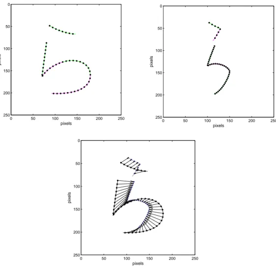
Fig. 4.3 shows actual process of aligning and computing 2-D displacement vector fields (naturalness) for the strokes of example character /ra/ with Fig. 4.4 showing the input and the output signals for an example character /ra/ prior to the normalization.

4.4 Additional Input Signals

Besides the default input data (inertia), some other signals were tested also.

A sine of the angleφ (Fig.4.2) is referred to as curvature. The curvature for the k-th point of the j-th stroke of the i-th letter is given by

curv_ij(k) =

D^{f ont}_ij (k) 0

1 q

D^{f ont}_ij (k)D^{f ont}_ij (k)^t

(4.4)

with each curv_ij(k) being the k-th row of the (n_ij −1)×1 matrix curv_ij. The curvature signals for an example character /ra/ for spacing interval of 8 and 4 pixels are shown in Fig 4.5.

(40)

0 50 100 150 200 250 0

50

100

150

200

250

pixels

0 50 100 150 200 250

0

50

100

150

200

250

pixels

0 50 100 150 200 250

0

50

100

150

200

250

pixels

Figure 4.3: Naturalness for character /RA/ shown as 2-D displacement vector field.

Careful inspection of Fig. 4.5 and Fig. 4.4 reveals that the curvature signal is negatively correlated with y-inertia. This high correlation stems from a fact that the curvature (sin(φ)) is an y-leg of a right triangle shown in Fig. 4.2 divided by its hypotenuse and the y-inertia is the y-leg itself. Small spacing intervals render distances along a straight line (hypotenuse) between

(41)

0 5 10 15 20 25 30 35 40 45 50

−40

−30

−20

−10 0 10 20 30 40

output signals: naturalness

points along a stroke

pixels

x naturalness y naturalness

0 5 10 15 20 25 30 35 40 45 50

−10

−8

−6

−4

−2 0 2 4 6 8 10

input signals:inertia

points along a stroke

pixels

x inertia y inertia

Figure 4.4: The input (inertia) and the output (naturalness) signals for an example character /RA/.

P^{f ont}_ij (k + 1) and P^{f ont}_ij (k) very similar in value. Computing the curvature for every point k is then similar to division of each y-leg by a global factor a what, in turn, render a correlation between the curvature and the y-inertia substantially high. The same holds true for a cosine of the angleφ and the x-inertia.

Nearly linear dependence among the input variables (multicollinearity) may dramatically impact usefulness of a model, and thus, the analysis in Chapter 5 was carried out with the inertia input signals only. A technique, which performed the best is then investigated in detail in Chapter 6. To see whether the curvature can improve modeling performance of this technique

(42)

0 5 10 15 20 25 30 35 40 45 50

−1

−0.8

−0.6

−0.4

−0.2 0 0.2 0.4 0.6 0.8 1

stroke points

curvature (8 pixels)

0 5 10 15 20 25 30 35 40 45 50

−0.5 0 0.5 1 1.5 2

stroke points

curvature/dt (8 pixels)

0 10 20 30 40 50 60 70 80 90 100

−1

−0.8

−0.6

−0.4

−0.2 0 0.2 0.4 0.6 0.8 1

stroke points

curvature (4 pixels)

0 10 20 30 40 50 60 70 80 90 100

−0.5 0 0.5 1 1.5 2

stroke points

curvature/dt (4 pixels)

Figure 4.5: Curvature signals and their derivative estimates made using the spacing interval of 8 and 4 pixels (character /RA/).

or not, all tests in Chapter 6 were carried out using the inertia and the curvature as the input signals, i.e. each matrix curvij and inertiaij was merged into a single (n_ij −1)×3 matrix U_ij with each column being scaled down by the global factor a to fit in the interval (−1,1).

(43)

4.5 Additional Output Signals

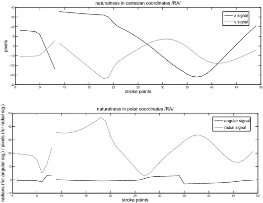
It is often the case that an appropriate representation of a problem leads to the optimal solutions. Expressing the naturalness in a polar coordinate system was tested to see if such a representation would reduce the complexity of the handwriting task. Fig. 4.6 plots the naturalness for an example character /ra/ in both the cartesian and the polar coordinate system. As we can see, the angular signal varies much less than the radial signal. Moreover, the long steady parts of the angular signal are followed by the parts where the angular signal change abruptly over short period of time. On the contrary, x and y signals in the Cartesian coordinate system vary about the same. This similar variance of x and y signal might result in easier modeling of the naturalness.

All of the presented trials in this dissertation were therefore carried out using the naturalness expressed in the cartesian coordinate system. Trials using the naturalness expressed in the polar coordinate system were carried out also and are discussed in Section 7.4.

4.6 Spacing Interval

The spacing interval of 8 pixels was found to produce the input/output signals that performed the best. This spacing interval was therefore mainly used thorough this study with all of the presented experiments being carried out with the 8 pixels data only. Several other spacing intervals were also tested, however these other values produced input signals, which varied over a timescale that was either too fast or too slow for standard RBF/sigmoid units. Comparison of the left and the right column in Fig. 4.5 and Fig. 4.7 shows that the signals made using the spacing interval of 4 pixels vary over a much slower timescale than the signals made using the spacing interval of 8

(44)

0 5 10 15 20 25 30 35 40 45 50

−10 0 10 20 30 40 50

naturalness in polar coordinates /RA/

stroke points

radians (for angular sig.) / pixels (for radial sig.)

angular signal radial signal

0 5 10 15 20 25 30 35 40 45 50

−40

−30

−20

−10 0 10 20 30 40

naturalness in cartesian coordinates /RA/

stroke points

pixels

x signal y signal

Figure 4.6: Naturalness in Cartesian and polar coordinates for character /RA/.

pixels. The curvature signals shown in Fig. 4.5 vary over different timescale with their values coming from an interval [−1,1], whereas the inertia signals shown in Fig. 4.7 not only vary over different timescale but also their values come from different intervals. The same hold true for their respective derivative estimates. The values for the inertia signals made using the spacing interval of 8 pixels come from an interval over [−10,10]. The spacing interval of 4 pixels produced the inertia signals, which come from an interval over [−5,5]. The difference in values causes no problem for modeling because all signals are normalized using the global factor a. It is the timescale that matters. The timescale for the curvature and the inertia signals made

(45)

using the spacing interval of 4 pixels was found to be too slow for standard RBF/sigmoid units. On the other hand, spacing intervals of more than 8 pixels produced the signals that vary too fast.

0 50 100 150 200 250

0

50

100

150

200

250

character /RA/ (8 pixels)

0 5 10 15 20 25 30 35 40 45 50

−10

−5 0 5 10

stroke points

inertia (8 pixels)

0 5 10 15 20 25 30 35 40 45 50

−10

−5 0 5

stroke points

inertia/dt (8 pixels)

0 50 100 150 200 250

0

50

100

150

200

250

character /RA/ (4 pixels)

0 10 20 30 40 50 60 70 80 90 100

−10

−5 0 5 10

stroke points

inertia (4 pixels)

0 10 20 30 40 50 60 70 80 90 100

−10

−5 0 5

stroke points

inertia/dt (4 pixels)

Figure 4.7: Inertia signals and their derivative estimates made using the spacing interval of 8 and 4 pixels.

(46)

Chapter 5 Analysis and Modeling of Naturalness in Handwritten Characters

5.1 Analysis of Naturalness

5.1.1 Canonical Correlation Analysis

The linear relationship between two sets of variables can be investigated using Canonical correlation analysis (CCA) [13, 14]. In the following, we interpret only the leading canonical variates, so by canonical correlation we always mean the first canonical correlation between the leading canonical variates.

Similarly, by canonical weights, we always refer to the weights corresponding to the leading canonical variates.

The second power of the canonical correlation explains shared variability between a pair of canonical variates but provides no information regarding how much variability in the original sets is explained by their respective canonical variates. This information can be obtained by computing the sum of squares of the loadings (correlations) between the canonical variates and their original variables, divided by the number of original variables in the

(47)

corresponding set. By multiplying the obtained number with the square of the canonical correlation, we finally obtain information concerning how much variability in the given set is explained by the variables in the other set. This information is referred to as the redundancy (for a given set). In equation form, the redundancy for a given set may be expressed as

redundancy= (

n

X

i=1

l²_i)/n∗r_c² (5.1) where n denotes the number of variables in a given set, l_i denotes the i-th loading and r_c the squared canonical correlation [30].

To begin with, we investigated the linear relationship between the naturalness and the input data extracted from the fontC strokes. 61 hiragana characters written by five people were examined; i.e. five people were each asked to write down all 61 hiragana characters. The input matrices are computed from the font, and are therefore identical for all writers. The naturalness matrices, however, are unique for each writer. The analysis was carried out for each writer as follows. For each j-th stroke of the i-th character (i= 1, ..,61), the input data matricesU_ij and the corresponding naturalness matrices V_ij were computed according to the data specification outlined in Chapter 4. The input and the naturalness matrices for strokes belonging to the same i-th character were respectively merged into a single input matrix U_i and naturalness matrix V_i. CCA was applied to all pairs U_i,V_i and the redundancy ofV_i was observed. Intuitively speaking, the redundancy of V_i represents the percentage of the variability in the naturalness V_i, which is explained by the variability of the corresponding input data Ui. Table 5.1 provides redundancies for all 61 examined characters of each respective writer. The very bottom row shows the average redundancy as calculated for each writer. It can be seen that the averages vary only slightly, with the

(48)

grand average being 0.3011. This means that for the five writers in our exper- iment, an average of 30.11% of the variability in the naturalness is explained by the variability in the input data.

Table 5.1: Redundancies for 61 examined hiragana characters.

character redundancy

wr1 wr2 wr3 wr4 wr5

B ”a” 0.3437 0.1521 0.3516 0.2051 0.1921 D ”i” 0.7870 0.5061 0.2401 0.1411 0.1964 F ”u” 0.4625 0.2090 0.4255 0.4442 0.5103 H ”e” 0.1508 0.4519 0.3621 0.4500 0.6337 J ”o” 0.3243 0.1865 0.3807 0.2675 0.1151 K ”ka” 0.1209 0.0410 0.2285 0.3106 0.4195 M ”ki” 0.4749 0.3980 0.3134 0.5378 0.3504 O ”ku” 0.6411 0.4812 0.7217 0.0540 0.5041 Q ”ke” 0.1934 0.0955 0.0933 0.1164 0.2770 S ”ko” 0.1497 0.3218 0.5304 0.4144 0.3159 U ”sa” 0.4821 0.4253 0.2812 0.6198 0.3366 W ”shi” 0.5981 0.5130 0.7304 0.8405 0.7619 Y ”su” 0.2357 0.1164 0.4770 0.2891 0.2345 [ ”se” 0.1764 0.2406 0.0568 0.3777 0.1665 ] ”so” 0.0405 0.0443 0.0264 0.3570 0.0540 _ ”ta” 0.2217 0.3186 0.3349 0.1376 0.0945 a ”chi” 0.0958 0.3561 0.2743 0.2054 0.4263 d ”tsu” 0.5212 0.6904 0.6152 0.4076 0.2757 f ”te” 0.5838 0.2343 0.5612 0.5999 0.5609 h ”to” 0.5456 0.8319 0.3667 0.3370 0.6780

”ra” 0.1072 0.0880 0.1989 0.1434 0.6296

”ri” 0.1102 0.1220 0.2016 0.0670 0.0252

”ru” 0.2431 0.0960 0.4580 0.1655 0.2368

”re” 0.1813 0.3736 0.1577 0.0753 0.1378

”ro” 0.3731 0.2596 0.3225 0.4491 0.2906

~ ”ma” 0.1496 0.3554 0.3552 0.3535 0.2939

”mi” 0.3449 0.2945 0.2874 0.3243 0.2833 continued . . .