Instructions for use
T itle A comparison principle for singular diffusion equations with spatially inhomogeneous driving force for graphs
A uthor(s ) Giga,M.-H.; Giga,Y .; R ybka,P.
C itation Hokkaido University Preprint S eries in Mathematics, 981: 1-43
Is s ue D ate 2011-8-5
D O I 10.14943/84128
D oc UR L http://hdl.handle.net/2115/69788
T ype bulletin (article)
A comparison principle for singular diffusion
equations with spatially inhomogeneous
driving force for graphs
M.-H. Giga, Y. Giga and P. Rybka
1
Introduction
As a continuation of [GG98Ar], [GG01Ar] this paper studies a degenerate nonlinear parabolic equation (in one space dimension) whose diffusion effect is very strong at particular slopes of unknown functions. We are in par-ticular interested in an equation, where the driving force term is spatially inhomogeneous. A typical example is a quasilinear equation
ut=a(ux)[W′(ux)x+σ(t, x)], (1.1)
where W is a given convex function on R but may not be of class C1 so
that its derivative W′ may have jump discontinuities; herea is a given
non-negative continuous function andσ is a given smooth function depending on
x and also ont, whereut and ux denote the time and the space derivative of
u=u(t, x).
As explained in detail in [GG98Ar] the equation is viewed as an evolution law of the graph of u moved by an anisotropic mean curvature flow V =
M(n) (κγ +σ) with a singular interfacial energy density γ, where κγ is a
weighted curvature and M is mobility; V denotes the normal velocity of the evolving curve in the direction of n. (The quantity κγ formally equals
(γ′′+γ)κwith curvatureκandγ =γ(θ) is an interfacial density as a function
of the argument θ of n= (cosθ,sinθ).)
Our eventual goal is to establish a kind of the theory of viscosity solutions for a class of equations including (1.1) as a particular example so that we are able to construct a global-in-time solution for example for periodic initial data. In this paper we give a new notion of viscosity solutions for (1.1) and establish a comparison principle.
Ifσ in (1.1) is independent ofx, the theory of viscosity solutions has been already established in [GG98Ar], [GG01Ar]. Even in this simpler case the quality (W′(u
x))x turns to be nonlocal so conventional viscosity theory does
not work. For example if W(p) =|p|, thenW′′(p) is twice the delta function
so that (1.1) becomes
ut=a(ux)[2δ(ux)uxx+σ(t)] (1.2)
break. Here L is the length of a facet (which is a nonlocal quantity) and
χ=±1,0 is a transition number of the facet depending upon local behavior ofunear facet. For example, ifuis ‘concave’ near the facet, thenχshould be
−1. When σ is spatially homogeneous, this hypothesis that a facet does not break is justified either by viscosity theory developed by [GG98Ar], [GG99] or by subdifferential theory [FG] (in the case σ ≡0), in the sense that such a solution is an appropriate limit of solutions to strictly parabolic problems. When W is piecewise linear andσ is independent ofx, then (1.1) is analyzed in [T], [AG1] for a very restrictive class of piecewise linear unknown functions whose slopes belong to jump discontinuities ofW. Their ’admissible’ solution is actually a solution in viscosity sense [GG98Ar].
Ifσ depends on the space variable, the hypothesis that all facets do not break is no longer true. For example, if we postulate this hypothesis, then the speedutof a facet with slope zero ofuof (1.2) equalsa(0)[2χ/L+−
R σdx], where R− denotes the average over the facet. As noticed in [GG98Pit] if we
assigned the speed in this way the solution may not enjoy in general the comparison principle. This shows that such a ’solution’ is not obtained as a limit of approximate problems satisfying the comparison principle. On the other hand if |σx| is sufficiently small compared with the length of facets,
such a solution is known to enjoy comparison principle [BGN].
If a is a constant, say a ≡ 1, and σ is independent of t, (1.1) can be viewed as a subdifferential formulation
ut∈ −∂ϕ(u), (1.3)
where ϕ is an energy which formally equals
ϕ(u) =
Z T
[W(ux)−σ(x)u]dx;
for simplicity we assumed here a periodic boundary condition so that T =
R/ωZ. As observed in [GG98DS] for (1.3) a general theory of subdifferential equations in a Hilbert space L2(T) provides not only unique existence of the
solution but also the value of right derivativedu+/dt(ofuas a function with
value in H). A general theory further yields
d+u/dt=−∂0ϕ(u),
In [GG98DS] it is observed that∂0ϕcan be calculated by solving an obstacle
problem. Let us review their observation. Since the condition
f ∈ −∂ϕ(u)
is equivalent to
f(x) = ηx(x) +σ(x), η(x)∈∂W(ux(x)), a.e. x∈T,
the quantity
−∂0ϕ(u) =
(
(W′(u
x(x)))x+σ(x) if ux ∈/ P
η0
x(x) +σ(x) if ux ∈P ,
(1.4)
where P is the jump discontinuity ofW′ and uis assumed to be of class C2
and P-faceted [GG98Ar]. Here, η0 minimizes
{
Z
F
|ηx+σ|2dx ; η ∈∂W(ux(x))} (1.5)
under suitable boundary condition at the end of the facet F depending on whether u is ‘convex’ or ‘concave’ near F. This is a convex minimizing problem so a unique minimizer always exists. Moreover, if σ is independent of x, ηx must be constant and ηx0+σ=χ/L+σ. If σ depends on x,ηx0+σ
may not be a constant over F and this is one reason why the speed may not be a constant on F when σ depends on x. The subdifferential equation (1.3) can be approximated by a smooth parabolic problem, so the solution is expected to enjoy the comparison principle. Thus, it is natural to guess that
η0
x+σ gives a candidate for the value of
ΛσW(u)(x)) = (W′(ux))x+σ(x) (1.6)
when W′ has jump discontinuities. Note that this quantity agrees with the
minimal velocity profile proposed by [Rs] as observed in [GG98DS].
Unfortunately, a general equation (1.1) cannot be viewed as a subdiffer-ential equation (1.3). However, we still use the value (1.4) to define (1.6). We establish a notion of viscosity solutions by assigning the value Λσ
W by
breaks. The idea of the proof of the comparison principle is similar to that of [GG98Ar] except for a simplification of handling end points of facets ob-served by [GG01Ar] and the use of continuity of Λσ
W(u) under translation of
a faceted region which is obvious when σis constant. So we have to study an obstacle problem in this paper carefully. Let Λ(F)(x) be a quantity defined by
Λ(F)(x) =η0
x(x) +σ(x) , x∈F,
where η0 is the minimizer of (1.5). In particular, we prove that
Λ(Fµ) (x−µ)→Λ(F) (x)
as µ→0, where Fµ=F −µ={x|x+µ∈F}provided that σ
x is bounded.
Moreover, the convergence is uniform with respect to F provided that F
is bounded. This problem can be viewed as a stability problem for (1.5) with respect to perturbations of σ. Since our obstacle problem is convex, it is not difficult to prove these facts. We also need comparison results (maximum principle) for Λσ
W so see that it behaves like curvature or usual
second derivatives. It is often convenient to consider ξ = η +Rx
σ as a variable, instead of η itself, so we shall use variable ξ. We warn the reader that in Section 5 we will use differently defined ξ.
To establish the comparison principle we argue by contradiction using the doubling variables technique. Letube a subsolution andvbe a supersolution. We are interested in maximizers of
u(t, x)−v(s, y)−Bε(x−y)−(t−s)2/δ−γ/(T −t)−γ/(T −s)
for small ε, δ, γ > 0. Here Bε = ²B(x/ε) , B(x) ∽ x2 for large x and B
is a (non-negative) faceted C2 convex function with B(0) = 0. This choice
of a test function B is different from [GG98Ar] and this choice simplifies the argument. We use sup-convolutions with a faceted function to regularize the problem as in [GG98Ar]. The quantity Λσ
W behaves like usual second
derivative in the sense that it satisfies the maximum principle. At the final stage we have to compare Λ(Fµ) and Λ(F) which is trivial whenσis constant,
because it is independent of µ.
is expected [GG99] but we do not intend to include any progress in this direction in the present paper. A general existence result through Perron’s method is almost the same as that in [GG98Ar], though we do not state it explicitly. Instead, we give a couple of examples of solutions.
Recently, besides examples in [GG98DS] several semi-explicit variational solutions are constructed for (1.1) for a special choice of M, σ and γ by solving a free boundary problem [GR1], [GR2], [GGR]. Their variational solutions are expected to be our viscosity solutions. In this paper we shall confirm this consistency at least for some typical examples.
We do not know much about surface evolutions. In surface evolving problems a facet may not stay as a facet even if σ ≡ 0 see e.g. [BNP], [BNP1], [BNP2] and [BNP3]. A notion of a generalized solution is established and a comparison principle is proved in [BN], see also [BGN]. However, the existence of solution is known only when initial surface is convex see [BCCN]; note that their problem is formulated for V = γκγ where mobility parallels
the interfacial energy.
The bibliographies of review papers [GGK], [G04], [GG04], [GG10] in-clude several articles dealing with anisotropic curvature flow equations with singular interfacial energy or singular diffusion equations. Here we only men-tion a few recent works related to this topic but not included there. In partic-ular, we have in mind the approach developed by Mucha and Rybka, which is based on an original definition of composition of multivalued operators, see [MR1], [MR2]. So far it is restricted to one dimension by allows to study facet evolution for quite general data and regularity of solutions.
2
Variational properties of nonlocal curvature
with a nonuniform driving force term
We shall give a variational characterization of the quantity Λσ
W, which is
formally defined by
Λσ
W(u) (x) = (W′(ux))x+σ(x), (2.1)
by solving an obstacle problem. This characterization enables us to derive various important properties to establish the theory of viscosity solutions for singular diffusion equations.
2.1
An obstacle problem
Let Z be a real-valued C2 (or C1,1) function defined in a bounded interval
I, where I = (a, b). For a given ∆>0 let KZ
χlχr be the set of all ξ ∈H
1(I)
satisfying
Z(x)−∆/2≤ξ(x)≤Z(x) + ∆/2 forx∈I (obstacle condition) (2.2) and
ξ(a) =Z(a)−χl∆/2, ξ(b) =Z(b) +χr∆/2 (boundary condition). (2.3)
Here, χl and χr take values ±1. LetJχZlχr be the functional onL
2(I) defined
by
JχZlχr(ξ) =
(Rb a |ξ
′(x)|2 dx, ξ ∈KZ χlχr
∞, otherwise.
In this subsection, we suppress the dependence with respect toZ since we fix
Z. By the definition ofJχlχr, it is easy to see that infJχlχr is theH
1 distance
from zero to convex closed set Kχlχr in H
1. Thus, J
χlχr admits a unique absolute minimizer denoted by ξχlχr. Evidently, ξχlχr ∈ H
1(I) ⊂ C1/2(I)
by the Sobolev embedding. In fact, it is C1,1 as proved in [[KS], Chap II
Theorem 7.1]. (In [KS] the regularity of multidimensional obstacle problem is also discussed.) In our one-dimensional case it is easy to prove that ξχlχr is C1,1 since the obstacle is C1,1 as described below.
Forξ ∈ H1(I) let D
We say thatD+is theupper coincidenceset whileD−is thelower coincidence
set.
Definition 2.1. We say thatξ∈Kχlχr satisfies theconcave-convex condition if ξ is concave outside the upper coincidence set D+ and convex outside the
lower coincidence set D−, i.e.,ξ′′ ≤0 outsideD+ and ξ′′≥0 outside D−. In
particular, ξ isC1,1 inI and ξ′′ = 0 outsideD
− ∪ D+.
Proposition 2.2 (A characterization of the minimizer). The function
ξ ∈Kχlχr is the minimizer of Jχlχr if and only ifξ fulfills the concave-convex
condition. In particular, ξχlχr isC
1,1 inI and
sup
x∈I
|ξχ′′lχr(x)| ≤sup
x∈I
|Z′′(x)|. (2.4)
Proof. By convexity of Jχlχr and the uniqueness of the minimizer, ξ∈Kχlχr is the absolute minimizer if and only if ξ is a local minimizer ofJχlχr i.e.,
Z
Dc
+
ξ′ϕ′dx≥0, Z
Dc
−
ξ′ϕ′dx≤0
for all ϕ ∈ H1(I) satisfying ϕ(a) =ϕ(b) = 0 and ϕ ≥ 0 inDc
+ =I\D+ and
for allϕ ∈H1(I) satisfyingϕ(a) =ϕ(b) = 0 andϕ≥0 inDc
− =I\D− by the
obstacle condition (2.2) and the boundary condition (2.3). This is equivalent to the concave-convex condition; for equivalence of convexity in distribution sense and strong convexity see e.g., Schwartz [S] or H¨ormander [H]. The remaining statement is a simple consequence of the concave-convexity con-dition. ¤
As a trivial application we give two cases, where the minimizer is explicitly written.
Corollary 2.3.
(i) If the concave hull Zcave of Z inI is smaller than Z + ∆, i.e., Zcave ≤
Z+ ∆ inI, then ξ+−=Zcave−∆/2.
(ii) If the straight line functionξ(x) =ξ(a)+(Z(b)−Z(a)+∆) (x−a)/(b−a)
fulfills the obstacle condition (2.2), it is the minimizer ofJ++ provided
that ξ(a) = Z(a)−∆/2 and ξ(b) = Z(b) + ∆/2. Here, J++ = Jχlχr
2.2
Comparison principle
So far we have fixed the interval I to defineξχlχr. We shall study the depen-dence of ξ′
χlχr upon I. To clarify this we write Jχlχr, I instead of J
Z
χlχr and
ξχlχr, I instead ofξ
Z
χlχr. We set
ΛZχl′χr(x, I) =
dξχlχr, I(x)
dx . (2.5)
It is easy to observe that this quantity agrees with η0
x+σ, when Z equals
a primitive of σ. It is sufficient to take ξ = η+Z. The reason we write Z′
instead of Z is that the derivative of ξZ
χlχr depends on Z only through its derivative. We suppress Z′ in (2.5) when we fix Z. We shall write Λ
−+ etc.
instead of writing Λ{−1},{+1}.
Theorem 2.4 (Comparison principle). Assume thatI1andI2are bounded
open intervals.
(i) IfI2 ⊂I1, then
Λ−−(x, I2)≤Λ±±(x, I1)≤Λ++(x, I2) for x∈I2. (2.6)
(ii) Ifa≤c < b≤d for I1 = (a, b), I2 = (c, d), then forx∈(c, b)
Λ±−(x, I1)≤Λ+±(x, I2), Λ−±(x, I2)≤Λ±+(x, I1). (2.7)
This can be proved by a comparison principle for parabolic equations by an approximation as is done in Giga-Gurtin-Matias [GGM]. However, since the problem is one dimensional, we rather give an elementary proof.
Proof. It suffices to prove
(a) Λ++(x, I1)≤Λ++(x, I2), Λ−−(x, I2)≤Λ−−(x, I1) for x∈I2 ⊂I1,
(b) Λ−+(x, I1)≤Λ++(x, I1), Λ−−(x, I1)≤Λ−+(x, I1) and
Λ+−(x, I1)≤Λ++(x, I1), Λ−−(x, I1)≤Λ+−(x, I1) for x∈I1.
with I1 = (a, c), I2 = (a, b) for c (≥b) sufficiently close to b. We divide the
situation into two cases depending on the structure of the coincidence set of the minimizer ξ2 =ξ++,I2.
Case 1. There is δ > 0 such that (b −δ, b) is not included in any
coincidence set and the point b−δ is a point of lower coincidence set.
In this situation the graph ofξ2 is a straight line on (b−δ, b) and ξ2(b) =
Z(b) + ∆/2. We extend ξ2(x) for x≥b such that the slope of ξ2 is constant
for x ≥b−δ. The extension is still denoted ξ2. If Z(c) + ∆/2≥ξ2(c), it is
clear that ξ1 = ξ2 on I2, where ξ1 = ξ++,I1. If Z(c) + ∆/2 < ξ2(c) and c is
close to b, the graph of ξ1 is a straight line from (b−δ′, c), 0 < δ′ < δ and
ξ1(b−δ′) = Z(b−δ′)−∆/2 with ξ1′(b−δ′) =Z′(b−δ′). Moreover, ξ1 (≤ξ2)
agrees with the concave hull of Z(x)−∆/2 in (b−δ, b−δ′). Thus, it is clear
that ξ′
1 ≤ξ2′ forx∈(b−δ, b) where ξi′ =dξi/dx.
Case 2. The minimizer ξ2 agrees with the convex hull of Z(x) + ∆/2 in
(b−δ, b) for some (small) δ >0.
Ifcis sufficiently close tob, thenξ1 agrees with the convex hull ofZ(x) +
∆/2 in (b−δ, c). By comparison of slopes of the convex hull it is clear that
ξ′
1 ≤ξ′2 on (b−δ, c). This completes the proof of (a).
We next prove (b). By symmetry it suffices to prove one of four inequal-ities. We shall prove that Λ−−(x, I1)≤Λ−+(x, I1).
Letξ =ξ−−,I1 be the minimizer such thatξ′ = Λ−−(x, I1) andη(= ξ−+,I2)
be the minimizer such that η′ = Λ
−+(x, I2). By the structure of minimizer
(Proposition 2.2) if ξ(x0) = η(x0) for a < x0 < b, then ξ = η on (a, x0).
Thus there exists the maximum x∗ ≥ a such that ξ = η on (a, x∗). If
ξ(x∗) =η(x∗) = Z(x∗) + ∆/2, thenη is a convex hull ofZ(x) + ∆/2 in (x∗, b)
whileξis a concave hull of max (Z(x)−∆/2, ξ(x∗)I(x)) whereI(x) =−∞for
x6=x∗ and I(x∗) = 1. Thus it is easy to see that ξ′ ≤η′ onI1. A symmetric
argument in the case of ξ(x∗) = η(x∗) = Z(x∗)−∆/2 yields ξ′ ≤ η′ on I1.
We have thus proved that Λ−−≤Λ−+.
2.3
Stability of curvature like quantity
essentially known in the literature e.g. [Rd, p.156, Chapter 5, Theorem 4.5 and Remark 4.6]. However, we rather give a proof for the reader’s convenience since the situation is slightly different.
We recall several stability properties ofJχlχr. Let{Z
k}∞
k=1 be a sequence
of real-valued C2 (or C1,1) functions inI, whereI = (a, b). In this subsection
we fix χlχr, so we often suppress its dependence and simply write JχZlχr for
J and JZk
χlχr instead of J
k.
Proposition 2.5 (Lower semicontinuity). Assume that Zk uniformly
converges to Z as k → ∞, i.e., Zk → Z in C(I). Assume that ξ
k weakly
converges to ξ inL2(I) as k→ ∞. Then J(ξ)≤lim inf
k→∞Jk(ξk). Proof. We may assume that ξk ∈ KZ
k
. Since ξk−Zk converges to ξ−Z
weakly in L2(I) and sign is conserved through weak limit, we observe that
ξ ∈ KZ. The desired conclusion now follows from the lower semicontinuity
of H1-norm with respect to L2-weak convergence. ¤
Proposition 2.6 (Approximability). Assume that Zk converges to Z,
with its first derivative, uniformly in I as k → ∞, i.e., Zk → Z in C1(I).
Then for each ξ ∈ L2(I) there is a sequence ξ
k → ξ in L2(I) such that
J(ξ) = limk→∞Jk(ξk).
Proof. We may assume that ξ ∈KZ since otherwise ξ /∈KZk
for sufficiently large k. We setξk =ξ−Z+Zk and observe that ξk is in KZ
k
by (2.3) and (2.4). Since Zk →Z, (Zk)′ →Z′ uniformly in I as k→ ∞, the convergence
J(ξk)→J(ξ) and ξk→ξ (ask → ∞) in L2(I) is easily verified. ¤
These two above Propositions say that Jk converges to J in the sense of
Mosco, i.e., both strong and weak Γ− limits of Jk equal J. Thus we easily
obtain the convergence of minimizers.
Proposition 2.7 (Convergence of minimizers). Assume that Zk → Z
inC1(I)ask → ∞. Letξk
χlχr be the minimizer ofJ
k
χlχr. Thenξ
k
χlχr converges
to ξχlχr in L
2(I) which is the minimizer of J
χlχr.
Proof. Applying Proposition 2.6 to ξχlχr, we observe that {minJ
k}∞ k=1 is
bounded. Since H1(I) is compactly embedded in L2(I), ξk
χlχr subsequently converges to an elementζ ∈L2(I) ask → ∞. By Proposition 2.5, we observe
that
J(ζ)≤lim inf
k→∞ min J
k.
ξk →ξ inL2(I) such that Jk(ξk)→J(ξ) as k→ ∞. Thus
J(ζ)≥lim inf
k→∞ min J
k.
Therefore, J(ζ)≤ J(ξ) soζ must be the unique minimizer of J. Thus ξk χlχr converges ξχlχr without taking a subsequence. ¤
We define Λk
χlχr(x, I) by (2.5) where Z is replaced by Z
k. We simply
write Λk
χlχr in place of Λ
k
χlχr(x, I) and Λχlχr instead of Λ
Z′
χlχr(x, I) in the next Theorem.
Theorem 2.8 (Continuity with respect to Z′). Assume that
sup
k≥1
sup
x∈I
|(d/dx)2Zk(x)|<∞ and (Zk)′ →Z′ in C(I).
Then Λk
χlχr →Λχlχr in C(I)as k → ∞.
Proof. We may assume that Zk →Z in C1(I) by adding a constant to fix a
value at some point of I, for example Zk((a+b)/2) = 0, Z((a+b)/2) = 0.
By Proposition 2.7 we observe that ξk
χlχr → ξχlχr in L
2(I). By Proposition
2.2 our assumption on the bound of the second derivative of Zk implies
that |(d/dx)2ξk
χlχr| is bounded by (2.4). Thus ξ
k
χlχr → ξχlχr in C
1(I) so
Λk
χlχr →Λχlχr inC(I). ¤
We are now in position to state continuity of Λχlχr with respect to I. This notion will be explained below.
Theorem 2.9.
(i) Let Z be a C2 (or locally C1,1) function on R. Then ΛZ′
χlχr(x, I) is
continuous with respect to I.
(ii) Assume furthermore that|Z′′(x)|is bounded inR. Then for eachr >0
lim
µ→0 0<bsup−a<r a<x<bsup |Λ
Z′
χlχr(x,(a, b))−Λ
Z′
χlχr(x−µ,(a−µ, b−µ))|= 0.
(The convergence is uniform in Z′ for Z such that |Z′′| ≤ M
0 for a given
constant M0 >0.)
We have to clarify the continuity with respect to I. For two bounded intervals I = (a, b) and J = (c, d) there is a unique affine map A: x 7→y =
ak, bk of Ik = (ak, bk) tend to a and b, respectively. Let F be a mapping:
I7→F(I)∈C(I). We say thatF is continuous with respect toI if F(Ik)◦Ak
converges to F(I) in C(I), as k→ ∞ for any Ik →I, where Ak is the affine
map which maps I toIk.
Proof. These assertions easily follow from Theorem 2.8, once we compare ΛZ′
χlχr(x, I) with Λ
Z′
χlχr(A
k(x), I
k), both defined on I, here Ak is the affine
transformation mapping I to Ik, when Ik → I. (In the assertion (ii) this
affine map is just a translation.) ¤
2.4
Nonlocal curvature with a nonuniform driving force
term
In order to define the nonlocal curvature Λσ
W(u) formally given by (2.1) we
recall basic assumptions on W as in [GG98Ar] and a class of function u so that Λσ
W(u) is well-defined.
(W) Let W be a convex function on R with values in R. Assume that W is of class C2 outside a closed discrete set P and that W′′ is
bounded in any compact set except all points inP.
We shall always assume (W) in this paper. By definition the set P is either a finite set or a countable set having no accumulation points in R. If
P is nonempty, P is of form {pj}jm=1, {pj}∞j=−∞, {rj}−j=1−∞ or {pj}∞j=1 with
limj→∞ pj =∞,limj→−∞ rj =−∞, where the pj’s and rj’s are arranged in
strictly increasing sequencespj < pj+1, rj < rj+1and mis a positive integer.
We recall a notion of a faceted function. Let Ω be an open interval. A function f in C(Ω) is called facetedat x0 with slope p on Ω (or p-faceted at
x0) if there is a closed nontrivial finite interval I(⊂ Ω) containing x0 such
that f agrees with an affine function
ℓp(x) = p(x−x0) +f(x0) in I
and f(x) 6= ℓp(x) for all x ∈ J\I with some neighborhood J(⊂ Ω) of I.
The interval I is called afaceted region of f containingx0 and is denoted by
R(f, x0). A function f is called P-faceted at x0 if it is p-faceted at x0 for
We introduce theleft transition numberχl =χl(f, x0) and theright
tran-sition number χr =χr(f, x0) by
χl=
(
+1 if f ≥ℓpi in {x∈J|x≤x0}
−1 if f ≤ℓpi in {x∈J|x≤x0}
χr=
(
+1 if f ≥ℓpi in {x∈J|x≥x0}
−1 if f ≤ℓpi in {x∈J|x≤x0}
if f is pi-faceted at x0. The quantityχ= (χl+χr)/2 is called thetransition number describing the sign of Λσ
W when σ ≡0.
Definition 2.10. We assume that σ is a real-valued Lipschitz function on
an open interval Ω and Z is its primitive, moreover, (W) holds. We assume thatf ∈C(Ω)pi-faceted atx0 ∈Ω withpi ∈P. Then we define thenonlocal curvature Λσ
W by
ΛσW(f) (x0) = ΛZ
′
χlχr(x, I); the right hand side is defined by (2.5) with ∆ = W′(p
i + 0)−W′(pi −0)
and I is the faceted region R(f, x0). If f is twice differentiable at x0 and
f′(x
0)∈/ P, we set, as expected,
ΛσW(f) (x0) =W′′(f′(x0))f′′(x0) +σ(x0).
Remark 2.11. If σ is a constant, so that Z is an affine function, the
min-imizer ξχlχr of J
Z
χlχr is always a straight line function (cf. Corollary 2.3 for the case χ= 1 or−1). Thus, it is easy to observe that
ΛσW(f) (x0) =χ∆/L(f, x0) +σ(x0)
when f is pi-faceted at x0, where L(f, x0) is the length of the faceted region
R(f, x0). In particular, our new quantity agrees with the weighted curvature
ΛW(f, x0), defined in [GG98Ar] when σ ≡ 0. Like ΛW(f, x0), the quantity
Λσ
W depends on W only through its second distributional derivative.
We conclude this section by rewriting Comparison Principle and Conti-nuity with respect to translation in terms of ΛσW. Let CP2(Ω) be the set of
f ∈ C2(Ω) such that f is P-faceted at x
0 whenever f′(x0) ∈ P. For such
a class of function the nonlocal curvature Λσ
W(f) (x) is well-defined for all
Theorem 2.12 (Comparison). Assume(W)and thatσ is locally Lipschitz and in addition f, g ∈ C2
P(Ω) and x0 ∈ Ω. If maxΩ(f −g) = (f −g) (x0),
then Λσ
W(f) (x0)≤ΛσW(g) (x0).
Theorem 2.13 (Continuity). Let us suppose that the hypotheses of
The-orem 2.12 concerning W and σ. We assume that f ∈ C(Ω) is pi-faceted
at x0 −η and g be pi-faceted at x0 − η and pi ∈ P. Assume moreover,
R(f, x0)−η=R(g, x0−η). Then
ΛσW(g) (x0−η)→ΛσW(f) (x0) as |η| →0.
3
Definitions of generalized solutions
The goal of this section is to define a generalized solutions (in the viscosity sense) for evolution equations of the form
ut+F(t, ux,ΛσW(u)) = 0 (3.1)
when W is a singular interfacial energy. Such a notion is given when σ ≡0 in [GG98Ar]. Our definition will be a natural extension to the case when
σ 6≡ 0. In this section, we shall also give several equivalent definitions for later use.
3.1
Admissible functions and definition
We first recall a natural class of test function. Let us set Q = (0, T)×Ω, where Ω is an open interval andT > 0. LetAP(Q) be the set of alladmissible
functions ψ onQ in the sense of [GG98Ar] i.e., ψ is of the form
ψ(x, t) =f(x) +g(t), f ∈CP2(Ω), g ∈C1(0, T).
For our equation we often assume that
(F1) F is continuous in [0, T]×R×R with values in R,
(FL) (Lipschitz continuity.) There is a constant C =CF,T such that
|F(t, p, X)−F(t, p, Y)| ≤C(1+|p|)|X−Y|for allt∈[0, T], p, X, Y ∈R.
(FT) (Uniform continuity in curvature and time.) For each K the function
F(t, p, X) is uniformly continuous in [0, T]×[−K, K]×R.
The third assumption in rather standard when W ≡0 and σ is Lipschitz so that ΛσW(u) =σ. A typical example of (3.1) satisfying (F1), (F2), (FL) and (FT) is of the form
ut−a(ux) ΛσW(u)−C(t) = 0 (3.2)
where
F(t, p, X) =−a(t, p)X;
here a ∈C(R) satisfies 0 ≤a(p) ≤C(|p|+ 1) for all p ∈R, C ∈C[0, T]. If
a(p) = (1 +p2)1/2 and C ≡0, then (3.2) says that the normal velocity V of
the graph of u equals the nonlocal curvatures i.e., V = Λσ
W. The condition
(FT) is redundant if F is independent of t since (FL) implies (FT).
The driving force term σ may depend on t. Here is an assumption we often use.
(S) The function σ ∈ C¡
[0, T]×Ω¢
is Lipschitz in space uniformly in time, i.e. there is a constant LT such that
|σ(t, x)−σ(t, y)| ≤LT|x−y|
for all t ∈[0, T], x, y ∈Ω.
We are now in position to give a notion of a generalized solution in the viscosity sense.
Definition 3.1. Assume (W), (S), (F1), (F2). A real-valued function u
on Q is a (viscosity) subsolution of (3.1) in Q if the upper-semicontinuous envelope u∗ <∞ in [0, T)×Ω and
ψt(ˆt,xˆ) +F
³
ˆ
t, ψx(ˆt,xˆ), ΛWσ(ˆt,·)(ψ(ˆt)) (ˆx)
´
≤0 (3.3)
whenever ¡
ψ,(ˆt,xˆ)¢
∈AP(Q)×Qfulfills
max
Q (u
Here ψ(ˆt) is a function on Ω defined byψ(ˆt) =ψ(ˆt,·) and u∗ is defined by
u∗(t, x) = lim
ε↓0 sup{u(s, y)| |s−t|< ε, |x−y|< ε, (s, y)∈Q}
for (t, x) ∈ Q and u∗ = (−u∗). A (viscosity) supersolution is defined by
replacing u∗(< ∞) by the lower-semicontinuous envelope u
∗(> −∞), max
by min in (3.4) and the inequality (3.3) by the opposite one. If u is both a sub- and supersolution, u is called a viscosity solution or a generalized solution. Hereafter we avoid using the word viscosity. Function ψ satisfying (3.4) is called a test function of u at (ˆt,xˆ). The monotonicity (F2) and the convexity (W) say that the equation is at least degenerate parabolic, so by comparison (Theorem 2.12) it is easy to see thatψ ∈AP(Q) is a subsolution
in Q if (and only if)ψ satisfies
ψt(t, x) +F
³
t, ψx(t, x), ΛWσ(t,·)(ψ(t))(x)
´
≤0
for all (t, x)∈Q.
3.2
An equivalent definition
To show comparison principle for sub- and supersolutions, it is convenient to recall equivalent definitions. One of them is regarded as an infinitesimal version. Such a definition is given in [GG98Ar] when σ ≡0. It is simplified by [GG01Ar]. We give a definition which is a natural extension of the one in [[GG01Ar], Theorem 4.3].
We first recall upper time derivations on a faceted region. Let ϕ be a function on Q and (ˆt,xˆ) ∈ Q. Assume that ϕ(ˆt,·) ∈ C(Ω) is p-faceted at
x∈Ω with p∈P. We define
T+
P ϕ(ˆt,xˆ) = {τ ∈R | there are a modulus
ω and three positive numbers δ, δ+, δ− such that
ϕ(t, x)−ϕ(ˆt,xˆ)≤τ(t−ˆt) +p(x−xˆ) +ω(|ˆt−t|)|t−tˆ|
for (t, x)∈(ˆt−δ, ˆt+δ)×N˜−1(ϕ(ˆt,·),ˆt;δ
+, δ−)},
where ˜N−1 denotes a semineighborhood ofR(ϕ(ˆt,·),xˆ) defined in [GG98Ar];
˜
N−1. Let f ∈C(Ω) be p-faceted at x
0 ∈Ω withp∈P. We set
Nχr(f, x0;δ+) =
(
{x∈Ω|supR(f, x0)< x≤supR(f, x0) +δ+} if χr(f, x0) = −1,
∅ if χr(f, x0) = 1
Nχl(f, x0;δ−) =
(
{x∈Ω|infR(f, x0)−δ− ≤x <infR(f, x0)} if χl(f, x0) = −1,
∅ if χl(f, x0) = 1
and the set ˜N−1 is defined by
˜
N−1(f, x0;δ−, δ+) = R(f, x0)∪Nχr(f, x0;δ+)∪Nχl(f, x0;δ−). The set ˜N+1 is defined by
˜
N+1(f, x0;δ−, δ+) = ˜N−1(−f, x0;δ−, δ+).
An element of TP+ϕ(ˆt,xˆ) is an upper time derivative at (ˆt,xˆ). The set of lower time derivative defined by
T−
P ϕ(ˆt,xˆ) = −T−+P(−ϕ) (ˆt,xˆ).
We next recall a class of functions (not necessarily admissible) for which upper time derivative is well-defined on a faceted region. The following defi-nition is an improved one in [GG01Ar] not the original one in [GG98Ar]. In [GG01Ar] Q may not be noncylindrical but here we consider a simple case
Q= (0, T)×Ω.
Definition 3.2. Let ϕ : Ω →R be an upper-semicontinuous function. For
(ˆt,xˆ) ∈ Q assume that ϕ(t,·) ∈ C(Ω) for t near ˆt. We say that ϕ is an (infinitesimally) admissible superfunction at (ˆt,xˆ) in Q if one of following three conditions holds.
(A) The function ϕ(ˆt,·) is P-faceted (in Ω) at ˆx ∈ int R(ϕ(ˆt,·),xˆ). The set TP+ϕ(ˆt,xˆ) is nonempty.
(B) There is (τ, p, X)∈ P+ϕ(ˆt,xˆ) with p /∈P, where P+ denotes the set of
parabolic semijets in Q [CIL], [GG98Ar].
We say that ϕ is an admissible subfunction at (ˆt,xˆ) in Q if ϕ is an ad-missible superfunction with P replaced by −P. We implicitly assume that
R¡
ϕ(ˆt,·),xˆ¢
does not touch the boundary of Ω. We are now in position to give a definition of subsolution in the infinitesimal sense.
Definition 3.3. Assume (W), (S), (F1), (F2). A real-valued function u on
Q is a subsolution in the infinitesimal sense of (3.1) (in Q) if u∗ < ∞ in
[0, T)×Ω and the following conditions are fulfilled. For (ˆt,xˆ) let ϕ be an admissible superfunction at (ˆt,xˆ) in Q such that ϕ is a test function of uat (ˆt,xˆ), i.e., (3.4) holds. Then
(i) τ +F³ˆt, ϕx(ˆt,xˆ),ΛσW(ˆt,·)(ϕ(ˆt,·))(ˆx)
´
≤0 for all τ ∈ TP+ϕ(ˆt,xˆ) if (A) in Definition 3.2 holds;
(ii) τ+F(ˆt, p, W′′(p)X+σ(ˆt,xˆ))≤0 for all (τ, p, X)∈ P+ϕ(ˆt,xˆ) if (B) in
Definition 3.2 holds;
(iii) τ +F(ˆt, p, σ(ˆt,xˆ)) ≤ 0 for all (τ, p,0)∈ P+ϕ(ˆt,xˆ) if (C) in Definition
3.2 holds and
(u∗−ϕ) (ˆt, x)<max
Q (u ∗ −ϕ)
for all x∈R¡
ϕ(ˆt,·),xˆ¢
\{xˆ} near ˆx.
The definition of supersolution in the infinitesimal sense is given by re-placing u∗(< ∞) by u
∗(> −∞), max by min in (3.4), supersolution by
subfunction, TP+ by TP−,P+ by P− and the inequalities in (i), (ii), (iii) by
the opposite ones. It turns out that Definition 3.1 and Definition 3.3 are equivalent.
Theorem 3.4 (Equivalence). Assume (W), (S), (F1), (F2). A real-valued
functionuonQis a subsolution (resp. supersolution) of (3.1) inQif and only if u is a subsolution (resp. supersolution) of (3.1) in Q in the infinitesimal sense.
course we need trivial modifications for example ΛW
¡
ψ(ˆt,·),xˆ¢
< 0 should be replaced by χ¡
ψ(ˆt,·),xˆ¢ <0.
Lemma 3.5 (Zero curvature). Let u be a subsolution of (3.1) in Q.
Assume that ϕ ∈AP(Q) and that
max
Q (u
∗−ϕ) = (u∗−ϕ) (ˆt,xˆ)
for (ˆt,xˆ) ∈ Q. If ˆx is an end point of a faceted region R¡
ϕ(ˆt,·),xˆ¢
with
ϕx(ˆt,xˆ)∈P and (u∗−ϕ) (ˆt, x)<(u∗−ϕ) (ˆt,xˆ) for all x∈R
¡
ϕ(ˆt,·),xˆ¢
near ˆ
x, then
ϕt(ˆt,xˆ) +F
¡ˆ
t, ϕx(ˆt,xˆ), σ(ˆt,xˆ)
¢
≤0.
4
Comparison principle
We state our main comparison result for equation (3.1).
Theorem 4.1 (Comparison). Assume that condition (W), (S), (F1), (F2),
(FL) and (FT) hold. Assume thatP is a finite set. Letuandvbe respectively sub- and supersolutions of (3.1) inQ= (0, T)×Ω, whereΩis a bounded open interval. If u∗ ≤v
∗ on the parabolic boundary∂pQ(= [0, T)×∂Ω∪ {0} ×Ω)
of Q, then u∗ ≤v
∗ in Q.
The proof will be given in the remaining part of this section. The basic strat-egy is in finding suitable test functions of u and v to obtain a contradiction after having assumed that the conclusion u∗ ≤v
∗ had been false. This basic
strategy is the same as in [GG98Ar]. However, the nonlocal curvature may depend on x even if x is in a faceted region. So one should be careful on this issue. This is a new aspect of the problem. On the other hand since the infinitesimal version of definitions of sub- and supersolutions are simplified compared with [GG98Ar], we need not to avoid to handle the case where functions take a maximum value at end points of faceted regions. In fact, it is mentioned in [GG01Ar] that the proof of [GG98Ar] is simplified.
4.1
Doubling variables
As usual we double the variables. For z = (t, x), z′ = (s, y)∈Q, we set
We take a barrier function which is different from the one in [GG98Ar]. Let
B ∈ C2
P(R) be a function such that B is convex, xB′(x) ≥ 0 for all x ∈ R
with B(0) = 0 and
0<lim|x|→∞B′(x)/x, lim|x|→∞B′(x)/x < ∞.
Moreover, the length of all faceted regions is the same. It is easy to find the derivativeB′ of such a function by modifyingy=x, so thatB is obtained as
its primitive. We consider its rescaled version: Bε(x) =εB(x/ε) for ε > 0.
Clearly, Bε ∈ CP2(R) and satisfies the same properties as B’s. We consider
’barrier functions’ of the diagonal z =z′:
Ψ(z, z′;ε, δ, γ, γ′) =Bε(x−y) +S(t, s;δ, γ, γ′)
S(t, s, δ, γ, γ′) = (t−s)2/δ+γ/(T −t) +γ′/(T −s)
for positive parametersε, δ, γ, γ′. (In [GG98Ar] we use|x−y−ζ|2/ε2 instead
of Bε(x−y), where ζ is an extra shift parameter used to avoid the situation
when a point we are dealing with is an end point of faceted regions.) We often write Ψ(z, z′) and S(t, s) instead of showing the dependence on all positive
parameters. As usual, we shall analyze maximizers of
Φ(z, z′) =w(z, z′)−Ψ(z, z′).
4.2
Choice of parameters
We shall choose ε, δ, γ, γ′ sufficiently small as usual. The next statement for
behavior of maximizer of Φ is rather standard in the process of doubling variables; see e.g., [GGIS], [[GG98Ar] Proposition 7.1], [G].
Proposition 4.2. Assume that u and −v are upper-semicontinuous in
[0, T)×Ω with values inR∪ {−∞} and u=u∗, v =v
∗ including {T} ×Ω,
where Ω is an open set inR. Assume that m0 = supz∈Qw(z, z)>0.
(i) For eachm′
0,(0< m′0 < m0), there areγ0, γ0′ >0such thatsupQ×QΦ>
m′
0 for all ε >0, δ >0, γ0 > γ >0, γ0′ > γ′ >0.
(ii) (Behavior of a maximizer) Let (ˆz,zˆ′) = (ˆt,x,ˆ s,ˆ yˆ) be a maximizer ofΦ
over Q×Q. Then
|tˆ−ˆs| ≤M δ1/2, Bε(ˆx−yˆ)≤M
(iii) (Effect of boundary condition) Assume that u≤v on∂pQ(=∂pQ)and
that Ω is a bounded open interval. Then, there are ε0, δ0 such that
(ˆz,zˆ′)is an (interior) point ofQ×Qfor all0< ε < ε
0, 0< δ < δ0, 0<
γ < γ0, 0< γ′ < γ0′.
Remark 4.3. Since w is upper-semicontinuous, we may assume in (iii) that
for each ξ >0
w(z, z′)≤ξ for (z, z′)∈∂pQ×Q∪Q×∂pQ
satisfying Bε(x−y)< M, |t−s|2/δ < M with z = (t, s), z′ = (s, y).
In the sequel, we assume thatm0 >0 with ξ= 14m0, m′0 =m0−ξ/2 and
we fixε0, δ0, γ0, γ0′ so that all properties (i)-(iii) and these in Remark 4.3 hold.
4.3
Maximizers in a faceted region of test functions
We shall consider three cases depending on the location of maximizers (ˆz,zˆ′) = (ˆt,x,ˆ s,ˆ yˆ) of Φ overQ×Q.
Case A: pˆ=B′(ˆx−yˆ)∈P and ˆx−yˆ∈ int R(B
ε,xˆ−yˆ). Case B: pˆ=B′(ˆx−yˆ)∈/ P.
Case C: pˆ=B′(ˆx−yˆ)∈P and ˆx−yˆ∈∂R(B
ε,xˆ−yˆ).
Proposition 4.4. Assume the conditions of Case A for(ˆz,zˆ′) = (ˆt,x,ˆ s,ˆ yˆ)∈Q×
Q . Let u0 and v0 denote
u0(t, x) = u(t, x)−px, vˆ 0(s, y) =v(s, y)−pyˆ
with pˆ=B′(ˆx−yˆ). Thenu0(ˆt,·), −v0(ˆs,·)take their local maxima at xˆand
ˆ
y respectively. Moreover,
u0(t, x)−v0(s, y)−S(t, s)≤u0(ˆt,xˆ)−v0(ˆs,yˆ)−S(ˆt,sˆ)
for all (x, y)∈Σκ, t, s,∈[0, T] for sufficiently small κ >0 where
Σκ ={(x, y)∈Ω×Ω| |x−y−(ˆx−yˆ)|< κ}.
This follows from definition since Bε is a P-faceted function. (We even do
Proposition 4.5 (No touching of faceted region on the boundary). Assume the conditions of Case A for(ˆz,zˆ′)and choose parametersε
0, δ0, γ0, γ0′
as in Remark 4.3. Assume that 0 < ε < ε0, 0 < δ < δ0,0 < γ < γ0, 0 <
γ′ < γ′
0. Let Ω denote Ω = (a, b). Then there is x1 ∈ (ˆx, b1) or y1 ∈ (ˆy, b2)
such that
u0(ˆt, x1)< u0(ˆt,xˆ) or v0(ˆs, y1)> v0(ˆs,yˆ)
with η = ˆx−y, bˆ 1 = min(b, b+η), b2 = min(b, b−η). The same assertion is
valid if (ˆx, b1)and (ˆy, b2) are replaced by(a,xˆ)and (a2,yˆ)respectively, with
a1 = max(a, a+η), a2 = max(a, a−η).
For the proof, we invoke Remark 4.3. The proof depends on the boundary condition (Proposition 4.2. (iii)) and it parallels that of [[GG98Ar], Proposi-tion 7.10].
4.4
Existence of admissible superfunctions
Unfortunately, functions u0 and v0 may not be faceted at ˆx and ˆy. We have
to regularize them by taking sup-convolution with faceted functions. For
ρ >0 let ϑ(x, ρ) denote
ϑ(x, ρ) =
(x−ρ)2/ρ, x > ρ,
0 |x| ≤ρ,
(x+ρ)2/ρ x <−ρ.
We consider sup-convolutions of u0 and −v0 by ϑ. For α > 0 let uα0 be the
sup-convolution of u0 in thex-direction, i.e.,
uα
0(t, x) = (u0(t,·))α = sup{u0(t, ξ)−ϑ(ξ−x, α);ξ∈R}
where we use the convention that u0 = −∞ if ξ /∈ Ω. The inf-convolution
of v0 is defined by v0ρ = −(−v0)β for β > 0. Functions uα0, v0β are defined
in [0, T]×R. Basing on these regularizations and the maximum principle for faceted and supersolutions, the desired admissible super- and sub-functions are constructed. The proof is essentially the same as in [[GG98Ar], Proposition 7.12-7.15]. Although it is highly nontrivial, we do not repeat the proof.
and 0< γ′ < γ′
0. Then, there exists an admissible superfunctionU at (ˆt,xˆ)
in Q and an admissible subfunction V at(ˆs,yˆ) inQ satisfying the following properties.
(i) U and V are test functions of u and v at(ˆt,xˆ) and (ˆs,yˆ) respectively. In fact,
max
Q (u−U) = (u−U)(ˆt,xˆ) = 0, minQ (v−V) = (v−V)(ˆs,yˆ) = 0.
(ii) U(ˆt,·) ispˆ-faceted at xˆ∈ int R¡
U(ˆt,·),xˆ¢
and TP+U(ˆt,xˆ)∋St(ˆt,sˆ);
V(ˆs,·) is pˆ-faceted at yˆ∈ int R(V(ˆs,·),yˆ) and T−
P V(ˆs,yˆ)∋Ss(ˆt,sˆ).
(iii) R¡
(U(ˆt,·),xˆ¢
=R(V(ˆs,·),yˆ) + (ˆx−yˆ). In particular, L¡
U(ˆt,·),xˆ¢
=
L(V(ˆs,·),yˆ).
(iv) χ¡
U(ˆt,·),xˆ¢
+χ(−V(ˆs,·),yˆ)≤0.
The function uα
0 +p0x is essentially an admissible superfunction so we
are tempted to set U =uα
0 +p0x. However, faceted region may contain the
boundary point of ∂Ω. Since
uα0(t, x)−v0α(s, y)≤u0α(ˆt,xˆ)−v0α(ˆs,yˆ)+ϑ
µ
x−y−η,λ0
2
+S(t, s)−S(ˆt,sˆ)
on ([0, T]×R)2 for sufficiently small α as observed in [[GG98Ar],
Proposi-tion 7.13] we are able to apply the maximum principle for faceted funcProposi-tions [[GG98Ar], Corollary 4.6] to construct U. The properties (ii)–(iv) are ob-tained by the comparison principle for Λσ
W (Theorem 2.4, Theorem 2.12).
4.5
Proof of comparison theorem
We are now in position to prove Theorem 4.1. Suppose that the conclu-sion were false. We may assume that u and v satisfy the assumptions of Proposition 4.2 by considering u∗ and v
∗ on Q. In particular, we may
as-sume m0 > 0. We shall fix ε0, δ0, γ0, γ0′ as in Remark 4.3 and assume that
0 < ε < ε0, 0 < δ < δ0, 0 < γ < γ0 and 0 < γ′ < γ0′. Since Q is
com-pact and u and −v are upper-semicontinuous, there is always a maximizer (ˆz,zˆ′) = (ˆt,x,ˆ y,ˆ ˆs) of Φ over Q ×Q and it is in Q ×Q by the choice of
Case I. For sufficiently small ε, δ(> 0) say ε < ε1(< ε0), δ < δ1(< δ0) there
is a maximizer (ˆz,zˆ′) such that Case A occurs (for ˆx and ˆy).
Case II. There is a sequence εj →0, δj →0 such that there is a maximizer
(ˆz,zˆ′) such that Case B occurs.
Case III. There is a sequence εj →0, δj → 0 such that there is a maximizer
(ˆz,zˆ′) such that Case C occurs and there is no maximizer (ˆz,zˆ′) such
that either Case A or Case B occurs.
In the Case I we invoke Theorem 4.6. SinceU is an admissible superfunction at (ˆt,xˆ) in Q and since u is a subsolution we have, by Definition 3.2 and Theorem 4.6 (i), (ii).
St(ˆt,sˆ) +F
³
ˆ
t,p,ˆ ΛσW(ˆt,·)(U(ˆt,·))(ˆx)´≤0 (4.1)
Similarly,
−Ss(ˆt,sˆ) +F
³
ˆ
s,p,ˆ ΛσW(ˆs,·)(V(ˆs,·))(ˆy)´≥0. (4.2) By Theorem 4.6 (iv) we have
ΛσW(ˆt,·)(U(ˆt,·))(ˆx) = Λσχ(ˆUt,·) lχ
U
r(ˆx, IU)≤Λ
σ(ˆt,·)
χV lχ
V
r (ˆx, IU), (4.3)
IU =R(U(ˆt,·),xˆ)
where χU
l andχUr denote the transition numbers of U(ˆt,·) onIU andχVl and
χV
r denote the transition numbers of V(ˆs,·) on IV =R(V(ˆs,·),yˆ). Since we
have assumed thatP is a finite set, there isK such thatP ⊂[−K, K]. Thus, by (FT) and (F2), inequalities (4.1) and (4.3) yield
St(ˆt,sˆ) +F
³
ˆ
s,p,ˆ Λσχ(ˆVt,·) lχ
V
r(ˆx, IU)
´
−ωK(ˆt−sˆ)≤0 (4.4)
with some modulus ωK. By definition inequality (4.2) can be rewritten as
−Ss(ˆt,ˆs) +F
³
ˆ
s,p,ˆ Λσχ(ˆVs,·) lχ
V
r (ˆy, IV)
´
≥0. (4.5)
Subtracting (4.5) from (4.4) yields
γ γ′ ³
σ(ˆt,·) ´
This implies
(γ+γ′)/T2 ≤C(1 +K)|Λσχ(ˆVt,·) lχ
V
r (ˆx, IU)−Λ
σ(ˆs,·)
χV lχ
V
r(ˆy, IV)|+ωK(| ˆ
t−ˆs|) (4.6)
by (FL). By Theorem 4.6(iii) we know IU =IV + ˆx−yˆ. Sending εto zero we
observe that ˆx−yˆ→0 by Proposition 4.2 (ii). By (S) we know that σx(s,·)
is uniformly bounded. We now invoke continuity results (Theorem 2.8 and Theorem 2.9 (ii)) to get
Λσχ(ˆVt,·) l χ
V
r(ˆx, IU)→Λ
σ(t,·)
χV lχ
V r (x, I), Λσχ(ˆVs,·)
lχ V
r(ˆy, IV)→Λ
σ(s,·)
χV lχ
V
r (x, I) (4.7) as ε →0, wherex(= y), t, s is a subsequent limit of ˆx,y,ˆ ˆt,sˆas ε →0 and I
is a subsequent limit of IU which is the same as the limit of IV. Note that
U and V depend ε, so do IU and IV. However, the convergence is uniform
with respect to the interval and σ, so we are able to obtain (4.7). Applying Theorem 2.8 and Theorem 2.9(ii) again to (4.7), we let δ → 0 and observe that the right hand sides of (4.7) converge to the same value. We now send
ε→0 and thenδ →0 in (4.6) to get (γ+γ′)/T2 ≤0, which is a contradiction.
Case II is rather standard [GG98Ar], [CIL], [G]. The assumptions (FL) and (S) are useful in this step. Case III is essentially the same as Case I (or even easier) if one admits the zero curvature lemma (Lemma 3.5). ¤
4.6
Periodic version
As noted in [GG98Ar] a similar argument yields the comparison principle under spatially periodic boundary conditions. In fact, the argument is even simpler because there is no lateral boundary of Q= (0, T)×T, T=R/ωZ,
ω > 0. For the reader’s convenience we state the comparison principle for the periodic boundary condition.
Theorem 4.7 (Comparison). Let us assume that the conditions (W), (S),
(F1), (F2), (FL) and (FT) hold and in addition setP is finite. Letuandv be respectively sub- and supersolutions of (3.1) in Q= (0, T)×T, T=R/ωZ with period ω. If u∗ ≤v
∗ at t= 0, then u∗ ≤v∗ inQ.
Remark 4.8. As usual Theorem 4.1 and 4.7 can be extended to the case
that u 7→ F(u, t, p, X) +ku =: ˜F is nondecreasing for some k ≥ 0 and ˜F
is continuous as a function of (u, t, p, X). Of course, the assumptions (FL) and (FT) should be uniform for all u with |u| ≤K for a given K. If k = 0, the proof is the same except the trivial modification of the way of comparing (4.4) and (4.5). Ifk >0, we have to introduce a new variable ˜u=uexp(−kt) and reduce the problem to the case k = 0. Note that, differently from the standard case [G], when the singularity set P is empty, our singular set (jump discontinuity) for ˜ux depends on time which apparently yields an
extra difficulty. However, we are able to circumvent this difficulty by using old variables to calculate Λ and the slope, while using new variable ˜u and ˜v
to find maximizer of Φ.
5
Examples of solutions
In [GR1], [GR2], [GGR] we constructed variational solutions to
βV −κγ =σ, (5.1)
while increasing generality of the setting, where β = M−1 is the kinetic
coefficient. We considered graphs, possibly satisfying additional boundary condition, and simple closed Lipschitz curves we called bent rectangles. We will show that the variational solutions to (5.1) for evolution of graphs are viscosity solutions in the sense of the present paper. For the sake of illus-tration the theory we will not consider the general case of [GGR] but only simple ones presented in [GR1]. To be precise, we dealt with a simplification of the case studied in [GR1], where we investigated graphs of functions de-fined over a finite interval J. We considered solutions having exactly three facets and two of them touched the boundary at the right angle. Here, we study a graph over R, with some restrictions on the data.
We expect that the results of the present paper may be applied to closed curves, but we will not elaborate upon this.
An advantage of studying graphs in the parametric approach is that the set of parameters is independent of time. Thus, the main difficulty is in-terpreting (5.1) in a local coordinate system. We present the setting after [GR1].
we assume a simplifying form of the kinetic coefficient β = 1/M
β(n1, n2) =
1
max(|n1|,|n2|)
, (5.3)
for n2
1+n22 = 1. Subsequently,β is extended by 1-homogeneity to R2.
5.1
Graphs over R
We consider evolution of a graph Γ(t) = {(x, y) ∈ R2 : y = d(t, x)},
where d(t,·) : R →R+. For the sake of simplicity we assume that function
d(t,·) is admissible (in x) for all t ≥ 0. We shall say that a function d is
admissible provided that: (a) d is Lipschitz continuous; (b) d is even;
(c) it is bounded;
(d) (λ0,+∞)∋x7→d(x) is strictly increasing, for a positive λ0;
(e) {dx = 0}= (−λ0, λ0).
The last condition means that we consider a simple yet nontrivial case when d has exactly one faceted region. We stress, however, that the facet (−l0, l0) may be strictly included in (−λ0, λ0).
We have to explain the definition ofκγ. Formally,
κγ =−divS(∇ζγ(n)), (5.4)
where n is the outer normal to Γ and for γ, given by (5.4), we have,
∇γ(p1, p2) = (γΛsgn(p1), γTsgn(p2)).
In the present case n= (−dx,1)/
p
1 +d2
x. Thus, we immediately obtain
β(n)dt
p
1 +d2
x
=σ+γΛ
∂ ∂x
µ d dp1
|dx|
. (5.5)
This is exactly equation (1.1) with W(p1) = γΛ|p1|and a(p1) = max{|p1|,1},
hence our theory applies.
In [GR1], we interpreted (5.1) differently. Namely, we replaced gradient,
∇ζγ, which is defined only almost everywhere by the subdifferential, ∂ζγ,
where we change notation as compared with the Introduction and Section 2. In the Introduction our present ξ was denoted by η. On the other hand, writing ξ(x) ∈ ∂ζγ(n(x)) is consistent with the papers being the source of
our examples. ξ(x)∈∂ζγ(n(x)).
As a result, we ended up with
β(n)dt
p
1 +d2
x
=σ−τ· ∂ξ
∂τ, (5.6)
where τ is a unit tangent, (see [GR1, eq. (2.3)]). In order to select ξ we introduced a functional
E(ξ) = 1 2
Z
Γ(t)
|σ−divSξ|2dH1 (5.7)
defined over D,
D={ξ∈L∞(Γ) : ξ(x)∈∂γ(n(x)), divSξ∈L2(Γ)}. (5.8)
The graph of Γ(t) has infinite one-dimensional Hausdorff measure. But the condition divSξ ∈ L2(Γ) does not introduce additional unexpected
restric-tions, because outside of the facets we have ξ = ∇γ(n), where n 6= nΛ,nR
and nΛ= (1,0), nR= (0,1).
We call a couple (Γ, ξ) a variational solution to (5.1) provided that Γ is the graph of an admissible function d, as described above, and at each time instant t, the vector fieldξ(t,·) : Γ→R2 is a minimizer of E, i.e.
E(ξ) = min{E(ζ) : ζ ∈ D}. (5.10) We can show that under natural conditions on σ, equation (5.1) takes a form suitable for analysis.
We notice that if ξ is a solution to (5.10), then the boundary of the coincidence set ±l0 need not coincide with boundary of the flat region ±λ0
postulated by the definition of the admissible function, thus l0 ≤λ. For the
sake of simplicity of notation we shall write
R0 :=d|(−l0,l0).
Proposition 5.1We assume thatσ, σx,∈C(R+×R)and σ satisfies the
following conditions:
σ(t,−x) = σ(t, x), x∂σ
∂x(t, x)>0, forx6= 0. (5.11)
Let us suppose that (Γ, ξ) is a variational solution to (5.1), where Γ = Γ(d)
is the graph of d, such that at each time instant t ≥ 0 d(t,·) has exactly one faceted region, (−l0, l0). Furthermore, for all t ≥ 0 function d(t,·) is
piecewise C1. Then,
(a) We have the following formula forξ1 for each time t≥0
ξ1(t, x) =
x µZ x
0
−σ(t, s)ds−
Z l0
0
−σ(t, s)ds 
− x
l0
γ(nΛ) for x∈[0, l0);
−γ(nΛ) for x∈[l0,∞);
(5.12)
where we write R
A
−f dµ = µ(1A)R
Af dµ. In addition, R˙0 >0.
(b) Equation (5.1) (and hence (5.6)) takes the following form,
˙
R0 =
Z l0
0
−σ(t, s)ds+γ(nΛ)
l0
on (−l0, l0);
dt=σ on [l0,∞). (5.13)
Remark 5.2. The above result is based upon [GR1, Proposition 2.5], [GR2,
Proposition 3.2] derived for graphs over [−L, L] having three facets, two of them touching the boundary of [−L, L]. In the absence of the additional facets the argument gets simpler than in [GR1] and [GR2] and it is omitted. Let us warn the reader that we use the notion ‘faceted region’ in the sense defined in the present paper. In [GR1], [GR2] its meaning is different.
It turns out that l0(·) is a genuine free boundary. We obviously need
information about its behavior. Without it the above system is not closed.
Let us suppose that t ≥ 0, the necessary and sufficient condition for continuity of the function given below
is the following matching condition
R0(t) = d(t, l0). (5.14)
In addition, since we have a faceted region, the coincidence set of the ob-stacle problem (5.10) may not be empty. By definition, ±l0 form its
bound-ary, i.e., l0 ≤λ0, then at such a point
∂ξ
∂x(l0) = 0. (5.15)
We shall say that (Γ, ξ) satisfies the tangency condition at l0.
However, if d+
x(l0(t), t) > 0, then we just have a boundary condition at
this point and (5.15) does not hold.
We have the following two existence results.
Theorem 5.3 Let us assume (5.3) and consider system (5.13) augmented
with initial condition (Γ0, ξ0), where
Γ0 ={(x, y)∈R2 : x∈R, y =d0(x)},
d0 is an admissible function, satisfying |d0,x(x)|<1 for all x∈R. In
partic-ular, the real, positive numbers l00 R00 = d|(−l00,l00), are given. We assume
that σ satisfies (5.11) Moreover, we impose the following conditions:
(a) d0 ∈C1(R\(−l00, l00))and for all x∈R\(−l00, l00)the derivatived0,x
is different from zero;
(b) there is exactly one faceted region of d0, where Γ(0) = Γ(d0), namely
it is (−l00, l00);
(c) the matching condition (5.14) holds at t = 0, i.e. R00=d0(l00);
(d) the tangency condition (5.15) is satisfied at t = 0, i.e.
σ(0, l00) =
Z l00
0
− σ(0, s)ds+ γ(nΛ)
l00
,
(e)
Σ0 =
Z l00
Then,
(i) There exists a unique local in time solution to (5.13), R0 and d(t,·)∈
C1((−∞,−l
0]∪[l0,∞))and d(t,·)is strictly increasing, whose
deriva-tive dx(t, x) never vanishes for x∈R\(−l0(t), l0(t));
(ii) The matching (5.14) and tangency (5.15) conditions hold for all times
t >0, that is if we extendd(t,·)to R by
¯
d(t, x) =
½
d(t, x) if |x| ∈[l0,∞);
R0(t) if |x| ∈[0, l0), (5.16)
then d¯(t,·) is Lipschitz continuous on R. (Subsequently we drop the bar over the extension.)
(iii) If ξ1(t, x) is given by formula (5.12) for x > 0 and we set ξ1(t, x) =
−ξ1(t,−x) forx <0, then (Γ(d(t,·)), ξ(t,·))t∈[0,T) is a variational
solu-tion to (5.1), provided that ξ(t,·) = (ξ1(t,·), γ(nR)).
Remark 5.4. Let us stress again thatl00 is defined as the boundary of the
coincidence set
{x: |ξ1(x)|=γΛ},
where ξ is a solutions to the variational problem (5.10). We note, that in general
[−l0, l0]⊂ {x: dx(t, x) = 0}
and the inclusion may be strict.
Theorem 5.5Let us suppose that all the assumptions of Theorem 5.2 hold,
except (d) i.e. the tangency condition (5.15) and the inequality sign in (e) is reversed, i.e. we have
Σ0 >0.
Instead of (5.15) the following inequality is satisfied
σ(0, l00)−
Z l00
0
−σ(0, s)ds+γ(nΛ)
l00
<0.
Moreover, we assume that d0 ∈ C1,1([l00,∞)), the right derivative d+x(0, l00)
to (5.13), such that at no time t > 0 the tangency condition (5.15) holds. Subsequently, ifξ(t,·)is defined as in Theorem 5.3, (iii), then(Γ(d(t,·), ξ(t,·))
is a variational solution to (5.1).
Remark 5.6. We note that l0 is a genuine free boundary, its behavior is
determined by σ. For instance if σ is independent of time and σ = σ(x), then l0(t) = l00. The type of behavior of the interfacial curve is determined
by Σ0, this quantity is defined by [GR2, eq. (3.14)] and the properties of l0
are presented in [GR2, Proposition 3.4].
These two Theorems are based upon [GR1, Theorem 2.10] and the analy-sis of [GR2, Section 3.1]. The present statements are easier than the original ones in [GR1, Theorem 2.10] and in [GR2, Section 3.1], because we deal with a single facet for a graph of an admissible function, but the main difference is that here we have an unbounded domain. For the sake of completeness, we offer a sketch of the proof in the Appendix.
5.2
Variational solutions are viscosity solutions and
they are unique
Here, we shall see that our variational solution over R can be regarded as the viscosity solutions. Hence, they will be unique. The comparison prin-ciple has been shown for equation on a bounded domain, but our sub- and supersolutions are fully determined for large values of |x|, thus a comparison principle for bounded |x| is sufficient. We will explain it in Corollary 5.8 following Theorem 5.7.
Theorem 5.7. Under the conditions specified above the variational solutions
constructed in Theorem 5.3 and in Theorem 5.5 are viscosity solutions in the sense of the present paper, as long as |dx| ≤1.
Proof. Of course equation (5.5) augmented with the initial condition may be written as
½
dt+a(dx)ΛσW(d) = 0,
d(x,0) =d0(x)
where Λσ
of [GR1], [GR2], it is the faceted region in the present paper sense. IfI is any interval containing (−l0, l0), then ¯ξ = ξ|I is a solution to the minimization
problem,
min{EI(ζ) : ζ ∈ DI}. (5.17)
We write, ΓI(t) ={(x, y)∈Γ(t) : x∈I} and
EI(ζ) =
1 2
Z
ΓI(t)
|σ−divSζ|2dH1,
DI ={ζ ∈L∞(ΓI) : ζ(x)∈∂γ(n(x)), divSζ ∈L2(ΓI), ζ =ξ|∂I}.
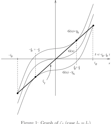
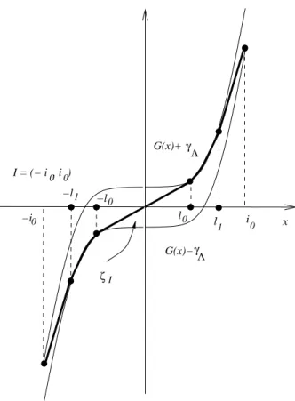
The pictures below illustrate the cases l0 = l1 and l0 < l1 appearing in the
coincidence set, where I is of the form (−i0, i0) containing (−l1, l1).
−l = −l
0 1
l = l
0 1
Λ G(x)+
G(x)
ζ I
x
γΛ
γ G(x) −
I =(−i , i )
0 0
i −i
0 0
G(x)+
G(x)− −i
γ
γ
ζI
Λ Λ
0
−l0 −l 1
l0 l
1 i0 x
0 0
I = (− i , i )
Figure 2: Graph of ζI (case l0 < l1)
Indeed, if there existedζI, a solution to (5.17) such that EI(ζI)<EI(ξI),
then this indicates that ξ is not a solution to (5.10), which is not possible. We have to justify possibility of taking the boundary conditions in the definition ofDI. We know that ξ is a solution to the obstacle problem (5.10)
and (−∞,−l0)∪(l0,∞) is the coincidence set. Using the argument of the
proof of [GR1, Proposition 2.5], [GR2, Proposition 3.2] one can show that
ξ|(−∞,−l0] = γΛ and ξ|[l0,∞) = −γΛ. Thus, ξ restricted to each connected
component of the I\[−l0, l0] is constant.
Let us now calculate Λσ
W. For points of the coincidence set, it is clear
that Λσ
W =σ as desired. Let us consider interval [−l0, l0]. By the definition,
see (2.5), Λσ
W = dxdζχlχr,I, where ζχlχr,I is a solution to the following obstacle problem,
where Z(x) = Rx
0 σ(t, s)ds and for [−l0, l0], we have χl= +1 =χr,
K++Z ={ω ∈H1 : Z(x)−γΛ≤ω(x)≤Z(x)+γΛ, x∈[−l0, l0], ω(±l0) =Z(±l0)±γΛ}.
Since the boundary conditions in KZ
++ are that of D[−l0,l0], we immediately
conclude by previous considerations that ζ defined by Z−ξ is the solution to (5.18). Hence, Λσ
W =σ− ∂x∂ξ.
After these preparation, we may check that a variational solution is a viscosity solution. First, we shall see that d is a supersolution. For this purpose we take a test functionϕ∈AP(Q) such thatd−ϕattains a minimum
at (x0, t0), where t0 ∈(0, T). We have to show that
ϕt−ΛσW ≥0. (5.19)
Inequality (5.19) (and (5.22) below) is to be checked at each point. We have to consider two cases for the interfacial curves: (a) the free boundary
l0 is a tangency curve (b) the free boundary l0 is a matching curve and the
tangency condition is violated.
In the course of proving (5.19) we will consider three cases separately: (i) |x0|> l0(t0), (ii) |x0| ∈[0, l0(t0)), (iii)|x0|=l0(t0).
We begin with (i). Since we assumed thatd0 ∈C1, we know (see Theorem
5.3 or Theorem 5.5) that at (x0, t0) function d is differentiable. Hence for
ϕ(x, t) =f(x) +g(t) with d−ϕ ≥0 in a neighborhood of (x0, t0) we have
dx(x0, t0) =f′(x0), dt(x0, t0) = g′(t0).
Due to Definition 2.10 we have Λσ
W(ϕ) =σ = ΛσW(d). As a result,
0 = dt−σ =g′−ΛσW(ϕ) = ϕt−ΛσW(ϕ),
as desired.
Now we look at (ii). The argument depends on the type of the interfacial curve l0. Let us first assume that l0 is tangency curve.
In the considered case d is also differentiable at (x0, t0). If ϕ is a test
function such that d−ϕ attains its minimum at (x0, t0), then
dx(x0, t0) = 0 =f′(x0), dt(x0, t0) = g′(t0).
Since f ∈ C2
P(Ω), we immediately see that I = R(f, x0), the faceted region
of ϕ at (x0, t0), must contain [−l0, l0]. Let us suppose that ξI is the solution
to