Knot Theory ~

Richard H. Crowell Ralph H. Fox

r'

Knot Theory _~

~ ~

Sf l.O

[jfl ~ &

lArJ _~

Springer-Verlag I

New York I kiddhcrg Berlin I

R. H. Crowell

Department of l\:1athematics Dartmouth College

Hanover, New Hampshire 03755

Editorial Board

R. H. Fox

Formerly of Princeton University Princeton, New Jersey

P. R. Halmos

]'ianaging Editor

Department of Mathematics University of California Santa Barbara,

California 93106

F. W. Gehring

Department of :Mathematics University of :Michigan Ann Arbor, J\:1ichigan 48104

C. C. Moore

Department of :Mathematics University of California

at Berkeley

Berkeley, California 94720

AMS Subject Classifications: 20E40,55A05, 55A25, 55A30

Library of Congress Cat.aloging in Publication Data Crowell, Richard H.

Introduction to knot theory.

(Graduate texts in mathematics 57) Bibliography: p.

Includes index.

1. Knot theory. I. Fox, Ralph Hartzler, 1913- joint author. II. Title. III. Series.

QA612.2.C76 1977 514'.224 77 -22776 ISBN

All rights reserved

No part of this book may be translated or reproduced in any form without written permission from Springer Verlag

©

I B63 by R. H. Crowell and C. Fox Pl'illtodilltho United States of America

IKBN 0:~K7 HO~7~·' Npl'illgOI'-Vn"'Hg Now VOI'I<:

To the memory of

Richard C. Blanchfield and Roger H. Kyle and

RALPH H. FOX

Preface to the Springer Edition

This book was written as an introductory text for a one-semester course and, as such, it is far from a comprehensive reference work. Its lack of completeness is now more apparent than ever since, like most branches of mathematics, knot theory has expanded enormously during the last fifteen years. The book could certainly be rewritten by including more material and also by introducing topics in a more elegant and up-to-date style. Accomplish- ing these objectives would be extremely worthwhile. However, a significant revision of the original \vork along these lines, as opposed to \vriting a new book, would probably be a mistake. As inspired by its senior author, the late Ralph H. Fox, this book achieves qualities of effectiveness, brevity, elementary character, and unity. These characteristics \vould l:?e jeopardized, if not lost, in a major revision. As a result, the book is being republished unchanged, except for minor corrections. The most important of these occurs in Chapter III, where the old sections 2 and 3 have been interchanged and somewhat modified. The original proof of the theorem that a group is free if and only if it is isomorphic to

F[d]

for some alphabet

d

contained an error, which has been corrected using the fact that equivalent reduced words are equal.

I would like to include a tribute to Ralph Fox, who has been called the father of modern knot theory. He was indisputably a first-rate mathematician of international stature. More importantly, he was a great human being. His students and

othe~

friends respected him, and they also loved him. This edition of the book is dedicated to his memory.

Richard H. Cro\vell Dartmouth College

1977

Preface

Knot theory is a kind of geometry, and one whose appeal is very direct hecause the objects studied are perceivable and tangible in everyday physical space. It is a meeting ground of such diverse branches of mathematics as group theory, matrix theory, number theory, algebraic geometry, and differential geometry, to name some of the more prominent ones. It had its origins in the mathematical theory of electricity and in primitive atomic physics, and there are hints today of new applications in certain branches of

(~hemistry.1

The outlines of the modern topological theory were worked out

hy

Dehn, Alexander, Reidemeister, and Seifert almost thirty years ago. As a

HU

bfield of topology, knot theory forms the core of a wide range of problems dealing with the position of one manifold imbedded within another.

This book, which is an elaboration of a series of lectures given by Fox at Haverford College while a Philips Visitor there in the spring of 1956, is an attempt to make the subject accessible to everyone. Primarily it is a text- hook for a course at the junior-senior level, but we believe that it can be used with profit also by graduate students. Because the algebra required is not the familiar commutative algebra, a disproportionate amount of the book is given over to necessary algebraic preliminaries. However, this is all to the good because the study of noncommutativity is not only essential for the (Ievelopment of knot theory but is itself an important and not overcultivated field. Perhaps the most fascinating aspect of knot theory is the interplay h(\tween geometry and this noncommutative algebra.

For the past ,thirty years Kurt Reidemeister's Ergebnisse publication A''fI,otentheorie has been virtually the only book on the subject. During that

f.inH~

many important advances have been made, and moreover the combina- (.ol'ial point of view that dominates K notentheorie has generally given way to a strictly topological approach. Accordingly, we have elnphasized the f,opological invariance of the theory throughout.

rrlH're is no doubt whatever in our minds but that the subject centers nround the coneepts: knot group, Alexander matrix, covering space, and our

pn'S('1l

taLiof} is faithful to this point of vie\\!. We regret that, in the interest

of

k('('ping thp rnatprial at as (·lernentary a lev('1 as possibl(\ we did not

;1If.rodu('('

and tnak(\

s.vst('n}at,i(~

lise of eov(,l'ing

spa(~('

th('ory, How(\v(\r, had

W('

dotH' so, this book

would

have'

lH'('OUI<' UIU(,1t

long(' .. ,

InOI'('

difli(, .. lt, and

I 11.1.. FI·i~..wlt/l.lld It;,\V"N~IC·I'IIIIlIl."('h4·IIIIC·IlI'l'01'0lugy,".I . .11ll.('htOIll.8m·.,X:~ (IHHI)

viii

PREFACE

presumably also more expensive. For the mathematician with some maturity, for example one who has finished studying this book, a survey of this central core of the subject may be found in Fox's "A quick trip through knot theory"

(1962).1

The bibliography, although not complete, is comprehensive far beyond the needs of an introductory text. This is partly because the field is in dire need of such a bibliography and partly because we expect that our book will be of use to even sophisticated mathematicians well beyond their student days.

To make this bibliography as useful as possible, we have included a guide to the literature.

Finally, we thank the many mathematicians who had a hand in reading and criticizing the manuscript at the various stages of its development.

In particular, we mention Lee Neuwirth,

J.

van Buskirk, and R.

J.

Aumann, and two Dartmouth undergraduates, Seth Zimmerman and Peter Rosmarin.

We are also grateful to David S. Cochran for his assistance in updating the

bibliography for the third printing of this book.

Contents

Prerequisites.

Chapter I Knots and Knot Types

1. Definition of a knot 2. Tame versus wild knots.

3. Knot projections

4.,Isotopy type, amphicheiral and invertible knots

3 5 6 8

Chapter IT The Fundamental Group

Introduction . I. Paths and loops

2. Classes of paths and loops 3. Change of basepoint

4. Induced homomorphisms of fundamental groups 5. :Fundamental group of the circle

13 14 15 21 22 24

Chapter m The Free Groups

Introduction . :11

1. The free group F[d'] :11

2. Reduced words :12

:1- Free groups :If>

Chapter IV Presentation of Groups

Introduction.

I. Development of the presentation concept . 2. Presentations and presentation types :1. 'rhe Tietze theorem

4. Word subgroups and the associatedhomomorphiRm~.

!). Free abel ian groups

Chapter V Calculation of Fundamental Groups

Intl'oduction .

I. ItptntetionH and d('forrnat.ions

~. Ilornotop.v typo

:1. 'I'hp van K,unppft tht'on'rJl

X CONTENTS

Chapter VI Presentation of a Knot Group

Intl'oduction .

1. 'rhe over and under presentations

2. 'rhe over and under presentations, continued 3. 'rho Wirtinger presentation

4. Examples of presentations

5. Existence of nontrivial knot types .

Chapter VII • The Free Calculus and the Elementary Ideals

Introduction . 1. The group ring 2. The free calculus 3. The Alexander matrix 4. The elementary ideals

72 72

78

86

87 90

94 94 96 100 101

Chapter VIII The Knot Polynomials

Introduction .

1. The abelianized knot group

2. The group ring of an infinite cyclic group.

3. The knot polynomials

4. Knot types and knot polynomials .

110 I I I 113 119 123

Chapter IX Characteristic Properties of the Knot Polynomials

Introduction .

1. Operation of the trivializer 2. Conjugation .

3. Dual presentations .

Appendix I. Differentiable Knots are Tame Appendix II. Categories and groupoids

Appendix III. Proof of the van Kampen theorem.

Guide to the Literature Bibliography

Index

134 134 136 137

147 153 156 161 165 178

Prerequisites

For an intelligent reading of this book a knowledge of the elements of 1110dern algebra and point-set topology is sufficient. Specifically, we shall assume that the reader is familiar with the concept of a function (or mapping) and the attendant notions of domain, range, image, inverse image, one-one, onto, composition, restriction, and inclusion mapping; with the concepts of equivalence relation and equivalence class; with the definition and elementary properties of open set, closed set, neighborhood, closure, interior, induced topology, Cartesian product, continuous mapping, homeomorphism, eonlpactness, connectedness, open cover(ing), and the Euclidean n-dimen-

~ional

space Rn; and with the definition and basic properties of homomor- phism, automorphism, kernel, image, groups, normal subgroups, quotient groups, rings, (two-sided) ideals, permutation groups, determinants, and Inatrices. These matters are dealt with in many standard textbooks. 'Ve may, for example, refer the reader to A. H. Wallace, An Introduction to Algebraic 'Fopology (Pergamon Press, 1957), Chapters I, II, and III, and to G. Birkhoff and S. MacLane, A Survey of Modern Algebra, Revised Edition (The Mac- l}lillan Co., New York, 1953), Chapters III, §§1-3, 7,8; VI, §§4-8, 11-14; VII,

~5;

X, § §1, 2; XIII, §§1-4. Sonle of these concepts are also defined in the index.

In Appendix I an additional requirement is a knowledge of differential and integral calculus.

l^l

he usual set theoretic symbols

E, c, ~,

=,

U, (1,

and - are used. For the inclusion symbol we follow the common convention: A

c

B means that

1)E B

whenever pEA. For the image and inverse image of A under f we write either fA andf

-1

A, or f(A) and! -l(A). For the restriction off to A we writef I

A,

and for the composition of two mappings!:

X ~

Y and g:

Y~Z

wo write gf.

When several mappings connecting several sets are to be considered at the

~alne

time, it is convenient to display them in a (mapping) diagram, such as

f g

X~y~Z

~1/·

I

r

('(l,('h eh'J)\('IlL in('Hell ~('L di~play('dill a dingl'atll Il:,s aLIno~LOl\(' illlag(' ..1(,- In('IIt, in allY giv('J} :..·wL ofLIlt, di:l,grnJ)l, t,lle' dia,L!;ralll is ~aid t,o I... ("oll8;:·d('II'.

2 PREREQUISITES

Thus the first diagram is consistent if and only if gf == I andfg == I, and the second diagram is consistent if and only if bf ==

a

and cg == b (and hence cgf == a).

The reader should note the following "diagram-filling" lemma, the proof of which is straightforward.

If h: G

-+

Hand k: G

-+

K are homomorphisms and h is onto, there exists a (necessarily unique) homomorphism f: H

-+

K making the diagram

G

/~

H f ) K

consistent if and only if the kernel of h is contained in the kernel of k.

CHAPTER I

Knots and Knot Types

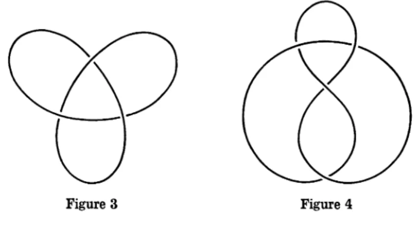
1. Definition of a knot. Almost everyone is familiar with at least the simplest of the common knots, e.g., the overhand knot, Figure 1, and the figure-eight knot, Figure 2. A little experimenting with a piece of rope will convince anyone that these two knots are different: one cannot be trans- formed into the other without passing a loop over one of the ends, i.e.,without

"tying" or "untying." Nevertheless, failure to change the figure-eight into the overhand by hours of patient twisting is no proof that it can't be done.

The problem that we shall consider is the problem of showing mathematically that these knots (and many others) are distinct from one another.

Figure 1 Figure 2

Mathematics never proves anything about anything except mathematics, and a piece of rope is a physical object and not a mathematical one. So before worrying about proofs, we must have a mathematical definition of what a knot is and another mathematical definition of when two knots are to be considered the same. This problem of formulating a mathematical model arises whenever one applies mathematics to a physical situation. The defini- tions should define mathematical objects that approximate the physical objccts under consjderation as closely as possible. The model may be good or had according as the correspondence between mathematics and reality is

good

or bad. There is, however, no way to prove (in the mathematical sense,

and it

is probably only in this sense that thc word has a precisc meaning) that

t.lH~ rnathclnatieal definitions df'HCrihc the physical situatioJl pxaet.ly.

()hviou~·dy,t.he figure-eight knot can be tra.nsf()rrr}(~d into t.h(~ oVPf'han<!

IUlot, hytying and 1Illt.ying in fa('t all kJlOt.Han~('qllival('nt, if UliH olH'raLion iHallow('d. 'rhUHtyingand unt.yingtllllHt,IH'pl'ohihif,('d('iLlIe'"in f,J .. ,d('liniLion

.J

J{NOTS AND KNOT TYPES

Chap. I

of

when two knots are to be considered the same or from the beginning in the v('ry definition of what a knot is. The latter course is easier and is the one

W(~

shall adopt. Essentially, we must get rid of the ends. One way would be to prolong the ends to infinity; but a simpler method is to splice them together.

A(~cordingly,

we shall consider a knot to be a subset of 3-dimensional space whieh is homeomorphic to a circle. The formal definition is: K is a knot if there

(~Xist8

a homeomorphism of the unit circle

C

into 3-dimensional space R3 whose image is K. By the circle 0 is meant the set of points

(x,y)

in the plane 112 which satisfy the equation

x²

+

y2 ===

I.

rrhe overhand knot and the figure-eight knot are now pictured as in Figure :l and Figure 4. Actually, in this form the overhand knot is often called the clover-leaf knot. Another common name for this knot is the trefoil. The figure- eight knot has been called both the four-knot and Listing's knot.

Figure 3 Figure 4

We next consider the question of when two knots K

_I

and

K₂

are to be con- sidered the same. Notice, first of all, that this is not a question of whether or not

K_I

and

K₂

are homeomorphic. They are both homeomorphic to the unit circle and, consequently, to each other. The property of being knotted is not an intrinsic topological property of the space consisting of the points of the knot, but is rather a characteristic of the way in which that space is imbedded in R3. Knot theory is a part of 3-dimensional topology and not of I-dimensional topology. If a piece of rope in one position is twisted into another, the deformation does indeed determine a one-one correspondence between the points of the two positions, and since cutting the rope is not allowed, the eorrespondence is bicontinuous. In addition, it is natural to think

()rtl)(~

rnotioll of

the

I'ope as

aeeornrani(~dby

a nlotiotl of the surrounding

ail' nlol('('lIlps_whi(~hthllsdet('rrni'H's a hi('olltinuolls ')('f'llllltation of

the

pointR of spa('('. 'rlli:--t pi(,tun' ~·nlgg('HLHt.11(' d('filliLion: 1\1l0LHA'I and A':!^al'('()(Inina/tlll

ifU1('f'(' ('xiHL~4^it. ltortlC'Onl()l'pltiHrn of /{l Ollf,o if.:-wlf \Vlli(,11 rnapH /\', ollLo /\''!..

Sect. 2

TAME VERSUS WILD KNOTS

5 It is a triviality that the relation of knot equivalence is a true equivalence relation. Equivalent knots are said to be of the same type, and each equiva- lence class of knots is a knot type. Those knots equivalent to the unknotted circle

x

2 + y2 = I,

Z

= 0, are called trivial and constitute the trivial type.

¹

Similarly, the type of the clover-leaf knot, or of the figure-eight knot is defined as the equivalence class of some particular representative knot. The informal statement that the clover-leaf knot and the figure-eight knot are different is rigorously expressed by saying that they belong to distinct knot types.

2. Tame versus wild knots. A polygonal knot is one which is the union of a finite number of closed straight-line segments called edges, whose endpoints are the vertices of the knot. A knot is tame if it is equivalent to a polygonal knot; otherwise it is wild. This distinction is of fundamental importance. In fact, most of the knot theory developed in this book is applicable (as it stands) only to tame knots. The principal invariants of knot type, namely, the ele- mentary ideals and the knot polynomials, are not necessarily defined for a wild knot. Moreover, their evaluation is based on finding a polygonal repre- sentative to start with. The discovery that knot theory is largely confined to the study of polygonal knots n1ay come as a surprise-especially to the reader who approaches the subject fresh from the abstract generality of point-set topology. It is natural to ask what kinds of knots other than polygonal are tame. A partial answer is given by the following theorcln.

(2.1)

If a knot parametrized by arc length is of class

0¹

(i.e., is continuously differentiable), then it is tame.

A proof is given in Appendix I. It is complicated but straightforward, and it uses nothing beyond the standard techniques of advanced calculus. More explicitly, the assumptions on

K

are that it is rectifiable and given as the image of a vector-valued function p(s)

=

(x(s), y(s), z(s)) of arc length s with con- tinuous first derivatives. Thus, every sufficiently smooth knot is tame.

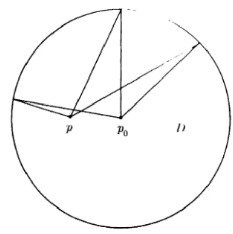
It is by no means obvious that there exist any wild knots. For example, no knot that lies in a plane is wild. Although the study of wild knots is a corner of knot theory outside the scope of this book, Figure 5 gives an example of a knot known to be wild.

²

This knot is a remarkable curve. Except for the faet that the nurnber of loops increases without limit while their size decreases without lirnit (as is indicated in the figure by the dotted square about

p),

the

- - - -

I 1\lly kilo!, wlli('11 IiI'S ill a plalH' is IllH'I'So'-:/l.l'ilyI rivill,1. T}lis i.,-:a \vl'lI-kIlOWIialld dl'Pp Illl'on'lllorplll,1I11topolog,\. _~lln:\. II.!\;I'Wlllllll. /f//f'/IIf'/lfsfd I/'f' 'I'O!J()/()!lI/(d!'/f1lu"I...,'('lsfd

/·()"lIls. ~lll'oll(ll\(liIIOII('lllldll'idgl' (l/livl\l':--lity 1'!'llsH. (1ll.lllhridg(l. I!~;d).p. J7:L .~ I:. II. Il·ll~."\ /:1'111/1,,1\11'"'' ~llIq"I'('Io;";l·d (1111'\'1'." .l/lllltl....f~/ .\1/(I/,III/.{II,.('... \'01. :)() (1!.I!q. p,.. :!t;I.:.!n,r>.

K NO'l'H AND KNOT TYPES

Chap. I

Figure 5

knot could obviously be untied. Notice also that, except at the single point p, it is as smooth and differentiable as we like.

3. Knot projections. A knot

K

is usually specified by a projection; for example, Figure 3 and Figure 4 show projected images of the clover-leaf knot and the figure-eight knot, respectively. Consider the parallel projection

defined by f!JJ(x,y,z)

==

(x,y,O). A point p of the image f!JJK is called a multiple point if the inverse image f!JJ-lp contains more than one point of K.

The order of p

E

f!JJK is the cardinality of (f!JJ-1p) n K. Thus, a double point is a multiple point of order 2, a triple point is one of order 3, and so on.

Multiple points of infinite order can also occur. In general, the image f!JJ

K

may be quite complicated in the number and kinds of multiple points present.

It is possible, however, that

K

is equivalent to another knot whose projected image is fairly simple. For a polygonal knot, the criterion for being fairly simple is that the knot be in what is called regular position. The definition is as follows: a polygonal knot K is in regular position if: (i) the only multiple points of

K

are double points, and there are only a finite number of them;

(ii) no double point is the image of any vertex of

K.

The second condition insures that every double point depicts a genuine crossing, as in Figure 6a.

The sort of double point shown in Figure 6b is prohibited.

FiKUl'e

Oa

Fif{ure

6b

Sect. 3

KNOT PROJECTIONS 7

Each double point of the projected image of a polygonal knot in regular position is the image of two points of the knot. The one with the larger z-coordinate is called an overcrossing, and the other is the corresponding undercrossing.

(3.1) Any polygonal knot K is equivalent under an arbitrarily small rotation of R3 to a polygonal knot in regular position.

Proof. The geometric idea is to hold K fixed and move the projectIon.

Every bundle (or pencil) of parallel lines in R3 determines a unique parallel projection of R3 onto the plane through the origin perpendicular to the bundle.

We shall assume the obvious extension of the above definition of regular position so that it makes sense to ask whether or not

K

is in regular position with respect to any parallel projection. It is convenient to consider R3 as a subset

³

of a real projective 3-space P3. Then, to every parallel projection we associate the point of intersection of any line parallel to the direction of projection with the projective plane p2 at infinity. This correspondence is clearly one-one and onto. Let Q be the set of all points of p2 corresponding to projections with respect to which K is not in regular position. We shall show that Q is nowhere dense in P2. It then follows that there is a projection 9

₀

with respect to which K is in regular position and which is arbitrarily close to the original projection f!JJ along the z-axis. Any rotation of R3 which transforms the line

&>0-1

(0,0,0) into the z-axis will suffice to complete the proof.

In order to prove that Q is nowhere dense in p2, consider first the set of all straight lines which join a vertex of K to an edge of K. These intersect p2 in a finite number of straight-line segments whose union we denote by Q1' Any projection corresponding to a point of p2 - Q 1 must obviously satisfy con- dition (ii) of the definition of regular position. Furthermore, it can have at most a finite number of multiple points, no one of which is of infinite order.

It remains to show that multiple points of order

n

2 3 can be avoided, and this is done as follows. Consider any three mutually skew straight lines, each of which contains an edge of K. The locus of all straight lines which intersect these three is a quadric surface which intersects p2 in a conic section.

(See the reference in the preceding footnote.) Set Q

₂

equal to the union of all such conics. Obviously, there are only a finite number of them. Furthermore, the image of K under any projection which corresponds to some point of p2 - (Ql

U

Q2) has no multiple points of order

n

2 3. We have shown that

'rhus Q is a subset ofQl

U

Q2' whieh is nowhere dense in

]J2.

This

compl(~teH

the proof of

(;~.I). \ '/

:J FOI'all W'('OIIlILof111(\(·olH'opL:-t lI:-tod ill l.hiN proof',:-t(\On. Vohloll alld .J.\V. YOIIIIJ.~, /Jrojf'('li",> (/('011/.('11'.'/ (~illll /tlld ('olllpaIlY. Bw·d,()Il, lVlaH'''IlH'hll:-l(\LLH, IHIO). Vol. I pp. II,

~~~H, :~OI.

J{NO'I'H AND KNOT TYPES

Chap. I

'rhlls,

every tame knot is equivalent to a polygonal knot in regular position.

'ria

is

j~tet

is the starting point for calculating the basic invariants by which diff('rent knot types are distinguished.

4. Isotopy type, amphicheiral and invertible knots. This section is not a prerequisite for the subsequent development of knot theory in this book.

'I'he

contents are nonetheless important and worth reading even on the first time through.

Our definition of knot type was motivated by the example of a rope in motion from one position in space to another and accompanied by a displace- ment of the surrounding air molecules. The resulting definition of equivalence of knots abstracted from this example represents a simplification of the physical situation, in that no account is taken of the motion during the transi- tion from the initial to the final position. A nlore elaborate construction, which does model the motion, is described in the definition of the isotopy type of a knot. An isotopic deformation of a topological space X is a family of homeolTIorphisms ht, 0

S

t

S

1, of X onto itself such that h

_o

is the identity, i.e., ho(p) = p for all p in X, and the function H defined by H(t,p) = ht(p) is simultaneously continuous in

t

and

p.

This is a special case of the general definition of a deformation which will be studied in Chapter V. Knots K

₁

and K

2

are said to belong to the same isotopy type if there exists an isotopic deformation {ht} of R3 such that h1K

₁

= K

₂•

'l'helettert is intentionally chosen to suggest time. Thus, for a fixed point p

E

R3, the point ht(p) traces out, so to speak, the path of the molecule originally at

p

during the motion of the rope from its initial position at K

₁

to K

₂.

Obviously, if knots K

_I

and K

₂

belong to the same isotopy type, they are equivalent. The converse, however, is false. The following discussion of orientation serves to illustrate the difference between the two definitions.

Every homeomorphism h of R3 onto itself is either orientation preserving or orientation reversing. Although a rigorous treatment of this concept is usually given by homology theory,4 the intuitive idea is simple. The homeo- morphism

h

preserves orientation if the image of every right (left)-hand screw is again a right (left)-hand screw; it reverses orientation if the image of every right (left)-hand screw is a left (right)-hand screw. The reason that there is no other possibility is that, owing to the continuity of

h,

the set of points of R3 at which the twist of a screw is preserved by

h

is an open set and the same iH true of the set of points at "\\rhich the twist is reversed. Since

h

is a homeo-

I /\ 110llll'OIJ10I'pllislllk0("thon-sphe!'o~""'n,n 1, ont.o itself isorientation preservingor

1'I·,'(·,....^unf/JI.(·(·ol'dillgliS t11('iSOlllO!'pllislllk*: l'IIU"l'lI) ~11,,(8¹¹)isOJ'isnot tho identity. Lot

I ...' " 1.'''1...J: I : 1)(' till'Oill'!loillt (·()1I1pw·t.ifj(·aLiol\ ort I\(, !'('al(larf,("..;jan_JI-spa~oUn. Any

11l1l1lt'tllll()I'I'III'·HlIIt Ill' N"UllIn ils(·If' lias a lIlli'llII' (1:\1('IlLioll ton 110l1H'olllorpllislIl k of

j ... " N"t J: ' :11ItlH 11'14·11 dl,lilltld II,\' k

II.'"

It IIlld 1.'(,/,) '/1. 'I'll(II.Ii is o"//'II/a//on

, " .. ." " •. r,I" ',',,'ill11t'('lIl'dlll~~11:1I, I : III'III/If IIIIH/I P"(':';4'1'\'IIIJ~HI'1'l1\·(\1·:-\1111-~.

Sect. 4

ISOTOPY TYPE, AMPHICHEIRAL AND INVERTIBLE KNOTS 9

morphism, every point of R3 belongs to one of these two disjoint sets; and since R3 is connected, it follows that one of the two sets is empty. The com- position of homeomorphisms follows the usual rule of parity:

hI

h₂

h

₁

h

₂

preserving preserving preserving reversing preserving reversing preserving reversing reversing reversing reversing preserving

Obviously, the identity mapping is orientation preserving. On the other hand, the reflection

(x,y,z) ~(x,y,-z)

is orientation reversing. If

h

is a linear transformation, it is orientation preserving or reversing according as its determinant is positive or negative. Similarly, if both h and its inverse are 0

¹

differentiable at every point of R3, then h preserves or reverses orientation according as its Jacobian is everywhere positive or

everywher~

negative.

Consider an isotopic deformation {ht} of R3. The fact that the identity is orientation preserving combined with the continuity of H(t,p)

===

ht(p), suggests that h

_t

is orientation preserving for every t in the interval 0

s;::

t s 1.

This is true.s As a result, we have that a necessary condition for two knots to be of the same isotopy type is that there exist an orientation preserving homeomorphism of R3 on itself which maps one knot onto the other.

A knot K is said to be amphicheiral if there exists an orientation reversing homeomorphism h of R3 onto itself such that hK == K. An equivalent for- mulation of the definition, \\t'hich is more appealing geometrically, is provided by the following lemma. By the mirror irnage of a knot K we shall mean the image of

K

under the reflection f!l defined by

(x,y,z) _~(x,y,-z).

Then,

(4.1)

A knot K is amphicheiral

~f

and only if there exists an oriental£on preserving homeomorphism of R3 onto itself which maps K onto its m1'rror

iUUlf/P.

Proof. If K is amphicheiral, the composition /Jih is orientation

pr(~s('rvillg

and maps

K

onto its mirror image. Conversely, if

h'

is an orientation }>n's('rv- ing homeomorphism of R3 onto itself which maps

K

onto its mirror irnag(',

Lltt'

composition

_~h'

is orientation reversing and

_(/~h')K

==

K. \

j

It is not hard to show that the figure-eight knot is amphi('h('iral.

rrhe

('xpprimental approach is th<: best; a rope \\'hich has been tied as a figun'-('ight and

th~n

spliced is quite <:asily twist<:d into its rnirror image.

Thp

0pt'ratioll iH illustratpd in

Figun~

7. On the other hand, the'

('l()v('r-h~af

knot is

not

arnphi-

fl Any i~otopi(' d ..fol'rllnt ion

:h

t }, . . . I" I, of 1lin ('Hrtt'~UUl /'I.-spa(',' Uri (h·finit.nly

p4)~snS~t·~a Ilni'llln('xtl'n~i()n10au i~ot()pit'dt·forrllutlOll {kd,o· I · I,oft lin 1/ '..qdl4\l'n 1\''',i.t-., k_tI^{Nil h"} und"',(,1) IJ. Fill'I'lll'hI, thnhOll,f'/1I110l'Jdll"';1I1k,I"';Jlflfllfdopll'to thn ul,·util.\" ulld YII IlllI IlId'lI'l-d I...;OIIlIl!'"III ...,1I (k,). Oil /1,,(,\'11) I~;thf' Idfllddy. I" 11IIIowH tlIlLl.Itt IY 1I1'If'IdHllflli111"""'1'\III~~IIII'H i l I III 0 I ' I.

U·"'.·f·

HI',11 1II01llotll L)

10 KNOTS AND KNOT TYPES

Chap.

I

(1)

(4)

(2)

(5)

Figure 7

(3)

(6)

cheiral. In this case, experimenting with a piece of rope accomplishes nothing except possibly to convince the skeptic that the question is nontrivial.

Actually, to prove that the clover-leaf is not amphicheiral is hard and requires fairly advanced techniques of knot theory. Assuming this result, however, we have that the clover-leaf knot and its mirror image are equivalent but not of the same isotopy type.

It is natural to ask whether or not every orientation preserving homeo- morphism f of R3 onto itself is realizable by an isotopic deformation, i.e., gi ven f, does there exist

{h_{t },}

0

_~

t

~

I, such that f ==

h₁1

If the answer were no, we would have a third kind of knot type. This question is not an easy one.

I'fhe answer is, however, yes.

⁶

Just as every homeomorphism of R3 onto itself either preserves or reverses orientation, so does every homeomorphism f of a knot K onto itself. The geometric interpretation is analogous to, and simpler than, the situation in

:~-dirnensional

space. Having prescribed a direction on the knot,fpreserves or

n~verHe~

orientation according as the order of points of K is preserved or re-

v(~J'Hed

under f. A knot K is called invertible if there exists an orientation pre- HnJ'ving horneoInorphisnl h of R3 onto itself such that the restriction h I ^K

iH an Ol'inlltatioll ("Pvol'Hing

honH~olnorphisrn

of K onto itself. Both the c]over-

II(L M. 1⁴'iHllclI·.H()IIl.Ilo(:1'0111'of 11.11 1I01lioolllorpiliHIllH or II Mallifold,"'/'rOIl8(f('''':ons of /hl' :1"11'1'1('(111 fl/fI/hnlJ,(//u·(/l/..,'O('II'/.'/, Vol. H7 (IHHO), pp. IH:C ~~I~.

Sect. 4

ISOTOPY TYPE, AMPHICHEIRAL AND INVERTIBLE KNOTS 11

leaf and figure-eight knots are invertible. One has only to turn them over (cf. Figure

8).

Figure 8

Until recently no example of a noninvertible knot was known. Trotter solved the problem by exhibiting an infinite set of noninvertible knots, one of which is shown in Figure 9.

⁷

Figure 9

EXERCISES

1. Show that any simple closed polygon in R2 belongs to the trivial knot type.

2. Show that there are no knotted quadrilaterals or pentagons. What knot types are

reprcHented by hexagonH? hyHPptag(H1H'~

7II. F. Trot.t.p .. , ..NOllillvnl't.itdn IUlOt.H nxiHt.." '/'o/wl0!l.'l, vol. ~(I BH·I), pp. ~7[) ~HO.

I~ ^I{N()TS AND KNOT TYPES

Chap. I

:L I)(~vise

a method for constructing a table of knots, and use it to find the

f,.'11

knots of not more than six crossings. (Do not consider the question of

Wh<,UH'T'

these are really distinct types.)

.1. I

)('termine by experilnent which of the above ten knots are obviously H.lllphi(·hciral, and verify that they are all invertible.

£).

Nhow that the number of tame knot types is at most countable.

n. (Brunn) Show that any knot is equivalent to one whose projection has at, t}lost one multiple point (perhaps of very high order).

7.

(1-'ait) A polygonal knot in regular position is said to be alternating

if

the undercrossings and overcrossings alternate around the knot. (A knot type is called alternating if it has an alternating representative.) Show that if

I{

is any knot in regular position there is an alternating knot (in regular position) that has the same projection as

K.

H.

Show that the regions into which R2 is divided by a regular projection ean be colored black and white in such a way that adjacent regions are of opposite colors (as on a chessboard).

B.

Prove the assertion made in footnote 4 that any homeomorphism h of Rn onto itself has a unique extension to a homeomorphism k of sn == Rn

U

{oo}

011

to itself.

10.

Prove the assertion made in footnote 5 that any isotopic deformation

{ht},O :::;: t :::;: 1, of Rn possesses a unique extension to an isotopic deformation

{k

_t},

0 :::;: t :::;: 1, of sn. (Hint: Define F(p,

t)

==

(ht(p),t),

and use invariance of

dornain to prove that F is a homeomorphism of Rn

X

[0, IJ onto itself.)

CHAPTER

II

The Fundamental Group

Introduction. Elementary analytic geometry provides a good example of the applications of formal algebraic techniques to the study of geometric concepts. A similar situation exists in algebraic topology, where one associates algebraic structures with the purely topological, or geometric, configurations.

The two basic geometric entities of topology are topological spaces and con- tinuous functions mapping one space into another. The algebra involved, in contrast to that of ordinary analytic geometry, is what is frequently called modern algebra. To the spaces and continuous maps between them are made to correspond groups and group homomorphisms. The analogy with analytic geometry, ho\vever, breaks down in one essential feature. Whereas the coordinate algebra of analytic geometry completely reflects the geometry, the algebra of topology is only a partial characterization of the topology. rrhis means that a typical theorem of algebraic topology will read: If topological spaces

X

and Yare homeomorphic, then such and such algebraic conditions are satisfied. The converse proposition, however, will generally be false. Thus, if the algebraic conditions are not satisfied, we know that

X

and Yare topo- logically distinct. If, on the other hand, they are fulfilled,

we

usually can conclude nothing. The bridge from topology to algebra is almost always a one-way road; but even with that one can do a lot.

One of the most important entities of algebraic topology is the fundamental group of a topological space, and this chapter is devoted to its definition and elementary properties. In the first chapter we discussed the basic spaces and continuous maps of knot theory: the 3-dimensional space R3, the knots them- sclves, and the homeomorphisms of R3 onto itself which carry one knot onto another of the same type. Another space of prime importance is the c01nple- /Jnentary space R3 - K of a knot K, which consists of all of those points of R3 that do not belong to K. All of the knot theory in this book is a study of the properticH of the fundarnental groups of the cornplerncntary spaces of knots, alld this is ind(\(\d

th(~

('(\lltraJ thetne of the (\ntire

sttbj(~et.

I n this ehapter, Il()\vevpl', thp d(·v(·loptll(·nt of" t.IH· f"ulldarn(,lltal group iN Inad(\

for

all arbitrary topologi('nl Npn(T .\' nud iN illd(·IH'rld('Ilt. of" our lat('r ilppli('atiottN of" t.hn

f'tlr)(laIlH'nt~"

grollp

1,0

I\llof.

UH'ory.

1·( TIII~ FUNDAMENTAL GROUP

Chap. II 1. Paths and loops. A particle moving in space during a certain interval ()f

f,ill)(~

describes a path. It will be convenient for us to assume that the motion IU'gills at time t == 0 and continues until some stopping time, which may differ

1'01'

different paths but may be either positive or zero. For any two real num-

Iwl's

:c

and

y

with

x :::;:y,

we define

[x,y]

to be the set of all real numbers t NH,Lisfying x :s: t :s: y.

A

path a in a topological space

X

is then a continuous .napping

a:

[0,11

a

II]

-+X.

'I'IH'

number II a 11 is the stopping time, and it is assumed that II a II

~

O. The

po

in

t~

a(

0)

and a(" a \I) in

X

are the initial point and terminal point, respec- ti vely, of the path a.

It is essential to distinguish a path a from the set of image points a(t) in

X

visited during the interval [0,11

a

II]. Different paths may very well have the saIne set of image points. For example, let

X

be the unit circle in the plane, gi ven in polar coordinates as the set of all pairs

(r,O)

such that

r

== 1. The two paths

a(t) == (1,t), b(t) == (1,2t),

o :::;: t :s: 27T,

o :::;: t :::;: 27T,

are distinct even though they have the same stopping time, same initial and

t(~J'rninal

point, and same set of image points. Paths a and b are equal if and only

if

they have the same domain of definition, i.e., II a \I == II b II, and, if for

(~v(~ry

t in that domain, a(t) == b(t).

Con...

~ider

any two paths a and b in X which are such that the terminal point ()f a eoincides with the initial point of b, i.e., a( II a II) == b(O). The product a . b of' the paths

a

and b is defined by the formula

{ a(t),

(a'b)(t)

=

b(t-lIall)'

o :s: t :s: II a II,

II a II :s: t

:S:

II a II + ^{II b} II·

It _i~

obvious that this defines a continuous function, and a · b is therefore a I)ath

in

X. Its stopping time is

II a . b "

=

II a II + " ^b

^II·

\V(~ ernpha~ize

that the product of two paths is not defined unless the terminal ,)() i

11t

of the first is the same as the initial point of the second. It is

0

bvious that

U)(~

three

a~sertions

(i) n'

band

b .c

are defined,

(ii) a' (h .c)

is defined,

(iii) (a· h) .c1:8d(~fin(J,d,

:In'

('qllivalnllt

and

that whenever

one of

thern holdR, the associative lau),

a' (h·

t)

^{(0 .I)) • (.,}

iN

varid.

A

pilthf1 iN ('alle'd :lll idf'lIlil.'lI}(llh, 01'silnply all ide'lltiLy, if if,

has

HLopping

f,iftIe' 1/

(f" (). ' r

hi:-i f,e'rrItiII ()I()g y rc'fie' c. f.:-l UIf' 1"11.f •f, LllJl,f,UIf':-14' f, f)

r

aII idf'IILiL'y

Sect. 2

CLASSES OF PATHS AND LOOPS

15 paths in a topological space may be characterized as the set of all multipli- cative identities with respect to the product. That is, the path e is an identity if and only if e . a

=

a and b· e

=

b whenever e· a and b· e are defined.

Obviously, an identity path has only one image point, and conversely, there is precisely one identity path for each point in the space. We call a path whose image is a single point a constant path. Every identity path is constant; but the converse is clearly false.

For any path a, we denote by a-I the inverse path formed by traversing a in the opposite direction. Thus,

a-I(t) == ^{a(11 a} II - t), o s:: t s:: II a

II.

The reason for adopting this name and notation for a-I will become apparent as we proceed. At present, calling a-I an inverse is a misnomer. It is easy to see that a . a-I is an identity e if and only if a === e.

The meager algebraic structure of the set of all paths of a topological space with respect to the product is certainly far from being that of a group. One way to improve the situation algebraically is to select an arbitrary point

p

in

X

and restrict our attention to paths which begin and end at

p.

A path whose initial and terminal points coincide is called a loop, its common endpoint is its basepoint, and a loop with basepoint p will frequently be referred to as p-based. The product of any two p-based loops is certainly defined and is again a p-based loop. Moreover, the identity path at

p

is a multiplicative identity. These remarks are summarized in the statement that the set of all p-based loops in

X

is a semi-group with identity.

The semi-group of loops is a step in the right direction; but it is not a group.

Hence, we consider another approach. Returning to the set of all paths, we shall define in the next section a notion of equivalent paths. We shall then consider a new set, whose elements are the equivalence classes of paths. The fundamental group is obtained as a combination of this construction with the idea of a loop.

2. Classes of paths and loops. A collection of paths

h_s

in

X,

0 s:: s s:: ^{I, will}

be called a continuous family of paths if

(i) The stopping time"

h_s

II depends continuously on s.

(ii) The function h defined by the formula h(s,t) == hs(t) maps the closed region 0 s:: s s:: ^{1, 0} s:: ^t s:: II

h_s

II continuously into

X.

It should be noted that a function of two variables which is continuous at every point of its domain of definition with respect to each variable is not necessarily continuous in both simultaneously. The function f defined on the unit

Hquare0 <:s .~ I, 0

.< t

<--: 1 by

the formula

/(8,1)

r

^I,

. 8

I

I

I /') ')'

^V8"

^I

^lu

if,';

0,

(If,ll('rwiHC',

IH Tllli~ :FUNDAMENTAL GROUP

Chap. II

is all

('xample. The collection of paths {fs} defined

by

fs(t) == f (s,t) is not, UI('f'('fore, a continuous family.

i\ Ji.rf'd-endpoint family of paths is a continuous family {h _s}' 0

~

s :::;: I,

1411('1.

that hs(O) and hs( II _hs II) are independent of s, i.e., there exist points p and

(I

in .X

Nueh that

hs(O)

== p and hs(11

h

s II) == q for aIls in the interval

0 :::;:

s :::;: I.

'rl)(~

difference between a continuous family and a fixed-endpoint family is illuNtrated below in Figure 10.

h

Figure 10

J.Jet a and b be two paths in the topological space X. Then, a is said to be (Iqnivalent to

b,

written a

^r--I b,

if there exists a fixed-endpoint family

{h_s}'

n . -

8

-< 1, of paths in X such that a == h o ^{and b} == hI'

rrhe relation,-...J is reflexive, i.e., for any path a, we have a ,-...J a, since we may obviollNly define hAt)

==

a(t), 0 :::;;: s

~

I. It

i~

also symmetric, i.e., a,-...J b ilnpJi('N h

~ ^(J"

because we may define ks(t) = h1-s(t). Finally, ,-...J is transitive,

i,p"

a

^,-...J

hand b c::: c irnply a ,-...J c.

1'0

verify the last statement, let us suppose

t.hat.

!Is

alld /(',:> are t.he

fixed-endpoint families exhibiting the equivalences

( ( r - J hand /) ^{r - J ( '} I'('Np(,(~tiv('l'y,rrhCIl the eoJJeetioll

of pathN (f,J defined by

o ",. J,

s I,

Sect. 2

CLASSES OF PATHS AND LOOPS

17 is a fixed-endpoint family proving a

^f"'--J

c. To complete the arguments, the reader should convince himself that the collections defined above in showing reflexivity, symmetry, and transitivity actually do satisfy all the conditions for being path equivalences: fixed-endpoint, continuity of stopping time, and simultaneous continuity in

8

and t.

Thus, the relation

f"'--J

is a true equivalence relation, and the set of all paths in the space

X

is therefore partitioned into equivalence classes. We denote the equivalence class containing an arbitrary path a by [a]. That is, [a] is the set of all paths

b

in X such that a

^,-....J b.

Hence, we have

[a] === [b] if and only if a

^f"'--J

b.

The collection of all equivalence classes of paths in the topological space

X

will be denoted by

r(X).

It is called the fundamental groupoid of X. The definition of a groupoid as an abstract entity is given in Appendix II.

Geometrically, paths a and

b

are equivalent if and only if one can be continuously deformed onto the other in

X

without moving the endpoints.

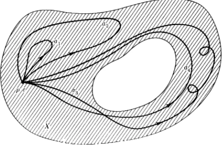
The definition is the formal statement of this intuitive idea. As an example, let X be the annular region of the plane shown in Figure 11 and consider five loops e (identity),

aI'

a

_{2 ,}

a

_{3 ,}

a

₄

in X ^{based at}

p.

We have the following equivalences

a

_l ^f"'--J

a

₂^f"'--J

e, a

₃^f"'--J

a

₄^•

However, it is not true that

Figure 11 shows that certain fundamental properties of X are reflected in the equivalence structure of the loops of

X.

If, for example, the points lying inside the inner boundary of

X

had been included as a part of

X,

i.e., if the

Figure 11

1ft TilIi; FUNDAMENTAL GROUP

Chap. II

1,"1.-

\\'4'1"(' filled in, then all loops based at

p

would have been equivalent to the

,d"ltl!f"v

Joop e. It is intended that the arrows in Figure II should imply that

III 1111'

interval of the variable t is traversed for each

ai'

the image point runs

II Ie HIlid

the circuit once in the direction of the arrow. It is essential that the

,de'll ofa_i

as a function be maintained. The image points of a path do not ''IH'4'ify the path completely; for example, a

₃

=j=. a

₃•

a

₃,

and furthermore, we

ele.

not even have, a

₃~

a

₃•

a

₃.

We shall now show that path multiplication induces a multiplication in the fundamental groupoid

r(X).

As a result we shall transfer our attention from paths and products of paths to consideration of equivalence classes of paths and the induced multiplication between these classes. In so doing, we shall obtain the necessary algebraic structure for defining the fundamental group.

(2.1) For any paths a, a', b, b' in X, if a· b is defined and a

_~

a' and b

~

b', then a' . b' is defined and a' b ,-....; a' . b'.

Proof. If {h

_s}

and {k

_{s }}

are the fixed-endpoint families exhibiting the equivalences a,-....; a' and b

~

b', respectively, then the collection of paths {h

_{s •}

k

_s}

is a fixed-endpoint family which gives a . b

~

a'· b'. We observe, first of all, that the products

h_{s •}k_s'

are defined for every s in

0 S

s

S 1

because

In particular, a' . b' ==

hI .k_I

is defined. It is a straightforward matter to verify that the function

h . k

defined by

(h . k)(s,t) === (h

s · ks)(t), o s s s

I, 0 S t

s II

hs

II + II

^ks

II,

is simultaneously continuous in sand t. Since II h

_{s •}

k

_s

II

⁼⁼

II h

_s /I

+

^/I

k

_s1/

is a continuous function of s, the paths

h_{s •}k_s

form a continuous family. We have

and

so that

{h_{s •}k_s}'

0 s ^s s I, is a fixed-endpoint family. Since

h

o .

^k

o

⁼⁼⁼

a ·

b

and

hI ·

k

_I ===

a' · b' , the proof is complete.

Consider any two paths a and b in X such that a · b is defined. The product of the equivalence classes

[a]

and

[b]

is defined by the formula

[a] . [b] ===[a . b].

Multiplication in

r(X)

is well-defined as a result of

(2.1).

Since all paths belonging to a single equivalence class have the same initial

point and the Harne t~rrninal point, we rnay dpfine

the

initial point

and

t('rminal point, of an ('1(,Tlu'nt ex in r(.X) t,ol)(~ thos(' ofan arbitrary r('pr~~en­

tativ(' pat,lt in (1. 'rtH' prodll(,t rx. .

II

^off,wo('1('ln4'llt,~ rx. and

II

^{ill r(X)} i~ thnn

Sect. 2

CLASSES OF PATHS AND LOOPS

19 defined if the terminal point of

^lI..

coincides with the initial point of fJ. Since the mapping

a~[a]

is product preserving, the associative law holds in

r(X)

whenever the relevant products are defined, exactly as it does for paths.

An element

E

in

r(X)

is an identity if it contains an identity path. Just as before, we have that an element

E

is an identity if and only if

E •lI.. = lI..

and

fJ .

^E

= fJ whenever

E •lI..

and fJ ·

^E

are defined. This assertion follows almost trivially from the analogous statement for paths. For, let

E

be an identity, and suppose that

E •lI..

is defined. Let e be an identity path in

E

and a a represent- ative path in

lI...

Then, e· a = a, and so

E'lI..

=

^lI...

Similarly, f3.

E

= f3.

Conversely, suppose that

^E

is not an identity. To prove that there exists an

^r:J..

such that

^{E •lI..}

is defined and

^{E •}

lI...=I=-

^lI..,

select for

^lI..

the class containing the identity path corresponding to the terminal point of

^E.

Then,

^{E •lI..}

is defined, and, since

^lI..

is an identity,

^{E •r:J..}

=

^E.

Hence, if

^{E •lI..}

=

^r:J..,

the class

^E

is an identity, which is contrary to assumption. This completes the proof. We con- clude that

r(X)

has at least as much algebraic structure as the set of paths in

X.

The significant thing, of course, is that it has more.

(2.2) For any path a in X, there exist identity paths

e₁

and e

₂

such that a · a-I

^r--Je₁

and a-I. a ,-...; e

₂^•

Proof. The paths e

₁

and e

₂

are obviously the identities corresponding to the initial and terminal points, respectively, of a. Consider the collection of paths {h

_{s },}

0 :::;: s

~

1, defined by the formula

{ a(t), hs(t) =

a(2s II a II -

t),

o

~

t :::;: s II a II,

s II a II :::;: ^t

~

2s II a

II·

The domain of the mapping h defined by h(s,t) = hs(t) is the shaded area shown in Figure 12. On the line

t

= 0, i.e., on the s-axis,

h

is constantly equal to

a(O).

The same is true along the line t = 2s II

^a

II. Hence the paths h

_s

form a

('1

/lall

Fig-ure 12

2/1all

THE FUNDAMENTAL GROUP

Chap. II

Ii

x('d-endpoint family. For values of

t

along the horizontal line s == 1, the

rllll(~tionh

behaves like a . a-I. We have

h_o

==

c_i

{ a(t), hI(t) ==

a(2

II

a

II -

t),

( a(t),

- a-I(t - II a

II),

==

(a •

a-1)(t),

o

~t ~

II

a

II,

II a II

~

t

~

2 II a II,

o

~t _~

II a

II,

II

a

II

~

t

~2

II

a

II,

and

the proof that a . a-I

r-J e_i

is complete. The other equivalence may, of

(·()tlr~e,

be proved in the same way, but it is quicker to use the result just proved to conclude that a-I.

(a-I)-I r-J

e

₂.

Since

(a-I)-I

== ^a, the proof is (:ornplete.

(2.3)

For any paths a and

b,

if a

^r-J b,

then a-I

~ b-1 .

Proof. This result is a corollary of

(2.1)

and

(2.2).

We have

()n

the basis of

(2.3),

we define the inverse of an arbitrary element

lI..

in

r(X) hy

the formula

lI..-I

== ^[a-I], for any a in

r:t..

rl'he element

r:t.-I

depends only on

(I.,

and not on the particular representative path a. That is,

(1.,-1

is well-defined. This time there is no misnaming. As a corollary of (2.2), we have

(2.4)

For any

r:t.

in

r(X),

there exist identities

E}

and

E2

such that

(I., • (1.,-1

==

^EI

and

a.-I. a.

==

^E2'

The additional abstract property possessed by the fundamental groupoid

l-'(X)

beyond those of the set of all paths in X is expressed in

(2.4).

We now obtain the fundamental group of

X

relative to the basepoint

p

by defining the exact analogue in

r(X)

of the p-based loops in the set of all paths: Set

7T(X,p)

equal to the subset of

r(X)

of all elements having

p

as both initial and terminal point. The assignment

a~[a]

determines a mapping of the semi·

group of p-based

Ioop~

into 7T(X,p) which is both product preserving and onto.

ft followH that

7T(X,p)

is a semi-group with identity and, by virtue of

(2.4),

we have

(~.r))

'1

^Yhe S()t7T(

X,/»,

lOfJf)ther un:th the1nnltir)Z,icaIiond(~fi'n()d,isa

group. It

i~ by dnfillitiof} U)(~fnndflIJtJ,(lJllal yroll/)l (~l

..\

i'(Jlati'I'() to tllf} !Ja,""fJl){n:ntp.

I TIIlI('Il~lflllllll,rylI11tHtillllill tllplliogy rlll"llllN grollpi~iIT,(X.I'),'1'1\(11'/1i:-:a :-:.l(llllII\(~O of l-~roIlJl:j1I

11(X ./,)./I I .• 'ldl.,d lit., 1""1101III'.\'J,..~l'Cllll':-IIII'X !'l'lnll\p tII I'.'1'1111l'lIl1dllllll'nt,al

l ' r H I I " Iii111.'fil':iI l i l l i '0/ 1114\:H'qlll·IWll.