VI-2-2. Multi-dimensional Scaling method; MDS VI-2-2-1. What is MDS
Purpose of Multi-dimensional Scaling method (MDS) is similar as that of Principle Component Analysis (PCA). MDS and PCA put data in multi-dimensional space for observation of relationship among data. However, forms of given data are different between MDS and PCA. A datum is composed from more than two measurement items in PCA. When we consider average vectors of each measurement item, length of vector is standard deviation, angle between vectors is arccosine, and data can be expressed by linear combinations in multi-dimensional space. Given data in MDS are distance between survey points. Rhetorically, distance means not only physical distance in Euclidean space (orthogonal space). All difference can be recognized as “distance” when it satisfies definition of distance. The definition is
1. Distance from A to B is equal to Distance from B to A
2. Distance from A to C is no longer than sum of distance from A to B and distance from B to C.
However, we consider the distances is Euclidean distance in this explanation for simplification. We learned congruency of triangle in junior high school. We can allocate 3 point on two-dimensional flat. We can add another point in three-dimensional space if we know the distance from the new point to all of the three points on the flat. Generally, the points form delta corn. Of course, they sometimes form plane locus in particular cases.
Similarly, 5 points can allocate in 4-dimansional space. Theoretically, we can allocate all data in n-1-dimensional space at most, when the size of data is n. In reality, obtainable data include limited number of components and most of the dimensions come into the space by error and the space is depressed in the directions of vectors of the component made by error. Neglecting such dimensions, we can allocate all data in limited dimensional space, ideally 2 or 3-dimension. This is a simplest explanation of MDS. A datum has a number of observed measurement items in PCA. We can estimate angle between two vectors of observed value from the correlation efficiency. From the lengths of vectors (standard deviation) and angles among vectors, we can frame multi- dimensional space. This is comparable to proof of congruence of triangles by two lengths and an angle between the sides. For this reason, maximum dimension of the space is 𝑝 when number of observed measurement items is 𝑝. Comparatively, space is fremed only by distance in MDS. This is comparable to proof of congruence of triangle by length of three side. Data form and calculation procedure are different, though purposes of the analyses are the same between MDS and PCA.
MDS is used widely in ecological survey, because we can identify structure of data depending on the difference among data when the difference satisfies the definition of distance. However, we can use MDS in other disciplines.
VI-2-2-1. Calculation of MDS VI-2-2-1-1. Problem setting of MDS
We regularly see result of MDS expressed by 2-dimensional or 3-dimentional plots in MDS to express differences of species composition among sampling site or differences of sampling site among species in studies of distribution ecology. These results are often used for categorization of sampling site or species.
Table 45. Species composition of each site (Original data).
Species1 Species 2 ⋯ Species
m
Site 1 𝑥 𝑥 ⋯ 𝑥
Site 2 𝑥 𝑥 ⋯ 𝑥
⋮ ⋮ ⋮ ⋱ ⋮
Site
n
𝑥 𝑥 ⋯ 𝑥We need to make table of coordinate as shown in Table 46 to express the distribution of the site in two-dimensional space.
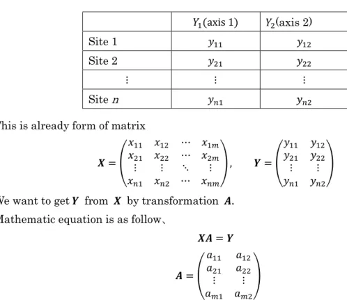
Table 46. Coordinate table of sites.
This is already form of matrix
𝑿 =
𝑥 𝑥
𝑥 𝑥
⋯ 𝑥
⋯ 𝑥
⋮ ⋮
𝑥 𝑥
⋱ ⋮
⋯ 𝑥
, 𝒀 =
𝑦 𝑦
𝑦 𝑦
⋮ 𝑦
⋮ 𝑦 We want to get 𝒀 from 𝑿 by transformation 𝑨.
Mathematic equation is as follow、
𝑿𝑨 = 𝒀
𝑨 =
𝑎 𝑎
𝑎 𝑎
⋮ 𝑎
⋮ 𝑎
The equation is question of optimization of irregular simultaneous equation.
𝑌 (axis 1) 𝑌(axis 2)
Site 1 𝑦 𝑦
Site 2 𝑦 𝑦
⋮ ⋮ ⋮
Site
n
𝑦 𝑦Theoretically, we could obtain optimum solution of 𝑨, when we knew 𝒀. However, we do not know 𝒀 actually.
When we presume that 𝒀 is expressing the points expressed by 2-dimensional coordinate such as latitude and longitude and we are requested to a table expressing distances among sites, even students in junior high school can calculate the distances using the differences using Phythagorean theorem. (This is an approximate treatment.
We cannot calculate distances on the surface of the earth without curvature of the earth.
The author is presuming approximate flatness of surface of the earth in short distance.)
Table 47. Round robin table of distances
Site 1 Site 2 ⋯ Site
n
Site1 𝑑 𝑑 ⋯ 𝑑
Site 2 𝑑 𝑑 ⋯ 𝑑
⋮ ⋮ ⋮ ⋱ ⋮
Site n
𝑑 𝑑 ⋯ 𝑑𝑑 = 0, 𝑏𝑒𝑐𝑎𝑢𝑠𝑒 𝑑 is distance between the same site, and 𝑑 = 𝑑 . Matrix expressing all distances is as follow.
𝑫 =
0 𝑑
𝑑 0
⋯ 𝑑
⋯ 𝑑
⋮ ⋮
𝑑 𝑑
⋱ ⋮
⋯ 0
Matrix 𝑫 is symmetric and diagonal matrix elements of 𝑫 is 0. Classical metric MDS is inverse operation of this calculation in which we estimate 𝒀 from given 𝑫. Some may think that is very easy procedure. They draw a line segment corresponding to the distance of a pair of sites on a flat. Then they draw a circles of which radius are corresponding to the distance to third point from an end of the line segment and draw another circle from the other end of the line segment of which radius is is the same as the other end of the line segment. The third point is existing at the inter section of the circles. Then draw three spheres from the three points on a flat in 3-dimensional space.
The 4th point is existing at the intersection of the three spheres. Repeating this we can allocate all points in (n-1)-dimensional space. This is correct. However, we have to make (n-1)-dimensional compasses for drawing distribution. There is no such a convenient tool.
I think that it is possible to draw distribution using mathematical calculation. However, if the data include measurement errors, we could not fix the points clearly and last point will have huge error range. For this reason, we cannot discuss statistical significance of the result. However, it not so bad idea to find our direction to establish adequate method. I will try this innocent idea in next paragraph.
VI-2-2-1-2. Implementation of the innocent idea. (a roundabout path)
It is not necessary to perform following operation logically. However, it is simplest example of MDS and we can learn meaning of each step of MDS.
The most famous example of Phythagorean theorem is following equation.
3 + 4 = 5 We use this as a simple example
This is right triangle. Everyone notices a method to allocate rectangle angle at origin and allocate the other angles on vertical and horizontal axes.
α(0,0), 𝛽(4, 0), 𝛾(3, 0) We express this in a matrix as follow
𝒀 = 0 0 4 0 0 3
We do not need to use our brain to find this solution. However, this is not only one solution. This is one of the possible solution. We call this solution as solution 1.
α′(−2, −1), 𝛽′(2, −1), 𝛾′(−2. 2) is another possible solution
For the confirmation, we calculate the distances
𝑑 = (2 − (−2), −1 − (−1) = (4,0) 𝑑 = (−2 − 2,2 − (−1) = (−4,3) 𝑑 = (−2 − (−2), −1 − 2) = (0, −3)
𝑑 = 4
𝑑 = (−4) + 3 = 25 = 5 𝑑 = (−3) = 3 We call this solution as solution 2.
How about next.
α′′ 1
2− √3, −1 −√3
2 , 𝛽′′ √3 +1
2, 1 −√3
2 , 𝛾′′ −√3 − 1, −1 + √3 Confirmation
𝑑 = 1
2− √3 − √3 +1
2 + −1 −√3
2 − 1 −√3
2 = 12 + 4 = 4
𝑑 = √3 +1
2− −√3 − 1 + 1 −√3
2 − −1 + √3 = 2√3 +3
2 + 2 −3√3 2
= 4 × 3 + 2 × 3√3 +9
4+ 4 − 2 × 3√3 +9 × 3
4 = 12 +9
4+ 4 +9 × 3
4 = 25 = 5
𝑑 = −√3 − 1 − 1
2− √3 + −1 + √3 − −1 −√3
2 = −3
2 + 3√3 2
=9
4+9 × 3
4 = 9 = 3
This is also one of the solutions. There are infinite number of solutions.
Solution 2: triangle α β γ′ is obtained by parallel translation of triangle αβγ by 2 to the left and by 1 to the bottom. Triangle α′′β′′γ′′ is obtained by rotating anticlockwise.
Confirmation
Matrix of rotation anticlockwise is as follow cos 𝜃 sin 𝜃
− sin 𝜃 cos 𝜃
cos𝜋
6 sin𝜋 6
− sin𝜋 6 cos𝜋
6
=
⎝
⎜
⎛
√3 2
1 2
−1 2
√3 2 ⎠
⎟
⎞
−2 −1 2 −1
−2 2
⎝
⎜
⎛
√3 2
1 2
−1 2
√3 2 ⎠
⎟
⎞=
⎝
⎜⎜
⎛ 1
2− √3 −1 −√3 2
√3 +1
2 1 −√3 2
−√3 − 1 −1 + √3⎠
⎟⎟
⎞
It is trivial that parallel translation and rotation cause no change in relative positional relationship. The implication obtained in this trial is that we can fix the shape and size of triangle from the information of distances among 3 points, though we need to consider appropriate position and angle of the viewing point by ourselves.
Question to obtain shape and size of triangle from length of three sides is typical question in elementary geometry called sine theorem and cosine theorem. Mathematically this question is essential question to obtain circumcircle of the triangle as showing in figure 79.
Fig. 79. Circumcircle of triangle Here, O is center of circumcircle, and
r
is length of radius.We assume lengths of each side as follow.
⌈AB⌉ = 𝑎, ⌈BC⌉ = 𝑏, ⌈CA⌉ = 𝑐
Point H , H , 𝑎𝑛𝑑 H are foots of perpendicular form center of the circle, and
∠OHA = ∠OHB = ∠OHC =𝜋 2
⊿OAB, ⊿OBC and ⊿OCA are isosceles triangle.
⊿OH A ≡ ⊿OH 𝑎B、⊿OH B ≡ ⊿OH C、⊿OH C ≡ ⊿OH A Most seplest proof of sine thoerem and cosine theorem is as follow At first, we make following figure
Fig.80. Sine theorem 1.
H is the foot of perpendicular from A to side BC.
⌈AH⌉ = 𝑎 sin 𝛽 = 𝑐 sin 𝛾 Concerning H’, the foot from C to side AB
𝑐 sin 𝛼 = 𝑏 sin 𝛽 Concerning H’’, the foot from B to side AC
𝑏 sin 𝛾 = 𝑎 sin 𝛼 This is sine theorem
For cosine theorem,
⌈BH⌉ = 𝑎 cos 𝛽
⌈HC⌉ = 𝑐 cos 𝛾
⌈BH⌉ + ⌈HC⌉ = ⌈BH⌉ = 𝑏
⊿AHC is rectangle triangle. Using Pythagorean theorem,
⌈AH⌉ + ⌈HC⌉ = ⌈AC⌉
𝑎 sin 𝛽 + (𝑏 − 𝑎 cos 𝛽) = 𝑐 𝑎 sin 𝛽 + 𝑏 − 2𝑎𝑏 cos 𝛽 +𝑎 cos 𝛽 = 𝑐
𝑎 sin 𝛽+𝑎 cos 𝛽 + 𝑏 − 2𝑎𝑏 cos 𝛽 = 𝑐 𝑎 (sin 𝛽 + cos 𝛽) + 𝑏 − 2𝑎𝑏 cos 𝛽 = 𝑐
𝑎 + 𝑏 − 𝑐 = 2𝑎𝑏 cos 𝛽 cos 𝛽 =𝑎 + 𝑏 − 𝑐
2𝑎𝑏 Similarly,
cos 𝛼 =𝑎 + 𝑐 − 𝑏 2𝑎𝑐 cos 𝛾 =𝑏 + 𝑐 − 𝑎
2𝑏𝑐
This is enough as a proof, though we cannot understand the relation between r and length of sides. We transform sine theorem to another form.
The relation between radius 𝑟 and angles is as follow.
Fig. 81. Sine theorem 2 We move C to C′ along the circle. At C′,
⌈BC′⌉ = 2𝑟
∠ACB and ∠AC′B are sharing the same chord AB.
∠ACB = ∠AC B = γ Line segment BC′ is diameter of the circle.
∠C AB =𝜋 2 From this,
Α
B
C’
𝑎
C 2𝑟
γ γ
𝑎
2𝑟= sin 𝛾 Similarly,
𝑏
2𝑟= sin 𝛼 𝑐
2𝑟= sin 𝛽
This is sine theorem. Following equation is mathematically more beautiful.
𝑎
sin 𝛾= 𝑏
sin 𝛼= 𝑐
sin 𝛽= 2𝑟 Frim this, we can obtain
r.
sin 𝛾 = 1 − cos 𝛾 = 1 − 𝑏 + 𝑐 − 𝑎
2𝑏𝑐 = 1
2𝑏𝑐 (4𝑏 𝑐 − (𝑏 + 𝑐 − 𝑎 ) ) (𝑏 + 𝑐 − 𝑎 ) = (𝑏 + 𝑐 ) − 2(𝑏 + 𝑐 )𝑎 + 𝑎
= 𝑏 + 2𝑏 𝑐 + 𝑐 − 2𝑎 𝑏 − 2𝑐 𝑎 + 𝑎
4𝑏 𝑐 − (𝑏 + 𝑐 − 𝑎 ) = 4𝑏 𝑐 − 𝑏 − 2𝑏 𝑐 − 𝑐 + 2𝑎 𝑏 + 2𝑐 𝑎 − 𝑎
= −𝑎 − 𝑏 − 𝑐 + 2𝑏 𝑐 + 2𝑎 𝑏 + 2𝑐 𝑎 − 𝑎
= 𝑎 𝑏 −1
2(𝑎 − 𝑏 ) + 𝑏 𝑐 −1
2(𝑏 − 𝑐 ) + 𝑐 𝑎 −1
2(𝑐 − 𝑎 )
sin 𝛾 == 1
2𝑏𝑐 𝑎 𝑏 −1
2(𝑎 − 𝑏 ) + 𝑏 𝑐 −1
2(𝑏 − 𝑐 ) + 𝑐 𝑎 −1
2(𝑐 − 𝑎 )
2𝑟 = 𝑎
sin 𝛾= 2𝑎𝑏𝑐
𝑎 𝑏 −1
2(𝑎 − 𝑏 ) + 𝑏 𝑐 −1
2(𝑏 − 𝑐 ) + 𝑐 𝑎 −1
2(𝑐 − 𝑎 )
𝑟 = 𝑎𝑏𝑐
𝑎 𝑏 −1
2(𝑎 − 𝑏 ) + 𝑏 𝑐 −1
2(𝑏 − 𝑐 ) + 𝑐 𝑎 −1
2(𝑐 − 𝑎 )
Using sine theorem and cosine theorem, we could obtain shape and size of triangle. The size can be expressed by 𝑟 of circumcircle.
Let us go back to first figure of circumcircle (Fig.79). Central angle ∠AOB is sharing the same chord AB with angle of circumference ∠ACB. Central angle is twice of circumference angle. Therefor,
∠AOB = 2γ Similarly,
∠BOC = 2α
∠COA = 2𝛽 We have to decide the rotation of the triangle.
The author thinks that easiest calculation is the best. We allocate vector OA⃗ on horizontal axis. VectorOB⃗ is obtained by rotating vector OA⃗ 2γ anticlockwise, and vector OC⃗ is obtained by rotating vector OA⃗ 2𝛽 clockwise.
Formula of rotation anticlockwise is following matrix.
cos 𝜃 sin 𝜃
− sin 𝜃 cos 𝜃 Conclusively,
OB = (𝑟 0) cos 2𝛾 sin 2𝛾
− sin 2𝛾 cos 2𝛾 OB = (𝑟 0) cos 2𝛾 sin 2𝛾
− sin 2𝛾 cos 2𝛾
= (𝑟cos 2𝛾 𝑟 sin 2𝛾) = (𝑟(1 − 2 sin 𝛾) 2𝑟 sin 𝛾 cos 𝛾)
= 𝑟(1 − 2 𝑎
2 ) 2𝑟 𝑎 2
𝑏 + 𝑐 − 𝑎 2𝑏𝑐
= 𝑟(1 −𝑎
2 ) 𝑟𝑎 𝑏 + 𝑐 − 𝑎 2𝑏𝑐 OC = (𝑟 0) cos −2𝛽 sin −2𝛽
− sin −2𝛽 cos −2𝛽 = (𝑟 0) cos 2𝛽 − sin 2𝛽
sin 2𝛽 cos 2𝛽 = (𝑟cos 2𝛽 − rsin 2𝛽)
= 𝑟(1 −𝑐
2 ) 𝑟𝑎 𝑏 + 𝑎 − 𝑐 2𝑎𝑏
The author does this calculation for the first time in 50yeas after graduation of junior high school. We cannot expand this method to higher dimensional space directly. For this reason, we can say that we did meaningless trial. However, when we can make triangle as a flat, we can make multi-dimensional polyhedron in multi-dimensional space by connecting triangle. Following is an example of 4 points in 3-dimensional space.
Fig.82. Cubic diagram of 4 points and origin.
When distances between A and B, A and C, A and D, B and C, B and D and D and C are
given correctly, we can make tetrahedron. When we fix the origin of the coordinate, we can express the distance as follow.
AB = ⌈𝑉 − 𝑉 ⌉ AC = ⌈𝑉 − 𝑉 ⌉ AD = ⌈𝑉 − 𝑉 ⌉ BC = ⌈𝑉 − 𝑉 ⌉ BD = ⌈𝑉 − 𝑉 ⌉ CD = ⌈𝑉 − 𝑉 ⌉
This relation is stable when we move the origin of vectors to the other points as shown in figure 82. In the case there are more than 5 points, if all distances are measured correctly and they have only 3-dimensional elements. We can make more complex polyhedron in 3-dimensional space. As shown in the figure 82, we can allocate the origin of the space in any point in the space.
VI-2-2-1-3. Classical MDS (Metric MDS) Given data is following distance matrix.
𝑫 =
0 𝐷
𝐷 0
⋯ 𝐷
⋯ ⋯ ⋯ 𝐷
𝐷 𝐷 ⋱ ⋮
⋯ 0 We define matrix of square of distances as follow.
𝑫𝟐=
0 𝐷
𝐷 0
⋯ 𝐷
⋯ ⋯ ⋯ 𝐷
𝐷 𝐷 ⋱ ⋮
⋯ 0
In this chapter, 𝑫𝟐 is not square of 𝑫.
We want to know the vectors from origin to each point. The matrix of vector is as follow.
𝑽 = 𝑽 𝑽
⋮ 𝑽𝒏
𝐷 = 𝑽 − 𝑽 When the Vectors have
m
-dimension𝑽 =
𝑣 𝑣 ⋯ 𝑣
𝑣 𝑣 ⋯ 𝑣
⋮ ⋮ ⋱ ⋮
𝑣 𝑣 ⋯ 𝑣
From trial of our innocent idea, we could make clear the procedure of calculation of MDS, and we understood that we have to allocate origin of coordinate by ourselves considering visual effects. This is essential, as coordinate and viewing direction are strongly affect
our recognition of phenomena. Most general idea is allocating coordinate on the median point of the data. Median point is representative of all data. When we select origine of coordinate on median point of the data, that means we treat all data in even weight. This makes easier the calculation statistical calculations.
Grabbing vertex of triangle formed by two vectors at origin putting the distance on the base of triangle. Making tetrahedron from 3 triangles. Lining the tetrahedrons in all the direction of the space. This procedure is analogical image of MDS. For this, we use centralization matrix. Generally, we use parallel translation for this procedure. We can express the procedure in a formula by using centralization matrix.
It is too hastily to show the formula. The author explains the function of centralization matrix step by step from single parallel translation.
Translation of coordination to median point is subtraction of average coordinate from each coordinate datum. This is expressed as follow.
𝑣 −1
𝑛 𝑣
Second term of the equation means average (median point).
When we expand sign of sum, it expressed as follow.
𝑣 −1
𝑛𝑣 −1
𝑛𝑣 − ⋯1 𝑛𝑣 Then we transform this as follow
−1
𝑛𝑣 −1
𝑛𝑣 − ⋯ + 1 −1
𝑛 𝑣 − ⋯ −1 𝑛𝑣 This can be expressed by following inner product of two vectors.
−1
𝑛𝑣 −1
𝑛𝑣 − ⋯ + 1 −1
𝑛 𝑣 − ⋯ −1
𝑛𝑣 = −1 𝑛 −1
𝑛 ⋯ 1 −1 𝑛⋯ −1
𝑛
⎝
⎜⎜
⎛ 𝑣 𝑣 𝑣⋮
⋮ 𝑣 ⎠
⎟⎟
⎞
We can expressed all translation by following multiplication of matrixes.
𝑽 =
𝑣 𝑣 ⋯ 𝑣
𝑣 𝑣 ⋯ 𝑣
⋮ ⋮ ⋱ ⋮
𝑣 𝑣 ⋯ 𝑣
𝑽 =
⎝
⎜
⎜
⎜
⎛ 1 −1
𝑛 −1
𝑛 ⋯ −1 𝑛
−1
𝑛 1 −1
𝑛 ⋯ −1
⋮ ⋮ ⋱ ⋮ 𝑛
−1 𝑛 −1
𝑛 ⋯ 1 −1 𝑛⎠
⎟
⎟
⎟
⎞ 𝑣 𝑣 ⋯ 𝑣
𝑣 𝑣 ⋯ 𝑣
⋮ ⋮ ⋱ ⋮
𝑣 𝑣 ⋯ 𝑣
We call following matrix as centralizing matrix.
𝑮 =
⎝
⎜
⎜
⎜
⎛ 1 −1
𝑛 −1
𝑛 ⋯ −1 𝑛
−1
𝑛 1 −1
𝑛 ⋯ −1
⋮ ⋮ ⋱ ⋮ 𝑛
−1 𝑛 −1
𝑛 ⋯ 1 −1 𝑛⎠
⎟
⎟
⎟
⎞
Formula 76 General expression of the matrix is as follow
𝑮 = 𝑰 −1 𝑛𝟏𝒏𝟏 𝑰 is 𝑛 × nunit vector.
𝟏𝒏= 1 1⋮ 1
𝟏𝒏 = (1 1 ⋯ 1) From this,
𝟏𝒏𝟏 = 1 1 1 1
⋯ 1
⋮ ⋮ ⋯ 1 1 1
⋱ ⋮
⋯ 1
𝟏𝒏𝟏 𝟐= 𝑛 𝑛 𝑛 𝑛
⋯ 𝑛
⋯ 𝑛
⋮ ⋮ 𝑛 𝑛
⋱ ⋮
⋯ 𝑛
= 𝑛 1 1 1 1
⋯ 1
⋮ ⋮ ⋯ 1 1 1
⋱ ⋮
⋯ 1
= 𝑛𝟏𝒏𝟏 Centralizing matrix 𝑮 has unique and convenient characteristics.
First,
𝑮 𝒌= 𝑮 Confirmation
𝑮 𝟐= 𝑰 −1
𝑛𝟏𝒏𝟏 𝑰 −1 𝑛𝟏𝒏𝟏
= 𝑰 𝑰 − 𝟐𝑰 1
𝑛𝟏𝒏𝟏 + 1
𝑛 𝟏𝒏𝟏 𝟐
= 𝑰 −1
𝑛𝟏𝒏𝟏 = 𝑮
∵ 𝑰 𝑰 = 𝑰 , 𝑰 𝟏𝒏𝟏 = 𝟏𝒏𝟏 , 𝟏𝒏𝟏 𝟐= 𝑛𝟏𝒏𝟏
This is logically trivial. Because, center is only one. When we centralize data, we cannot centralize any more. However, this character is important in the calculation. As an
example, we centralize 𝐀 = 𝑎 𝑏𝑐 𝑑
by 𝑮 .
This is the inverse operation of the operation in which we make centralizing matrix.
𝑮 𝑨 = 𝑰 −1 4𝟏𝟒𝟏
𝑎 𝑏𝑐 𝑑
= 1 0 0 1
0 0 0 0 0 0 0 0
1 0 0 1
𝑎 𝑏𝑐 𝑑
−1 4
1 1 1 1
1 1 1 1 1 1 1 1
1 1 1 1
𝑎 𝑏𝑐 𝑑
= 𝑎 𝑏𝑐 𝑑
−1 4
𝑎 + 𝑏 + 𝑐 + 𝑑 𝑎 + 𝑏 + 𝑐 + 𝑑 𝑎 + 𝑏 + 𝑐 + 𝑑 𝑎 + 𝑏 + 𝑐 + 𝑑
=
⎝
⎜⎜
⎜⎜
⎜
⎛
𝑎 −𝑎 + 𝑏 + 𝑐 + 𝑑 4 𝑏 −𝑎 + 𝑏 + 𝑐 + 𝑑
4 𝑐 −𝑎 + 𝑏 + 𝑐 + 𝑑
4 𝑑 −𝑎 + 𝑏 + 𝑐 + 𝑑
4 ⎠
⎟⎟
⎟⎟
⎟
⎞
Second term in each factor is written by fraction. The fraction means average.
𝑮 (𝑮 𝑨) = 1 0 0 1
0 0 0 0 0 0 0 0
1 0 0 1
⎝
⎜⎜
⎜⎜
⎜
⎛
𝑎 −𝑎 + 𝑏 + 𝑐 + 𝑑 4 𝑏 −𝑎 + 𝑏 + 𝑐 + 𝑑
4 𝑐 −𝑎 + 𝑏 + 𝑐 + 𝑑
4 𝑑 −𝑎 + 𝑏 + 𝑐 + 𝑑
4 ⎠
⎟⎟
⎟⎟
⎟
⎞
−1 4
1 1 1 1
1 1 1 1 1 1 1 1
1 1 1 1
⎝
⎜⎜
⎜⎜
⎜
⎛
𝑎 −𝑎 + 𝑏 + 𝑐 + 𝑑 4 𝑏 −𝑎 + 𝑏 + 𝑐 + 𝑑
4 𝑐 −𝑎 + 𝑏 + 𝑐 + 𝑑
4 𝑑 −𝑎 + 𝑏 + 𝑐 + 𝑑
4 ⎠
⎟⎟
⎟⎟
⎟
⎞
=
⎝
⎜⎜
⎜⎜
⎜
⎛
𝑎 −𝑎 + 𝑏 + 𝑐 + 𝑑 4 𝑏 −𝑎 + 𝑏 + 𝑐 + 𝑑
4 𝑐 −𝑎 + 𝑏 + 𝑐 + 𝑑
4 𝑑 −𝑎 + 𝑏 + 𝑐 + 𝑑
4 ⎠
⎟⎟
⎟⎟
⎟
⎞
−1 4
𝑎 + 𝑏 + 𝑐 + 𝑑 − (𝑎 + 𝑏 + 𝑐 + 𝑑) 𝑎 + 𝑏 + 𝑐 + 𝑑 − (𝑎 + 𝑏 + 𝑐 + 𝑑) 𝑎 + 𝑏 + 𝑐 + 𝑑 − (𝑎 + 𝑏 + 𝑐 + 𝑑) 𝑎 + 𝑏 + 𝑐 + 𝑑 − (𝑎 + 𝑏 + 𝑐 + 𝑑)
=
⎝
⎜⎜
⎜⎜
⎜
⎛
𝑎 −𝑎 + 𝑏 + 𝑐 + 𝑑 4 𝑏 −𝑎 + 𝑏 + 𝑐 + 𝑑
4 𝑐 −𝑎 + 𝑏 + 𝑐 + 𝑑
4 𝑑 −𝑎 + 𝑏 + 𝑐 + 𝑑
4 ⎠
⎟⎟
⎟⎟
⎟
⎞
− 0 =
⎝
⎜⎜
⎜⎜
⎜
⎛
𝑎 −𝑎 + 𝑏 + 𝑐 + 𝑑 4 𝑏 −𝑎 + 𝑏 + 𝑐 + 𝑑
4 𝑐 −𝑎 + 𝑏 + 𝑐 + 𝑑
4 𝑑 −𝑎 + 𝑏 + 𝑐 + 𝑑
4 ⎠
⎟⎟
⎟⎟
⎟
⎞
= 𝑮 𝑨
We confirmed
𝑮 (𝑮 𝑨) = (𝑮 𝑮 ) 𝑨 = 𝑮 𝑨 Secondly, 𝑮 has following character.
𝑮 𝟏𝒏= 𝟏𝒏 𝑮 = 0 Confirmation
𝑮 𝟏𝒏= 𝑰 −1
𝑛𝟏𝒏𝟏 𝟏𝒏= 𝑰 𝟏𝒏−1
𝑛𝟏𝒏 𝟏 𝟏𝒏 = 𝟏𝒏−1
𝑛𝑛𝟏𝒏= 0 𝑮 𝟏𝒏= 𝟏𝒏 𝑰 −1
𝑛𝟏𝒏𝟏 = 𝟏𝒏 𝑰 −1
𝑛 𝟏𝒏 𝟏𝒏 𝟏 = 𝟏𝒏 −1
𝑛𝑛𝟏𝒏 = 0
We go back to matrix 𝑽.
This is a matrixed obtained by lining up row vectors vertically as follow.
𝑽 = 𝑽 𝑽
⋮ 𝑽𝒏
=
𝑣 𝑣 ⋯ 𝑣
𝑣 𝑣 ⋯ 𝑣
⋮ ⋮ ⋱ ⋮
𝑣 𝑣 ⋯ 𝑣
We consider matrix 𝑽𝑽 .
The author calls the matrix “matrix of inner products” personally. Because we call 𝑽 𝑽 of which factors are composed from variance and covariance of elements of data as variance-covariance matrix, and factors of 𝑽𝑽 are inner products of vector. Actually, this naming is not used generally. This naming may make confusion because matrix is a kind of vector, because we can consider inner product between matrixes, 𝑽 ∙ 𝑽 . We call this inner product of matrix. Inner product of matrix is a scalar and name of inner product of matrix is authorized. It is better not to use “matrix of inner products” in other places in order prevent confusion. However, we call 𝑽𝑽 as “matrix of inner products”
here. It is important to confirm 𝑽𝑽 ≠ 𝑽 ∙ 𝑽
𝑽𝑽 = 𝑽𝟏
𝑽𝟐
⋮ 𝑽𝒏
(𝑽𝟏 𝑽𝟐 ⋯ 𝑽𝒏) =
⎝
⎜
⎛
𝑽𝟏∙ 𝑽𝟏 𝑽𝟏∙ 𝑽𝟐 𝑽𝟐∙ 𝑽𝟏 𝑽𝟐∙ 𝑽𝟐
⋯ 𝑽𝟏∙ 𝑽𝒏
⋯ 𝑽𝟐∙ 𝑽𝒏
⋮ ⋮
𝑽𝒏𝑽𝟏 𝑽𝒏𝑽𝟐
⋱ ⋮
⋯ 𝑽𝒏𝑽𝒏 ⎠
⎟
⎞
𝑽𝒊∙ 𝑽𝒋 is inner product of vector 𝑽𝒊 and 𝑽𝒋
𝑽𝒊∙ 𝑽𝒋 = (𝑣 ⋯ 𝑣 ) 𝑣
⋮ 𝑣
Then we consider matrix of inner product of centralized matrix.
𝑽 = 𝑮𝒎𝑽
From cosine theorem, we can express the relation among vectors as follow.
𝟐𝑽′ ∙ 𝑽′ = ⌈𝑽′ ⌉𝟐+ 𝑽′ 𝟐− 𝑽′ − 𝑽′ 𝟐
The last term of the right side is square of distance between arrow heads of both vectors.
𝑽′ − 𝑽′ 𝟐= 𝑑 𝟐𝑽′ ∙ 𝑽′ = ⌈𝑽′ ⌉𝟐+ 𝑽′ 𝟐− 𝑑
This is relation in each factor of matrix. We express this in the form of matrix.
𝟐𝑽 𝑽𝑻= 𝟏𝑛𝟏𝑛 𝑑𝑖𝑎𝑔(𝑽 𝑽𝑻) + 𝑑𝑖𝑎𝑔𝑽 𝑽 𝟏𝑛𝟏𝑛 − 𝑫𝟐 In this, 𝑑𝑖𝑎𝑔
A
ismatrix composed only from diagonal factor of matrixA.
Expansion of this calculation is as follow.
𝟐𝑽 𝑽𝑻=
1 1 ⋯ 1 1 1 ⋯ 1
⋮ 1
⋮ 1
⋱
⋯
⋮ 1 ⎝
⎜
⎛
𝑽′ 0 ⋯ 0
0 𝑽′ ⋯ 0
⋮ 0
⋮ 0
⋱
⋯
⋮ 𝑽′ ⎠
⎟
⎞+
⎝
⎜
⎛
𝑽′ 0 ⋯ 0
0 𝑽′ ⋯ 0
⋮ 0
⋮ 0
⋱
⋯
⋮ 𝑽′ ⎠
⎟
⎞ 1 1 ⋯ 1 1 1 ⋯ 1
⋮ 1
⋮ 1
⋱
⋯
⋮ 1
− 𝑫𝟐
We transform left side by
𝑽 𝑽𝑻= 𝑮𝒏𝑽(𝑮𝒏𝑽)𝑻= 𝑮𝒏𝑽𝑽 𝑮𝒏 = 𝑮𝒏𝑽𝑽 𝑮𝒏
𝟐𝑮𝒏𝑽𝑽 𝑮𝒏=
⎝
⎜
⎛
𝑽′ 𝑽′ ⋯ 𝑽′
𝑽′ 𝑽′ ⋯ 𝑽′
⋮ 𝑽′
⋮ 𝑽′
⋱
⋯
⋮ 𝑽′ ⎠
⎟
⎞+
⎝
⎜
⎛
𝑽′ 𝑽′ ⋯ 𝑽′
𝑽′ 𝑽′ ⋯ 𝑽′
⋮ 𝑽′
⋮ 𝑽′
⋱
⋯
⋮ 𝑽′ ⎠
⎟
⎞− 𝑫𝟐
We multiply 𝑮𝒏 from left and right to both sides.
𝟐𝑮𝒏 𝑽𝑽 𝑮𝒏 = 𝑮𝒏
⎝
⎜
⎛
𝑽′ 𝑽′ ⋯ 𝑽′
𝑽′ 𝑽′ ⋯ 𝑽′
⋮ 𝑽′
⋮ 𝑽′
⋱
⋯
⋮ 𝑽′ ⎠
⎟
⎞𝑮𝒏+ 𝑮𝒏
⎝
⎜
⎛
𝑽′ 𝑽′ ⋯ 𝑽′
𝑽′ 𝑽′ ⋯ 𝑽′
⋮ 𝑽′
⋮ 𝑽′
⋱
⋯
⋮ 𝑽′ ⎠
⎟
⎞𝑮𝒏− 𝑮𝒏𝑫𝟐𝑮𝒏
From the characteristic of Centralizing matrix.
𝑮𝒏 = 𝑮𝒏
Left size is
𝑮𝒏 𝑽𝑽 𝑮𝒏 = 𝑮𝒏𝑽𝑽 𝑮𝒏
Concerning right side, first and second term are 0. Confirmation is as follow.
𝑮𝒏
𝑽′12 𝑽′22 ⋯ 𝑽′𝑛2 𝑽′12 𝑽′22 ⋯ 𝑽′𝑛2
⋮ 𝑽′12
⋮ 𝑽′22
⋱
⋯
⋮ 𝑽′𝑛2
When we focus on first column of second vector. First column is lining up of square of the same vector as follow. This means that first row of first column of obtainable matrix is as follow.
𝑮𝒏
⎝
⎜
⎛ 𝑽′
𝑽′
⋮ 𝑽′ ⎠
⎟
⎞= 𝑽′ 𝑮𝒏 1 1⋮ 1
= 0
∵ 𝑮𝒏 1 1⋮ 1
= 0 from character of centralizing matrix Similarly, all the other factors in obtainable matrix are 0. Consequently,
𝑮𝒏
𝑽′12 𝑽′22 ⋯ 𝑽′𝑛2 𝑽′12 𝑽′22 ⋯ 𝑽′𝑛2
⋮ 𝑽′12
⋮ 𝑽′22
⋱
⋯
⋮ 𝑽′𝑛2
= 0
Similarly, concerning second term,
⎝
⎜
⎛
𝑽′ 𝑽′ ⋯ 𝑽′
𝑽′ 𝑽′ ⋯ 𝑽′
⋮ 𝑽′
⋮ 𝑽′
⋱
⋯
⋮ 𝑽′ ⎠
⎟
⎞𝑮𝒏
First row of obtainable matrix is as follow
𝑽 𝑽 ⋯ 𝑽 𝑮𝒏= 𝑽 (1 1 ⋯ 1)𝑮𝒏= 0 Similarly, other factors in obtainable matrix is 0, and
⎝
⎜
⎛
𝑽′ 𝑽′ ⋯ 𝑽′
𝑽′ 𝑽′ ⋯ 𝑽′
⋮ 𝑽′
⋮ 𝑽′
⋱
⋯
⋮ 𝑽′ ⎠
⎟
⎞𝑮𝒏= 0
Conclusively,
𝟐𝑮𝒏𝑽𝑽 𝑮𝒏= −𝑮𝒏𝑫𝟐𝑮𝒏
By this transformation, right side distances matrix can be explained by “matrix of inner products”.
We can give position in a space to 𝑫𝟐 which was roving in inanity by folding 𝑮𝒏. The author can give safe refuge to Hebrews. The author is brushing brisk breeze doing good.
We want to know𝑮𝒏𝑽
𝒀 = 𝑮𝒏𝑽
𝒀 = (𝑮𝒏𝑽) = 𝑽 𝑮𝒏 𝒀𝒀 = 𝑮𝒏𝑽𝑽 𝑮𝒏 =−1
2𝑮𝒏𝑫𝟐𝑮𝒏 At first, we calculate,
𝒁 = −1
2𝑮𝒏𝑫𝟐𝑮𝒏 Then we do spectral decomposition of 𝒁
𝒁 = 𝑷𝚲𝑷 𝟏= 𝑷𝚲𝟏𝟐𝚲𝟏𝟐𝑷 𝟏= 𝑷𝚲𝟏𝟐𝚲𝟏𝟐𝑷 = 𝑷𝚲𝟏𝟐 𝑷𝚲𝟏𝟐
−1
2𝑮𝒏𝑫𝟐𝑮𝒏=𝑷𝚲𝟏𝟐 𝑷𝚲𝟏𝟐
T
Then
𝒀 = 𝑷𝚲𝟏𝟐
Formula 77 VI-2-2-2. Theoretical discussions about classical MDS
There is a data
X
which obtained by observation. Each datum ofX
is composed fromm
elements. X is expressed by 𝑛 data which has 𝑚 elements as following matrix.𝑿 =
𝑥 𝑥 𝑥 𝑥
⋯ 𝑥
⋯ 𝑥
⋮ ⋮
𝑥 𝑥
⋱ ⋮
⋯ 𝑥
It is difficult to understand structure of distribution of all data and relationship among data, when a lot of elements is existing. We want to summarize the data combining several elements to reduce the number of elements from 𝑚 to 𝑙 (𝑙 < 𝑚). This is motivation of MDS and PCA. Most extreme case we want reduce the number to only one (𝑙 = 1).
y = 𝑎 𝑥 + 𝑎 𝑥 + ⋯ + 𝑎 𝑥 As matrix calculation
𝒀 = 𝑿𝑨
𝑨 = (𝑎 𝑎 ⋯ 𝑎 ) In the case 𝑙 > 1,
𝑨 = 𝑎
⋮ 𝑎
𝑎
⋮
𝑎 ⋯
𝑎
⋮ 𝑎
𝒀 = 𝑿𝑨 =
𝑦 ⋯ 𝑦
⋮ ⋱ ⋮
𝑦 ⋯ 𝑦
When number of data(𝑛)is larger than number of elements (𝑝), the simultaneous equation is irregular, and data include error generally. For this reason, we optimize 𝑨 by minimizing differences between observed data and expected values.
𝒀 − 𝒀
𝒀 − 𝒀 is norm expressing the magnitude of difference between two vectors. We consider Euclidian norm in orthogonal space.
𝒀 − 𝒀 = 𝒀 − 𝒀
In the MDS which express the data in plotting data in 2-dimensinal flat is summarizing the all elements to two representative elements. In this meaning, MDS is a kind of approximation by least square method. However, the data are given as form of the difference of among elements. Thus, we have to make “matrix of inner products after centralization of the given data as follow.
𝒁 = −1
2𝑮𝒏𝑫𝟐𝑮𝒏
Then, we implement diagonalization of this matrix in order to make form of 𝑷𝜦𝟏𝟐𝜦𝟏𝟐𝑷 .。
𝑷𝜦𝟏𝟐𝜦𝟏𝟐𝑷 = 𝑷𝜦𝟏𝟐 𝑷𝜦𝟏𝟐
Right side is form of “matrix of inner products” 𝑿𝑿 , when we consider 𝑿 = 𝑷𝜦𝟏𝟐
In singular value decomposition, we made variance-covariance matrix 𝑿 𝑿 and “matrix of inner products” 𝑿𝑿 , and then we diagonalize both matrixes.
𝑿𝑿 = 𝑷𝜦𝑷 𝑿 𝑿 = 𝑸𝜦𝑸 𝑷 = 𝑼 𝑸 = 𝑽 𝑿 = 𝑼𝜮𝑽 = 𝑼𝜦 𝜦 𝑽
In MDS, we are not given vector data which has direction. We cannot make variance - covariance matrix and matrix of inner products directly.
However, we can give direction to the data by centralization, and we can diagonalize 𝑮𝒏𝑫𝟐𝑮𝒏 considering 𝑿 =𝑮𝒏𝑫
𝑿𝑿 = 𝑷𝜦𝑷
When we consider that “matrix of inner products” is reverse of variance-covariance matrix, we can say that MDS is reverse of PCA. We are expecting that components which have higher contribution rate are concentrated in 2 or 3 directions in PCA and MDS and make 2-dimensional plot or 3-dimensional plot. Most interesting function of MDS is plotting data of which dimension we do not know on 2 or 3dimensional space. However, components do not always concentrate to seldom direction. Analyzers who know that MDS is selecting several representative axes from orthogonal axes can understand importance of confirmation of cumulative contribution ratio in analysis. The author personally interested in drawing plotts using miner importance axis. We may discover new findings from minor relation. PCA and MDS are methods to see phenomena from various viewing points. Knowing mathematical meaning of MDS, you can use this tool for unique and interesting findings.
VI-2-2-3. Several examples of calculation of MDS.
The author perform calculation of MDS of simple examples in this paragraph aiming deepening the calculation and meaning of MDS and PCA.
Example 1 (equilateral triangle)
We allocate of vertexes of equilateral triangle which length of sides is 1 in a space. It is easy to understand direction of viewing point, because, three points make triangle on a flat naturally. We confirm whether the triangle can be drawn on 2-dimensional flat from the information of distances among vertexes.
Round robin square of distance matrix is as follow 𝑫𝟐=
0 1 1 1 0 1 1 1 0 Centralization
𝑮𝒏𝑫 𝑮𝒏 =
⎝
⎜⎜
⎛ 1 −1
3 −1
3 −1 3
−1
3 1 −1 3 −1
3
−1
3 −1
3 1 −1 3⎠
⎟⎟
⎞ 0 1 1 1 0 1 1 1 0
⎝
⎜⎜
⎛ 1 −1
3 −1
3 −1 3
−1
3 1 −1 3 −1
3
−1
3 −1
3 1 −1 3⎠
⎟⎟
⎞
⎝
⎜⎜
⎛ 2 3 −1
3 −1 3
−1 3
2 3 −1
3
−1 3 −1
3 2 3 ⎠
⎟⎟
⎞ 0 1 1 1 0 1 1 1 0
⎝
⎜⎜
⎛ 2 3 −1
3 −1 3
−1 3
2 3 −1
3
−1 3 −1
3 2 3 ⎠
⎟⎟
⎞
⎝
⎜⎜
⎛
−2 3
1 3
1 1 3
3 −2 3
1 1 3
3 1 3 −2
3⎠
⎟⎟
⎞
⎝
⎜⎜
⎛ 2 3 −1
3 −1 3
−1 3
2 3 −1
3
−1 3 −1
3 2 3 ⎠
⎟⎟
⎞
⎝
⎜⎜
⎛
−6 9
3 9
3 3 9
9 −6 9
3 3 9
9 3 9 −6
9⎠
⎟⎟
⎞
=1 3
−2 1 1 1 −2 1 1 1 −2
We diagonalize −2 1 1 1 −2 1 1 1 −2
.
We solve eigen equation to obtain eigenvalue.
。
−2 − 𝜆 1 1
1 −2 − 𝜆 1
1 1 −2 − 𝜆
= 0
−(2 + 𝜆) + 2 + 3(2 + 𝜆)
−(𝜆 + 4𝜆 + 4)(2 + 𝜆) + 2 + 3(2 + 𝜆)
−𝜆 − 4𝜆 − 4𝜆 − 2𝜆 − 8𝜆 − 8 + 2 + 6 + 3𝜆
−𝜆 − 6𝜆 − 12𝜆 − 8 + 2 + 6 + 3𝜆 = 0
−𝜆 − 6𝜆 − 9𝜆 = 0 𝜆(𝜆 + 3) = 0 𝜆 = 0, 𝜆 = −3 We calculate eigenvector belonging to 𝜆 = 0.
2 −1 −1
−1 2 −1
−1 −1 2 𝑥 𝑥 𝑥 = 0
𝑥 𝑥 𝑥 2𝑥 − 𝑥 − 𝑥 = 0
−𝑥 + 2𝑥 − 𝑥 = 0
−𝑥 −𝑥 + 2𝑥 = 0 From all equation we obtain
𝑥 = 𝑥 = 𝑥 We select following vector as most simple eigen vector.
1 1 1
Then we calculate eigenvector belonging to 𝜆 = −3.
2 −1 −1
−1 2 −1
−1 −1 2 𝑥 𝑥
𝑥 = −3𝜆 = 0
−2𝑥 + 𝑥 + 𝑥 = −3𝑥 𝑥 − 2𝑥 + 𝑥 = −3𝑥 𝑥 + 𝑥 − 3𝑥 = −3𝑥 From all equation
𝑥 + 𝑥 + 𝑥 = 0 We select following equation.
2
−1
−1
We make the other eigen vector belonging to 𝜆 = −3 using orthogonality. The vector should be orthogonal to two vectors obtained in upper calculation.
(𝑥 𝑥 𝑥 ) 1 1 1
= 0
(𝑥 𝑥 𝑥 ) 2
−1
−1
= 0 𝑥 + 𝑥 + 𝑥 = 0 2𝑥 − 𝑥 − 𝑥 = 0 We solve this simultaneous equation and obtain
𝑥 = 0, 𝑥 = −𝑥 We select following vector as simplest eigenvector.
0 1
−1
From upper equation we could obtain diagonalizing matrix of −2 1 1 1 −2 1 1 1 −2
as follow.
𝑷 =
−2 0 1
1 1 1
1 −1 1
It is not necessary, though the author transform this to unit vector for future convenience.
𝑷 =
⎝
⎜⎜
⎜
⎛
√2
√3 0 1
√3
− 1
√6 1
√2 1
√3
− 1
√6 − 1
√2 1
√3⎠
⎟⎟
⎟
⎞
𝑷 is diagonalization matrix of symmetric matrix. Consequently, 𝑷 𝟏= 𝑷
𝜦 =
𝜆 0 0 𝜆
… 0
… 0
⋮ ⋮ 0 0
⋱ ⋮
… 𝜆
=
−3 0 0 0 −3 0
0 0 0
|𝜆 | ≥ |𝜆 | ≥ ⋯ ≥ |𝜆 | Using these matrixes, we can diagonalize 𝑮𝒏𝑫 𝑮𝒏 as follow.
𝑮𝒏𝑫 𝑮𝒏 = 𝑷𝜦𝑷
1 3
−2 1 1 1 −2 1 1 1 −2
=1 3
⎝
⎜⎜
⎜
⎛
√2
√3 0 1
√3
− 1
√6 1
√2 1
√3
− 1
√6 − 1
√2 1
√3⎠
⎟⎟
⎟
⎞ −3 0 0 0 −3 0
0 0 0
⎝
⎜⎜
⎜
⎛
√2
√3 − 1
√6 − 1
√6
0 1
√2 − 1
√2 1
√3 1
√3 1
√3 ⎠
⎟⎟
⎟
⎞
=1 3
⎝
⎜⎜
⎜
⎛
√2
√3 0 1
√3
− 1
√6 1
√2 1
√3
− 1
√6 − 1
√2 1
√3⎠
⎟⎟
⎟
⎞ −3 0 0 0 −3 0
0 0 0
⎝
⎜⎜
⎜
⎛
√2
√3 − 1
√6 − 1
√6
0 1
√2 − 1
√2 1
√3 1
√3 1
√3 ⎠
⎟⎟
⎟
⎞
⎝
⎜⎜
⎜
⎛
√2
√3 0 1
√3
− 1
√6 1
√2 1
√3
− 1
√6 − 1
√2 1
√3⎠
⎟⎟
⎟
⎞ −1 0 0 0 −1 0
0 0 0
⎝
⎜⎜
⎜
⎛
√2
√3 − 1
√6 − 1
√6
0 1
√2 − 1
√2 1
√3 1
√3 1
√3 ⎠
⎟⎟
⎟
⎞
𝒁 =𝑮𝒏𝑫 𝑮𝒏
−𝟐
= 1
−2
⎝
⎜⎜
⎜
⎛
√2
√3 0 1
√3
− 1
√6 1
√2 1
√3
− 1
√6 − 1
√2 1
√3⎠
⎟⎟
⎟
⎞ −1 0 0 0 −1 0
0 0 0
⎝
⎜⎜
⎜
⎛
√2
√3 − 1
√6 − 1
√6
0 1
√2 − 1
√2 1
√3 1
√3 1
√3 ⎠
⎟⎟
⎟
⎞
=
⎝
⎜⎜
⎜
⎛
√2
√3 0 1
√3
− 1
√6 1
√2 1
√3
− 1
√6 − 1
√2 1
√3⎠
⎟⎟
⎟
⎞
⎝
⎜
⎛ 1 2 0 0 0 1
2 0 0 0 0⎠
⎟
⎞
⎝
⎜⎜
⎜
⎛
√2
√3 − 1
√6 − 1
√6
0 1
√2 − 1
√2 1
√3 1
√3 1
√3 ⎠
⎟⎟
⎟
⎞
We transform this to the form of𝑷𝜦𝟏𝟐𝜦𝟏𝟐𝑷 .
𝑷𝜦𝟏𝟐𝜦𝟏𝟐𝑷 =
⎝
⎜⎜
⎜
⎛
√2
√3 0 1
√3
− 1
√6 1
√2 1
√3
− 1
√6 − 1
√2 1
√3⎠
⎟⎟
⎟
⎞
⎝
⎜
⎛ 1
√2 0 0 0 1
√2 0 0 0 0⎠
⎟
⎞
⎝
⎜
⎛ 1
√2 0 0 0 1
√2 0 0 0 0⎠
⎟
⎞
⎝
⎜⎜
⎜
⎛
√2
√3 − 1
√6 − 1
√6
0 1
√2 − 1
√2 1
√3 1
√3 1
√3 ⎠
⎟⎟
⎟
⎞
This is result means eigenvector
⎝
⎜
⎛√
√
√ ⎠
⎟
⎞ has no expansion to its direction. We can neglect
this axis.
𝑷𝜦𝟏𝟐𝜦𝟏𝟐𝑷 =
⎝
⎜⎜
⎜
⎛
√2
√3 0
− 1
√6 1
√2
− 1
√6 − 1
√2⎠
⎟⎟
⎟
⎞
⎝
⎜
⎛ 1
√2 0 0 1
√2⎠
⎟
⎞
⎝
⎜
⎛ 1
√2 0 0 1
√2⎠
⎟
⎞
⎝
⎜
⎛
√2
√3 − 1
√6 − 1
√6
0 1
√2 − 1
√2⎠
⎟
⎞
𝑷𝜦𝟏𝟐=
⎝
⎜⎜
⎜
⎛
√2
√3 0
− 1
√6 1
√2
− 1
√6 − 1
√2⎠
⎟⎟
⎟
⎞
⎝
⎜
⎛ 1
√2 0 0 1
√2⎠
⎟
⎞=
⎝
⎜⎜
⎜
⎛ 1
√3 0
− 1 2√3
1 2
− 1 2√3 −1
2⎠
⎟⎟
⎟
⎞
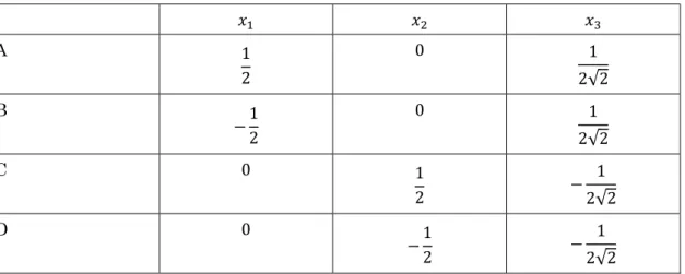
We can obtain the point of three vertexes as follow.
1
√3 0 , − 1 2√3
1
2 , − 1 2√3 −1
2 We can plot them as following figure.
Fig. 83. Two-dimensional plot of 3 points For the confirmation, we calculate the distances.
1
√3 0 − − 1 2√3
1
2 = √3
2 + −1 2 = 1
1
√3 0 − − 1 2√3 −1
2 = √3
2 + 1 2 = 1
− 1 2√3
1
2 − − 1 2√3 −1
2 = (0) + (1) = 1 We could obtain equilateral triangle without any loss of information.
As a result of selection of 2
−1
−1
as one of eigenvector, a vertex exists on vertical axis.
We can understand the three points form a flat from the result that one of the eigenvalue is 0.
Example 2 (quadrate)
Several cynics may say that it is trivial 3 points make a flat. We try to calculate the case of quadrate of which side is 1 in length.
Distance matrix is as follow.
𝑫 =
⎝
⎜
⎛ 0 1 1 0
√2 1 1 √2
√2 1 1 √2
0 1 1 0 ⎠
⎟
⎞
Square distance matrix is as follow.
𝑫𝟐= 0 1 1 0
2 1 2 1 1 2 1 2
0 1 1 0 Centralization
𝑮𝒏𝑫 𝑮𝒏 =
⎝
⎜
⎜
⎜
⎜
⎛ 3 4 −1
4
−1 4
3 4
−1 4 −1
4
−1 4 −1
4
−1 4 −1
4
−1 4 −1
4 3 4 −1
4
−1 4
3 4 ⎠
⎟
⎟
⎟
⎟
⎞ 0 1 1 0
2 1 1 2 2 1 1 2
0 1 1 0
⎝
⎜
⎜
⎜
⎜
⎛ 3 4 −1
4
−1 4
3 4
−1 4 −1
4
−1 4 −1
4
−1 4 −1
4
−1 4 −1
4 3 4 −1
4
−1 4
3 4 ⎠
⎟
⎟
⎟
⎟
⎞
=
−1 0 0 −1
1 0 0 1 1 0
0 1
−1 0 0 −1
⎝
⎜
⎜
⎜
⎜
⎛ 3 4 −1
4
−1 4
3 4
−1 4 −1
4
−1 4 −1
4
−1 4 −1
4
−1 4 −1
4 3 4 −1
4
−1 4
3 4 ⎠
⎟
⎟
⎟
⎟
⎞
=
−1 0 0 −1
1 0 1 0 0 1
0 1
−1 0 0 −1 Calculation to obtain eigenvalues from eigen equation.
−1 − 𝜆 0 0 −1 − 𝜆
1 0 0 1 1 0
0 1
−1 − 𝜆 0 0 −1 − 𝜆
= 0
(𝜆 + 1) − 2(𝜆 + 1) + 1 = 0 ((𝜆 + 1) − 1) = 0
𝜆(𝜆 + 2) = 0
𝜆 = 0 (𝑚𝑢𝑙𝑡𝑖𝑝𝑙𝑒 𝑟𝑜𝑜𝑡), 𝜆 = −2 (𝑚𝑢𝑡𝑖𝑝𝑙𝑒 𝑟𝑜𝑜𝑡) Calculation to obtain eigenvector belonging to eigenvalue 𝜆 = 0.
−1 0 0 −1
1 0 1 0 0 1
0 1
−1 0 0 −1
𝑥 𝑥𝑥 𝑥
= 0 𝑥 𝑥𝑥 𝑥
−𝑥 + 𝑥 = 0 𝑥 − 𝑥 = 0 From this
𝑥 = 𝑥 , 𝑥 = 𝑥 We select following vector as simplest eigenvector.
1 11 1
Calculation to obtain eigenvector belonging to eigenvalue 𝜆 = −2.
−1 0 0 −1
1 0 1 0 0 1
0 1
−1 0 0 −1
𝑥 𝑥𝑥 𝑥
= −2 𝑥 𝑥𝑥 𝑥 𝑥 + 𝑥 = 0
𝑥 + 𝑥 = 0 From this
𝑥 = −𝑥 , 𝑥 = −𝑥 We select following vector as simplest eigenvector.
1
−11
−1
Calculation of the other eigenvector belonging to eigenvalue𝜆 = 0.
We use condition for orthogonality to upper two vectors. Following inner products should be 0.
(𝑥 𝑥 𝑥 𝑥 ) 1 11 1
= 0
(𝑥 𝑥 𝑥 𝑥 ) 1
−11
−1
= 0
𝑥 + 𝑥 + 𝑥 + 𝑥 = 0 𝑥 + 𝑥 − 𝑥 − 𝑥 = 0
𝑥 = −𝑥 , 𝑥 = −𝑥 We select following vector as simplest eigen vector.
1
−11
−1
Calculation of the other eigenvalue belonging to eigen value 𝜆 = −2. We use condition for orthogonality to upper three vectors. Following inner products should be 0.
(𝑥 𝑥 𝑥 𝑥 ) 1 11 1
= 0
(𝑥 𝑥 𝑥 𝑥 ) 1
−11
−1
= 0
(𝑥 𝑥 𝑥 𝑥 ) 1
−11
−1
= 0
𝑥 + 𝑥 + 𝑥 + 𝑥 = 0 𝑥 + 𝑥 − 𝑥 − 𝑥 = 0 𝑥 − 𝑥 + 𝑥 − 𝑥 = 0 𝑥 = −𝑥 , 𝑥 = −𝑥 , 𝑥 = 𝑥 , 𝑥 = 𝑥
We select following vector as simplest eigenvector.
1
−1−1 1
We can obtain following matrix which diagonalize 𝑮𝒏𝑫 𝑮𝒏.
𝑷 =
1 1 1 −1
1 1
−1 −1 1 −1
−1 1
1 1 1 −1
𝑮𝒏𝑫 𝑮𝒏 =
−1 0 0 −1
1 0 1 0 0 1
0 1
−1 0 0 −1
For future convenience, we make orthogonalizing matrix to unit vector.
𝑷 =
⎝
⎜
⎜
⎜
⎜
⎛ 1 2
1 2 1 2 −1
2 1 2
1 2 1 2 −1
2
−1 2 −1
2
−1 2
1 2
1 2
1 2 1 2 −1
2⎠
⎟
⎟
⎟
⎟
⎞
𝑷 = 𝑷
𝜦 =
−2 0 0 −2
0 0 0 0 0 0
0 0
0 0 0 0 Diagonalization
−1 0 0 −1
1 0 1 0 0 1
0 1
−1 0 0 −1
= 𝑷𝜦𝑷 Using this
𝑮𝒏𝑫 𝑮𝒏 =
−1 0 0 −1
1 0 1 0 0 1
0 1
−1 0 0 −1
=
⎝
⎜
⎜
⎜
⎜
⎛ 1 2
1 2 1 2 −1
2 1 2
1 2 1 2 −1
2
−1 2 −1
2
−1 2
1 2
1 2
1 2 1 2 −1
2⎠
⎟
⎟
⎟
⎟
⎞ −2 0 0 −2
0 0 0 0 0 0
0 0
0 0 0 0
⎝
⎜
⎜
⎜
⎜
⎛ 1 2
1 2 1 2 −1
2
−1 2 −1
2
−1 2
1 2 1
2 1 2 1 2 −1
2 1 2 1
2 1 2 −1
2 ⎠
⎟
⎟
⎟
⎟
⎞
𝒁 =𝑮𝒏𝑫 𝑮𝒏
−2
= 1
−2
⎝
⎜
⎜
⎜
⎜
⎛ 1 2
1 2 1 2 −1
2 1 2
1 2 1 2 −1
2
−1 2 −1
2
−1 2
1 2
1 2
1 2 1 2 −1
2⎠
⎟
⎟
⎟
⎟
⎞ −2 0 0 −2
0 0 0 0 0 0
0 0
0 0 0 0
⎝
⎜
⎜
⎜
⎜
⎛ 1 2
1 2 1 2 −1
2
−1 2 −1
2
−1 2
1 2 1
2 1 2 1 2 −1
2 1 2 1
2 1 2 −1
2 ⎠
⎟
⎟
⎟
⎟
⎞
=
⎝
⎜
⎜
⎜
⎜
⎛ 1 2
1 2 1 2 −1
2 1 2
1 2 1 2 −1
2
−1 2 −1
2
−1 2
1 2
1 2
1 2 1 2 −1
2⎠
⎟
⎟
⎟
⎟
⎞ 1 0 0 1
0 0 0 0 0 0 0 0
0 0 0 0
⎝
⎜
⎜
⎜
⎜
⎛ 1 2
1 2 1 2 −1
2
−1 2 −1
2
−1 2
1 2 1
2 1 2 1 2 −1
2 1 2 1
2 1 2 −1
2 ⎠
⎟
⎟
⎟
⎟
⎞
Transform to the form of 𝑷𝜦𝟏𝟐𝜦𝟏𝟐𝑷 .
𝑷𝜦𝟏𝟐𝜦𝟏𝟐𝑷 =
⎝
⎜
⎜
⎜
⎜
⎛ 1 2
1 2 1 2 −1
2 1 2
1 2 1 2 −1
2
−1 2 −1
2
−1 2
1 2
1 2
1 2 1 2 −1
2⎠
⎟
⎟
⎟
⎟
⎞ 1 0 0 1
0 0 0 0 0 0 0 0
0 0 0 0
1 0 0 1
0 0 0 0 0 0 0 0
0 0 0 0
⎝
⎜
⎜
⎜
⎜
⎛ 1 2
1 2 1 2 −1
2
−1 2 −1
2
−1 2
1 2 1
2 1 2 1 2 −1
2 1 2 1
2 1 2 −1
2 ⎠
⎟
⎟
⎟
⎟
⎞
𝑷𝜦𝟏𝟐𝜦𝟏𝟐𝑷 =
⎝
⎜
⎜
⎜
⎜
⎛ 1 2
1 2 1 2 −1
2
−1 2
−1 2
−1 2 1 2 ⎠
⎟
⎟
⎟
⎟
⎞ 1 0 0 1
1 0 0 1
1 2
1 2 −1
2 −1 2 1
2 −1 2 −1
2 1 2
What we need is 𝑷𝜦𝟏𝟐.
𝑷𝜦𝟏𝟐=
⎝
⎜
⎜
⎜
⎜
⎛ 1 2
1 2 1 2 −1
2
−1 2
−1 2
−1 2 1 2 ⎠
⎟
⎟
⎟
⎟
⎞ 1 0 0 1 =
⎝
⎜
⎜
⎜
⎜
⎛ 1 2
1 2 1 2 −1
2
−1 2
−1 2
−1 2 1 2 ⎠
⎟
⎟
⎟
⎟
⎞
1 2
1 2 , 1
2 −1 2 , −1
2 −1 2 , −1
2 1 2
Fig.84. Two-dimensional plot of 4 vertexes
These vertexes form quadrate of which center is origin. We could understand that the es are distributing in 2-dimensinal space from the calculation of eigenvalues in which there are two vectors from four are λ = 0.
Example 3 (tetrahedron)
As an example of 3-dimensional data, we calculate tetrahedron of which lengths of sides are 1.
𝑫 = 0 1 1 0
1 1 1 1 1 1 1 1
0 1 1 0
𝑫𝟐= 0 1 1 0
1 1 1 1 1 1 1 1
0 1 1 0 Centralization.
𝑮𝒏𝑫 𝑮𝒏 =
⎝
⎜
⎜
⎜
⎜
⎛ 3 4 −1
4
−1 4
3 4
−1 4 −1
4
−1 4 −1
4
−1 4 −1
4
−1 4 −1
4 3 4 −1
4
−1 4
3 4 ⎠
⎟
⎟
⎟
⎟
⎞ 0 1 1 0
1 1 1 1 1 1 1 1
0 1 1 0
⎝
⎜
⎜
⎜
⎜
⎛ 3 4 −1
4
−1 4
3 4
−1 4 −1
4
−1 4 −1
4
−1 4 −1
4
−1 4 −1
4 3 4 −1
4
−1 4
3 4 ⎠
⎟
⎟
⎟
⎟
⎞
=
⎝
⎜
⎜
⎜
⎜
⎛
−3 4
1 4 1 4 −3
4 1 4 1
4 1 4 1
4 1
4 1 4 1 4 1
4
−3 4
1 4 1 4 −3
4⎠
⎟
⎟
⎟
⎟
⎞
⎝
⎜
⎜
⎜
⎜
⎛ 3 4 −1
4
−1 4
3 4
−1 4 −1
4
−1 4 −1
4
−1 4 −1
4
−1 4 −1
4 3 4 −1
4
−1 4
3 4 ⎠
⎟
⎟
⎟
⎟
⎞
=
⎝
⎜
⎜
⎜
⎜
⎛
−3 4
1 4 1 4 −3
4 1 4 1
4 1 4 1
4 1
4 1 4 1 4 1
4
−3 4
1 4 1 4 −3
4⎠
⎟
⎟
⎟
⎟
⎞
=1 4
−3 1 1 −3
1 1 1 1 1 1
1 1
−3 1 1 −3
Concerning
−3 1 1 −3
1 1 1 1 1 1
1 1
−3 1 1 −3
, we calculate eigenvalue.
−3 − 𝜆 0 0 −3 − 𝜆
1 0 0 1 1 0
0 1
−3 − 𝜆 0 0 −3 − 𝜆
= 0
(𝜆 + 3) − 2(𝜆 + 3) + 1 = 0 ((𝜆 + 3) − 1) = 0
(𝜆 + 3) = 1 (𝜆 + 3) = ±1
𝜆 = −4 (𝑚𝑢𝑙𝑡𝑖𝑝𝑙𝑒 𝑟𝑜𝑜𝑡), 𝜆 = −2 (𝑚𝑢𝑙𝑡𝑖𝑝𝑙𝑒 𝑟𝑜𝑜𝑡) We calculate eigenvectors belonging to eigen value 𝜆 = −4.
−3 1 1 −3
1 1 1 1 1 1
1 1
−3 1 1 −3
𝑥 𝑥𝑥 𝑥
= −4 𝑥 𝑥𝑥 𝑥
−3𝑥 + 𝑥 + 𝑥 + 𝑥 = −4𝑥 𝑥 − 3𝑥 + 𝑥 + 𝑥 = −4𝑥 𝑥 + 𝑥 − 3𝑥 + 𝑥 = −4𝑥 𝑥 + 𝑥 + 𝑥 − 3𝑥 = −4𝑥 From all equations
𝑥 + 𝑥 + 𝑥 + 𝑥 = 0 Simplest vector satisfying upper equation is as follow.
1
−10 0
Simplest orthogonal vector to upper vector satisfying the equation is as follow.
0 01
−1 We select these vectors as eigenvectors.
𝑽 = 1
−10 0
, 𝑽 = 0 01
−1
Calculation for eigenvectors belonging to eigenvalue 𝜆 = −2.
−3 1 1 −3
1 1 1 1 1 1
1 1
−3 1 1 1
𝑥 𝑥𝑥 𝑥
= −2 𝑥 𝑥𝑥 𝑥
−3𝑥 + 𝑥 + 𝑥 + 𝑥 = −2𝑥 𝑥 − 3𝑥 + 𝑥 + 𝑥 = −2𝑥 𝑥 + 𝑥 − 3𝑥 + 𝑥 = −2𝑥 𝑥 + 𝑥 + 𝑥 − 3𝑥 = −2𝑥
𝑥 = 𝑥 + 𝑥 + 𝑥 i 𝑥 = 𝑥 + 𝑥 + 𝑥 ii 𝑥 = 𝑥 + 𝑥 + 𝑥 iii 𝑥 = 𝑥 + 𝑥 + 𝑥 iv i − ii 𝑥 − 𝑥 = 𝑥 − 𝑥
𝑥 = 𝑥 Similarly from iii―iv,
𝑥 = 𝑥 From ii+iii,
𝑥 = −𝑥
From i+iv,
𝑥 = −𝑥
We select following vectors as simplest vector satisfying the condition.
𝑉 = 1
−11
−1
, 𝑉 ′ =
−1
−11 1
Space 𝑽 ,- 𝑽 - 𝑽 and Space 𝑽 ,- 𝑽 - 𝑽 ′ are in the relation of mirror image, and 𝑽 and 𝑽 ′ are oppositely oriented and is existing on the same line. We can combine 𝑽 ′ to 𝑽 .
𝑽 = 1
−10 0
, 𝑽 = 0 01
−1
, 𝑽 = 1
−11
−1
We transform them into unit vectors
⎝
⎜
⎜
⎛ 1
√2
− 1
√2 0 0 ⎠
⎟
⎟
⎞ ,
⎝
⎜
⎜
⎛ 0 0 1
√2
− 1
√2⎠
⎟
⎟
⎞ ,
⎝
⎜
⎜
⎜
⎜
⎛ 1 2 1 2
−1 2
−1 2⎠
⎟
⎟
⎟
⎟
⎞
Conclusively, the diagonalizing matrix of
−3 1 1 −3
1 1 1 1 1 1
1 1
−3 1 1 −3
is as follow.
𝑷 =
⎝
⎜
⎜
⎜
⎜
⎜
⎛ 1
√2 0 1
2
− 1
√2 0 1
2 0
0 1
√2
− 1
√2
−1 2
−1 2⎠
⎟
⎟
⎟
⎟
⎟
⎞
The eigenvalue of third eigenvector is (−2) + (−2) = −4.
𝜦 =
−4 0 0 0 −4 0 0 0 −4
−3 1 1 −3
1 1 1 1 1 1
1 1
−3 1 1 −3
= 𝑷𝜦𝑷𝑻 Using them.
𝑮𝒏𝑫 𝑮𝒏 =1 4
−3 1 1 −3
1 1 1 1 1 1
1 1
−3 1 1 −3
=1 4
⎝
⎜
⎜
⎜
⎜
⎜
⎛ 1
√2 0 1
2
− 1
√2 0 1
2 0
0 1
√2
− 1
√2
−1 2
−1 2⎠
⎟
⎟
⎟
⎟
⎟
⎞
−4 0 0 0 −4 0 0 0 −4
⎝
⎜
⎜
⎜
⎜
⎜
⎛ 1
√2 0 1
2
− 1
√2 0 1
2 0
0 1
√2
− 1
√2
−1 2
−1 2⎠
⎟
⎟
⎟
⎟
⎟
⎞