Neighborhood Parallel Simulated Annealing
Keiko Ando 1 , Mitsunori Miki 2 , and Tomoyuki Hiroyasu 2
1
Graduate School of Knowledge Engineering and Computer Science, Doshisha Univ., Kyoto, Japan. [email protected]
2
Department of Knowledge Engineering and Computer Science, Doshisha Univ., Kyoto, Japan. {mmiki@mail, tomo@is}.doshisha.ac.jp
1 Introduction
Simulated annealing(SA) is a method for solving combinatorial optimization problems. SA was formulated by Kirkpatrick et al., and its algorithm imitates physical annealing. It is very useful for solving several types of optimization problems with nonlinear functions and multiple local optima[1, 2, 3].
The advantages and disadvantages of SA are well summarized in [4].The most significant disadvantages are the difficulty in determining the appropri- ate parameters, and the long calculation time for determining the optimum solution. The neighborhood range and temperature are the important param- eters in SA. In combinatorial optimization problems, the neighborhood range can be determined by replacing two adjoining elements in solutions. Thus, a neighborhood range is decided automatically for every problem; therefore, the temperature schedule becomes the most important factor. On the other hand, when SA is applied to continuous optimization problems, a neighborhood range can be freely decided in the range of the Eucledean space. However, the appropriate neighborhood range is greatly dependent on the landscape of the objective function. Therefore, the control of the neighborhood range becomes very important when applying SA to a continuous optimization problem, but it is difficult to detremine a neighborhood range automatically in this case.
Some research has been carried out wherein the neighborhood range was adjusted adaptively according to the landscape of the objective function.
Corana’s method[6] controls the neighborhood range according to a land- scapes maintaining an acceptance ratio of 0.5. The authors proposed a new method called SA/AAN wherein the appropriate neighborhood range can be determined based on the arbitrary acceptance ratio. These methods do not require the tuning of their parameters for many problems; however, the target values of the acceptance ratio are necessary.
In this research, we propose a parameter-free SA method called Neigh-
borhood Parallel Simulated Annealing (NPSA). This method determines the
neighborhood range automatically and does not require the acceptance ratio
in order to adjust a neighborhood range.
2 Keiko Ando, Mitsunori Miki, and Tomoyuki Hiroyasu
2 NPSA
2.1 The NPSA concept
In NPSA, parallel processing is performed and neighborhood ranges are assigned during each process. The neighborhood ranges are self-adjusted through the exchange of neighborhood ranges between processors. Such an algorithm enables the exchange of the neighborhood ranges between proces- sors based on the energy of the solutions. The processor with a low energy is assigned a small neighborhood range, so that the solution can search locally.
On the other hand, the processor with a high energy is assigned a large neigh- borhood range, so that the solution can avoid the local minima. Thus, the processors cooperate and adjust neighborhood ranges as the search proceeds.
2.2 The NPSA algorithm
The NPSA algorithm is pictorially depicted in Fig. 1. The process followed in NPSA is described below.
1. Parallel processing is performed.
2. A different neighborhood is assigned during in each process.
3. SA is excecuted in parallel in each processor.
4. At every cooling cycle, the energy values(evaluation value) are gathered in one process.
5. The energy values are sorted, and the rank is determined based on the energy.
6. The neighborhood range is assigned according to the rank as follows.
Processor B is ranked 1; therefore, this processor’s neighborhood is de- termined to be the smallest. Processor D is ranked 4; therefore, this pro- cessor’s neighborhood is determined to be the biggest. The same logic is applied to the remaining cases.
7. Steps 3 to 6 are repeated.
Each processor has a different neighborhood.
Searching Area
Neighborhood range SA SA SA SA
E=30 E=10 E=100 E=300 Determine the rank
ԙ Ԙ Ԛ ԛ
SA SA SA Calculate Energy SA
A B C D
...
...
...
...
Fig. 1. NPSA algorithm
3 Effectiveness varification of the proposed method
3.1 Optimization problems
In order to exmine the search performance of the proposed method, two stan-
dard test functions are used, namely the Rastrigin and the Griewank func-
tions. The optimum solutions are located at the origin for the Rastrigin and
Neighborhood Parallel Simulated Annealing 3 Griewank functions, and the function values are 0, and its function value is also 0. Two, three, and five dimensions of these functions are used as test functions.
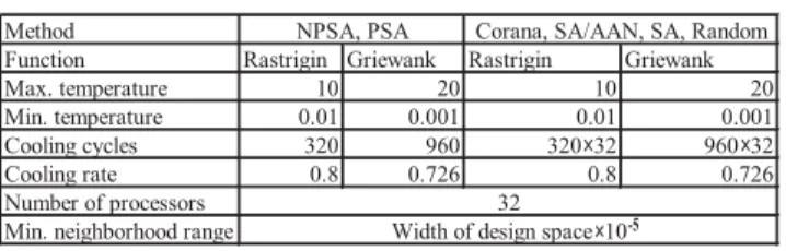
The parameters are indicated in Table 1. The number of both cooling cycles and parallel processors were set to 32. Thirty-two parallel processors are used in both NPSA and PSA, and the annealing step was set to the same value as that in sequential methods by setting the cooling cycle to 1/32 times.
Table 1. Parameters
Method
Function Rastrigin Griewank Rastrigin Griewank
Max. temperature 10 20 10 20
Min. temperature 0.01 0.001 0.01 0.001
Cooling cycles 320 960 320 32 960 32
Cooling rate 0.8 0.726 0.8 0.726
Number of processors Min. neighborhood range
Corana, SA/AAN, SA, Random NPSA, PSA
32 Width of design space 10
-5
3.2 Results and discussion
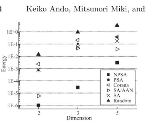
The minimum energy value obtained using the Rastrigin function is indi- cated in Fig. 2, while that using Griewank function is indicated in Fig. 3.
The comparison between the Random Search, Conventional SA(SA), Corana, SA/AAN, and NPSA methods in Fig. 2 and 3 clearly demonstrates the pro- posed method’s(NPSA) exceedingly superior performance on all dimensions.
We now consider the effectiveness of NPSA by compareing the energy histories of PSA, which is the standard method of SA, and NPSA, which demonstrates a superior performance. It is clear from Fig. 4 and 5 that NPSA yields a better solution and arrives at the optimum solution faster than PSA.
The neighborhood range selected can be considered as the reason for this.
This difference in performance stems from the variation of the neighbor- hood range. Fig. 6 shows the history of the neighborhood ranges. PSA main- tains range 1, which is the best range arrived at through extensive preliminary experimentation. On the other hand, NPSA utilizes the new adaptive mech- anism for assigning the neighborhood range. In Fig. 6, the solutions trapped in a local minima in the first stage; therefor, the neighborhood range become quite large. In the middle stage, the solution has converged on the global min- imum, and the neighborhood range has become increasingly smaller for local search. In the final stage, this mechanism can search the global optimum area.
Thus, NPSA can adaptively vary the neighborhood range as search process proceeds, thereby facility effective searching.
4 Conclusion
When simulated annealing is applied to a continuous optimized problem,
neighborhood range adjustment is indispensable. This research proposed the
NPSA method with a new neighborhood range generation mechanism that
eliminates unnecessary parameters. The proposed method is found to be very
effective for solving continuous optimization problems by SA.
4 Keiko Ando, Mitsunori Miki, and Tomoyuki Hiroyasu
Energy
Dimension 1E-6
1E-5 1E-4 1E-3 1E-2 1E-1 1E+0
2 3 5
NPSA PSA Corana SA/AAN SA Random
Fig. 2. energy value (Rastrigin function)
Energy
Dimension 1E-6
1E-5 1E-4 1E-3 1E-2 1E-1 1E+0
2 3 5
NPSA PSA Corana SA/AAN SA Random
Fig. 3. Energy value (Griewank func- tion)
0.0 0.2 0.4 0.6 0.8 1.0
1E-7 1E-6 1E-5 1E-4 1E-3 1E-2 1E-1 1E+0 1E+1 1E+2
Annealing steps
Energy
Best Energy Current Energy
104
Fig. 4. energy history of NPSA
References
1. Hajime Kita (1997) Simulated An- nealing. Japan Society for Fuzzy Theory and Intelligent Informatics, Vol. 9, No. 6, pp. 870-875
2. Aarts, E.(1989) Simulated Anneal- ing and Boltzmann Machines: A
Best Energy Current Energy
Energy
Annealing steps
0.0 0.2 0.4 0.6 0.8 1.0
1E-4 1E-3 1E-2 1E-1 1E+0 1E+1 1E+2
104
Fig. 5. energy history of PSA
0.0 0.2 0.4 0.6 0.8 1.0
1E-5 1E-4 1E-3 1E-2 1E-1 1E+0 1E+1
Neighborhood range
Annealing steps
NPSA PSA
104