Learning low-rank output kernels

Learning low-rank output kernels

Francesco Dinuzzo [email protected] Max Planck Institute for Intelligent Systems

Spemannstrasse 38, 72076 T¨ ubingen, Germany

Kenji Fukumizu [email protected]

The Institute of Statistical Mathematics 10-3 Midori-cho,

Tachikawa, Tokyo 190-8562 Japan

Editor: Chun-Nan Hsu and Wee Sun Lee

Abstract

Output kernel learning techniques allow to simultaneously learn a vector-valued function and a positive semidefinite matrix which describes the relationships between the outputs.

In this paper, we introduce a new formulation that imposes a low-rank constraint on the output kernel and operates directly on a factor of the kernel matrix. First, we investigate the connection between output kernel learning and a regularization problem for an architecture with two layers. Then, we show that a variety of methods such as nuclear norm regularized regression, reduced-rank regression, principal component analysis, and low rank matrix approximation can be seen as special cases of the output kernel learning framework. Finally, we introduce a block coordinate descent strategy for learning low-rank output kernels.

Keywords: Output kernel learning, learning the kernel, RKHS, coordinate descent

1. Introduction

Methods for learning vector-valued functions are becoming popular subjects of study in ma- chine learning, motivated by applications to multi-task learning, multi-label and multi-class classification. In these problems, selecting a model that correctly exploits the relationships between the different output components is crucial to ensure good learning performances.

Within the framework of regularization in reproducing kernel Hilbert spaces (RKHS) of vector-valued functions (Aronszajn, 1950; Micchelli and Pontil, 2005), one can directly encode relationships between the outputs by choosing a suitable operator-valued kernel. A simple and well studied model assumes that the kernel can be decomposed as the product of a scalar positive semidefinite kernel on the input space (input kernel), and a linear operator on the output space (output kernel ), see e.g. (Evgeniou et al., 2005; Bonilla et al., 2008;

Caponnetto et al., 2008; Baldassarre et al., 2010; Dinuzzo et al., 2011). Covariance functions (kernels) of this form have been also studied in geostatistics, in the context of the so-called intrinsic coregionalization model, see e.g. (Goovaerts, 1997; Alvarez and Lawrence, 2011).

The choice of the output kernel may significantly influence learning performance. When

prior knowledge is not sufficient to fix the output kernel in advance, it is necessary to adopt

automatic techniques to learn it from the data. A multiple kernel learning approach has

been proposed by Zien and Ong (2007), while Bonilla et al. (2008) propose to choose the

output kernel by minimizing the marginal likelihood within a Bayesian framework. Recently, a methodology to learn simultaneously a vector-valued function in a RKHS and a kernel on the output space has been proposed (Dinuzzo et al., 2011). Such a technique is based on the optimization of a non-convex functional that, nevertheless, can be globally optimized in view of invexity (Mishra and Giorgi, 2008). The method of Dinuzzo et al. (2011) directly operates on the full output kernel matrix which, in general, is full-rank. However, when the dimensionality of the output space is very high, storing and manipulating the full matrix may not be efficient or feasible.

In this paper, we introduce a new output kernel learning method that enforces a rank constraint on the output kernel and directly operates on a factor of the kernel matrix. In section 2, we recall some preliminary results about RKHS of vector valued functions and decomposable kernels, and introduce some matrix notations. In section 3, we introduce the low-rank output kernel learning model and the associated optimization problem. In section 4, we show that the proposed output kernel learning problem can be seen as the kernelized version of nuclear norm regularization. In view of such connection, a variety of methods such as reduced-rank regression (Anderson, 1951; Izenman, 1975; Reinsel and Velu, 1998), principal component analysis (Jolliffe, 1986), and low rank matrix approximation (Eckart and Young, 1936) can be seen as particular cases. In section 5 we develop an optimization algorithm for output kernel learning based on a block coordinate descent strategy. Finally, in section 6, performances of the algorithm are investigated using synthetic multiple time series reconstruction datasets, and compared with previously proposed methods. In Appendix A, we discuss an alternative formulation of the low rank output kernel learning problem and derive a suitable optimality condition. All the proofs are given in Appendix B.

2. Preliminaries

In sub-section 2.1, we review basic definitions regarding kernels and reproducing kernel Hilbert spaces of vector-valued functions (Micchelli and Pontil, 2005), and then introduce a class of decomposable kernels that will be the focus of the paper. In sub-section 2.2, we introduce some matrix notations needed in the paper.

2.1. Reproducing Kernel Hilbert Spaces

Let X denote a non-empty set and Y a Hilbert space with inner product h·, ·i

. Throughout the paper, all Hilbert spaces are assumed to be real. Let L(Y ) denote the space of bounded linear operators from Y into itself.

Definition 1 (Positive semidefinite Y-kernel) A symmetric function H : X × X → L(Y) is called positive semidefinite Y-kernel on X if, for any natural number `, the following holds

`

X

i=1

`

X

j=1

hy

, H (x

, x

)y

i

≥ 0, ∀(x

, y

) ∈ (X , Y) .

It is often convenient to consider the function obtained by fixing one of the two arguments

of the kernel to a particular point.

Definition 2 (Kernel section) Let H denote a Y-kernel on X . A kernel section centered on x ¯ ∈ X is a map H

: X → L(Y) defined as

H

(x) = H(¯ x, x).

The class of positive semidefinite Y -kernels can be associated with a suitable family of Hilbert spaces of vector-valued functions.

Definition 3 (RKHS of Y-valued functions) A Reproducing Kernel Hilbert Space of Y-valued functions g : X → Y is a Hilbert space H such that, for all x ∈ X , there exists C

∈ R such that

kg(x)k

≤ C

kgk

, ∀g ∈ H.

It turns out that every RKHS of Y-valued functions H can be associated with a unique positive semidefinite Y -kernel H, called the reproducing kernel, such that the following reproducing property holds:

hg(x), yi

= hg, H

yi

, ∀(x, y, g) ∈ (X , Y, H) .

Conversely, given a positive semidefinite Y-kernel H on X , there exists a unique RKHS of Y-valued functions defined over X whose reproducing kernel is H. The standard definition of positive semidefinite scalar kernel and RKHS (of real-valued functions) can be recovered by letting Y = R . The following definition introduces a specific class of Y-kernels that will be the focus of this paper.

Definition 4 (Decomposable Kernel) A positive semidefinite Y-kernel on X is called decomposable if it can be written as

H

= K · L,

where K is a positive semidefinite scalar kernel on X and L : Y → Y is a self-adjoint positive semidefinite operator, i.e.

hy, Lyi

≥ 0, ∀y ∈ Y .

In the previous definition, K takes into account the similarity between the inputs (input kernel ), and L measures the similarity between the output’s components (output kernel ).

2.2. Matrix notation

The identity matrix is denoted as I, the vector of all ones is denoted by e. For any matrix A, A

denote the transpose, tr(A) the trace, rank(A) the rank, rg(A) the range, and A

the Moore-Penrose pseudo-inverse. For any pair of matrices of the same size A, B, let hA, Bi

:= tr(A

B) denote the Frobenius inner product, and kAk

:= p

hA, Ai

the induced norm. In addition, kAk

:= tr

A

A

denote the nuclear norm, which coincides with the trace when A is square symmetric and positive semidefinite. The symbols

⊗, , and denote the Kronecker product, the Hadamard (element-wise) product, and the element-wise division, respectively. Finally, let S

denote the closed cone of positive semidefinite matrices or order m, and

S

=

A ∈ S

: rank(A) ≤ p ⊆ S

the set of positive semidefinite matrices whose rank is less than or equal to p.

3. Low-rank output kernel learning

Let Y = R

, and let H denote an RKHS of Y-valued functions whose reproducing kernel is decomposable (see Definition 4). Given a set of ` input-output data pairs (x

, y

) ∈ X × Y, and a positive real number λ > 0, consider the following problem (low-rank output kernel learning ):

min

L∈S^m,p+

"

min

`

X

i=1

ky

− g(x

)k

2λ + kgk

2 + tr(L) 2

!#

. (1)

First of all, application of the representer theorem (Kimeldorf and Wahba, 1971; Sch¨ olkopf et al., 2001; Micchelli and Pontil, 2005) to the inner minimization problem of (1) yields

g = L

`

X

i=1

c

K

! .

Then, by introducing the input kernel matrix K ∈ S

such that K

= K(x

, x

), and matrices Y, C ∈ R

such that

Y = (y

, . . . , y

)

, C = (c

, . . . , c

)

, problem (1) can be rewritten as

min

L∈S^m,p+

min

C∈R^`×m

kY − KCLk

2λ + hC

KC, Li

2 + tr(L)

2

. (2)

Although the objective functional of (1) is separately convex with respect to C and L, it is not jointly (quasi)-convex with respect to the pair (C, L). Nevertheless, by using techniques similar to Dinuzzo et al. (2011), is it possible to prove invexity, so that stationary points are global minimizers. Unfortunately, in presence of the rank constraint, stationary points are not guaranteed to be feasible points. In Appendix A, we derive a sufficient condition for global optimality based on a reformulation of problem (2).

3.1. Output kernel learning as a kernel machine with two layers

In this subsection, we present an alternative interpretation of problem (1). Such formulation allows us to apply the model to data compression and visualization problems, and will be also useful for optimization purposes. Consider a map g : X → Y of the form:

g(x) = (g

◦ g

)(x),

where g

: X → R

is a non-linear vector-valued function, and g

: R

→ Y is a linear

function. One can interpret g

as a map that performs a non-linear feature extraction or

dimensionality reduction, while the operator g

linearly combines the extracted features to

produce the output vector. In particular, assume that g

belongs to an RKHS H

of vector

valued functions whose kernel is decomposable as H = K ·I, and g

belongs to the space H

of linear operators of the type g

(z) = Bz, endowed with the Hilbert-Schmidt (Frobenius) norm. Consider the following regularization problem

g

min

"

g

min

`

X

i=1

ky

− (g

◦ g

)(x

)k

2λ + kg

k

1

2 + kg

k

2

2

!#

(3) According to the representer theorem for vector-valued functions, the inner minimization problem admits a solution of the form

g

=

`

X

i=1

a

K

and thus we have

g = B

`

X

i=1

a

K

! .

By introducing matrices K, Y as in the previous section, and letting A ∈ R

such that A = (a

, . . . , a

)

,

the regularization problem can be rewritten as

B∈

min

min

A∈R^`×p

Q(A, B), (4)

where

Q(A, B) := kY − KAB

k

2λ + hA, KAi

2 + kBk

2 The following result shows that problems (1) and (3) are equivalent.

Theorem 5 The optimal solutions g for problems (1) and (3) coincide.

3.2. Kernelized auto-encoder

In general, if the output data of problem (3) coincide with the inputs, i.e. y

= x

, the model can be seen as a kernelized auto-encoder with two layers, where the first layer g

performs a non-linear data compression, and the second-layer g

linearly decompresses the data. The compression ratio can be controlled by simply choosing the value of p. Alternatively, if the goal is data visualization in, say, two or three dimensions, one can simply set p = 2 or p = 3.

Kernel PCA (Sch¨ olkopf et al., 1998) is another related technique which uses positive

semidefinite kernels to perform non-linear feature extraction, and can be also interpreted

as an auto-encoder in the feature space. A popular application of kernel PCA is pattern

denoising, which requires the non-linear extraction of features followed by the solution of

a pre-image problem (Sch¨ olkopf et al., 1999). Observe that the kernelized auto-encoder

obtained by solving (3) differs from kernel PCA, since it minimizes a reconstruction error

in the original input space, and also introduces a suitable regularization on the non-linear

feature extractor. Differently from kernel PCA, the kernel machine with two layers discussed

in this section performs non-linear denoising without requiring the solution of a pre-image

problem.

4. A kernelized nuclear norm regularization problem

The following result shows the connection between problem (2) and a kernelized nuclear norm regularization problem with rank constraint.

Lemma 6 If Θ solves the following problem:

min

Θ∈R^`×m

kY − KΘk

2λ + tr

Θ

KΘ

, subject to rank(Θ) ≤ p, (5) then the pair

L = Θ

KΘ

, C = L

Θ, is an optimal solution of problem (2).

4.1. Special cases

In this subsection, we show that a variety of techniques such as nuclear norm regularization, reduced-rank regression, principal component analysis, and low-rank matrix approximation can be all seen as particular instances of the low-rank output kernel learning framework.

4.1.1. Linear input kernel

Let X ∈ R

denote a data matrix, and assume that the input kernel is linear:

K = XX

.

Then, letting Φ = X

Θ, problem (5) reduces to nuclear norm regularization with a rank constraint:

min

Φ∈R^`×m

kY − XΦk

2λ + kΦk

, subject to rank(Φ) ≤ p.

Indeed, the optimal Φ for this last problem must automatically be in the range of X

, see e.g. (Argyriou et al., 2009, Lemma 21). Observe that the nuclear norm regularization already enforces a low rank solution (Fazel et al., 2001). Therefore, for sufficiently large values of λ, the rank constraint is not active. On the other hand, when λ → 0

the solution of the previous problem converges to the reduced-rank regression solution:

min

Φ∈R^`×m

kY − XΦk

, subject to rank(Φ) ≤ p.

If Y = X, and X is centered, then we obtain principal component analysis:

min

Φ∈R^`×m

kX (I − Φ) k

, subject to rank(Φ) ≤ p.

Indeed, the optimal solution Φ of this last problem coincides with the projection operator over the subspace spanned by the first p principal components of X. In all these linear problems, the output kernel L is simply given by

L = Φ

Φ

.

4.1.2. Low-rank matrix approximation

For any non-singular input kernel matrix K, letting Θ = K

Z, the solution of (5) for λ → 0

tends to the low-rank matrix approximation solution:

min

Z∈R^`×m

kY − Zk

, subject to rank(Z) ≤ p.

The optimal Z coincides with a reduced singular value decomposition of Y (Eckart and Young, 1936).

5. Block coordinate descent for low-rank output kernel learning

In this section, we introduce an optimization algorithm (Algorithm 1) for solving problem (2) based on a block coordinate descent strategy. In particular, we consider the equivalent formulation (4), and alternate between optimization with respect to the two factors A and B. First of all, we assume that an eigendecomposition of the input kernel matrix K is available:

K = U

diag {λ

} U

.

Observe that the eigendecomposition can be computed once for all at the beginning of the optimization procedure.

5.1. Sub-problem w.r.t matrix A

When B is fixed in equation (4), the optimization with respect to A is a convex quadratic problem. A necessary and sufficient condition for optimality is

0 = ∂Q

∂A = − K Y − KAB

B

λ + KA

A sufficient condition is obtained by choosing A as the unique solution of the linear matrix equation

KA(B

B) + λA = YB.

Now, given the eigendecomposition

B

B = U

diag {λ

} U

, we have

A = U

VU

, where

V = Q λ

λ

+ λee

, Q = U

YBU

.

As shown in the following, during the coordinate descent procedure it is not necessary to

explicitly compute A. In fact, it is sufficient to compute V as in lines 5-7 of Algorithm 1.

5.2. Sub-problem w.r.t matrix B

For any fixed A, the sub-problem with respect to B is quadratic and strongly convex. The unique solution is obtained by setting

0 = ∂Q

∂B = − Y − KAB

KA

λ + B,

which can be rewritten as

B = Y

KA A

K

A + λI

.

Now, assume that A is optimized as in the previous subsection. Then, after some manipu- lations, taking into account the eigendecomposition of K and B

B, the update for B can be reduced to lines 9-10 of Algorithm 1.

5.3. Practical aspects

The solution in correspondence with different values of the regularization parameter λ can be computed efficiently by using a warm start procedure: the output kernel is initialized by using the result of the previous optimization, while moving from the highest value of the regularization parameter to the lowest. For each value of λ, we stop the coordinate descent procedure by checking whether the Frobenius norm of the variation of B from an iteration to the next is lower than a specified tolerance.

Observe that the eigenvectors of the input kernel matrix are used only outside the main loop of Algorithm 1, to properly rotate the outputs, and to reconstruct the factor A. The eigendecomposition of K can be computed once for all the values of the regularization pa- rameter: standard algorithms require O(`

) operations. The two key steps in each iteration of Algorithm 1 are the computation of the eigendecomposition in line 5 and the solution of the linear system in line 10. They can be both performed in O max{p

m, p

}

operations.

The memory required to store all the matrices scales as O(max{mp, `

}).

If the number of outputs m is very large, one can choose low values of p to control both computational complexity and memory requirements. On the other hand, if there are no limitations in memory and computation time, one could set p = m and use only λ to control the complexity of the model. By doing this, one is also guaranteed to obtain the global minimizer of the optimization problem. Notice that the parameters p and λ both control the rank of the resulting model.

6. Experiments: reconstruction of multiple signals

We apply low rank output kernel learning to reconstruct and denoise multiple signals. We

present two experiments. In the first experiment, we compare the learning performances of

Algorithm 1 with previously proposed techniques. Also, we investigate the dependence of

learning performances and training time on the rank parameter. In the second experiment,

we demonstrate that low rank output kernel learning scales well to datasets with a very

large number of outputs, whereas full-rank techniques cannot be applied anymore. All the

experiments have been run in a MATLAB environment with an Intel i5 CPU 2.4 GHz, 4

GB RAM.

Algorithm 1 Low-rank output kernel learning with block-wise coordinate descent

1: Compute eigendecomposition: K = U

diag {λ

} U

2: B ← I

3: Y e ← U

Y

4: repeat

5: Compute eigendecomposition: B

B = U

diag {λ

} U

6: Q ← YBU e

7: V ← Q λ

λ

+ λee

8: B

← B

9: E ← diag {λ

} V

10: B ← Y e

E E

E + λI

U

11: until kB − B

k

≥ δ

12: A ← U

VU

First of all, we generated 50 independent realizations Z

, (k = 1, . . . , 50) of a Gaussian Process on the interval [−1, 1] of the real line with zero-mean and covariance function

K(x

, x

) = exp(−10|x

− x

|).

We then generated m new processes U

as U

=

50

X

k=1

B

Z

,

where the mixing coefficients B

are independently drawn from a uniform distribution on the interval [0, 1]. Output data have been generated by sampling the processes U

in cor- respondence with 200 uniformly spaced input points in the interval [−1, 1], and corrupting them by adding a zero-mean Gaussian noise with a signal to noise ratio of 1:1.

6.1. Experiment 1

In the first experiments, we have set m = 200, and randomly extracted ` = 100 samples to be used for training, using the remaining 100 for tuning the regularization parameter λ. The results of method (1) are compared with the baseline obtained by fixing the output kernel to the identity, and the method of Dinuzzo et al. (2011) which uses a squared Frobenius-norm regularization on the output kernel. For each value of the rank parameter p = 1, . . . , m, the solution is computed for 25 logarithmically spaced values of the regularization parameter λ in the range

λ ∈

10

α, α

, α =

q

kY

KYk

.

In view of Lemma 8 in Appendix A, the optimal output kernel L is null for λ > α. For each

value of p, we used the warm start procedure (see subsection 5.3) for computing the solution

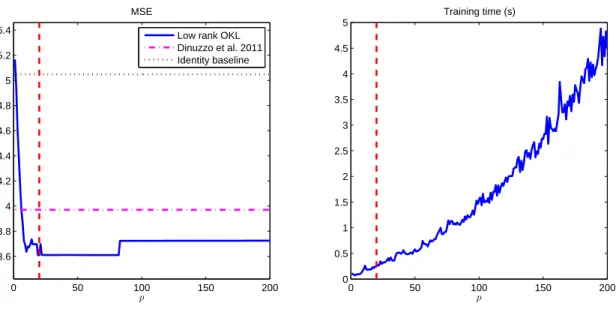
in correspondence with different values of the regularization parameter. Figure 1 reports the

MSE (mean squared error) on the left panel and the training time to compute the solution

for all the values of λ on the right panel, as a function of the rank parameter p. In terms of

0 50 100 150 200 3.6

3.8 4 4.2 4.4 4.6 4.8 5 5.2 5.4

p MSE

Low rank OKL Dinuzzo et al. 2011 Identity baseline

0 50 100 150 200

0 0.5 1 1.5 2 2.5 3 3.5 4 4.5 5

p Training time (s)

Figure 1: Experiment 1: The continuous lines represent the MSE (left panel) and training time (right panel) of Algorithm 1, as a function of the rank p. In the left panel, the horizontal baseline obtained by fixing the output kernel to the identity is dotted, while the performance of the method of (Dinuzzo et al., 2011) is dash-dotted.

The vertical dashed line corresponds to the value of p that minimizes MSE.

reconstruction error, the output kernel learning method (1) outperforms both the baseline model obtained by fixing L = I, and the Frobenius-norm regularization method, within a broad range of parameter p. The best performances are observed in correspondence with low values of the rank parameter (the vertical line corresponds to p = 20). Finally, from the right panel of Figure 1, one can observe the dependence of the training time on p. In particular, observe that the training time in correspondence with the best low rank model is reduced by more than an order of magnitude with respect to the full rank model.

6.2. Experiment 2

Within the same setting of the previous subsection, this time we generated m = 10

pro-

cesses U

. Again, we randomly choose 100 samples from the uniform grid to be used for

training and measure learning performances using the MSE (mean squared error). Observe

that in this case it is not possible to learn a full-rank output kernel matrix since it would

not fit into the memory. For the same reason, the method of Dinuzzo et al. (2011) (that

store the full matrix L) cannot be applied. Therefore, this time we fixed the rank parameter

p = 50, and report performances of the Algorithm 1 for 25 different values of the regulariza-

tion parameter chosen on a logarithmic scale. Performances are compared with the baseline

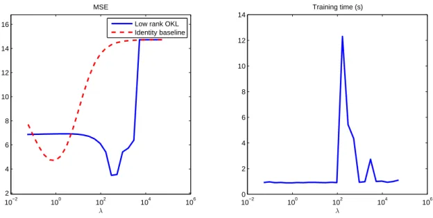
obtained by fixing L = I. From the left panel of Figure 2, we see that the low rank output

kernel performs better than the identity. The overall training time to compute the solution

of (1) for the 25 values of the regularization parameter is about 45 seconds. From the right

10⁻² 10⁰ 10² 10⁴ 10⁶ 2

4 6 8 10 12 14 16

λ MSE

Low rank OKL Identity baseline

10⁻² 10⁰ 10² 10⁴ 10⁶

0 2 4 6 8 10 12 14

λ Training time (s)

Figure 2: Experiment 2: The continuous lines represent the Mean Squared Error (left panel) and training time (right panel) of Algorithm 1, as a function of the regularization parameter λ. In the left plot, the baseline obtained by fixing the output kernel to the identity is dashed. In the right plot, the training time refers to an iteration of the warm-start procedure (see subsection 5.3).

panel of Figure 2, we can see that most of the computation time (using the warm-start procedure described in subsection 5.3) is spent in correspondence with intermediate values of λ. These values of λ also correspond to the best reconstruction performances. The right panel of Figure 2 also shows that the warm-start procedure does a good job at exploiting the continuity of the solution along a regularization path.

7. Conclusions

We have presented a new regularization-based methodology to learn low rank output kernels.

The new model encodes the assumption that the output components of the vector-valued function to be learned lie on a low-dimensional subspace. We have shown that the proposed framework can be interpreted as a kernel machine with two layers as well as the kernelized counterpart of nuclear norm regularization. Finally, we have developed an effective block coordinate descent technique to solve the proposed optimization problem. By manipulating only low-rank matrices, the new approach allows to limit memory requirements and improve performances with respect to previous techniques.

Appendix A. Optimality condition

Observe that the inner optimization problem in (2) is an unconstrained quadratic mini-

mization with respect to C. By eliminating C from the objective functional and letting

y = vec(Y), where vec(·) denotes the vectorization operator, we obtain the following prob- lem in L only

min

L∈S^m,p+

y

(L ⊗ K + λI)

y

2 + tr(L)

2

!

. (6)

Problem (6) is of the form

min

L∈S^m,p+

f (L), (7)

where f is a differentiable convex functional. Observe that, although the objective functional is convex, the feasible set is non-convex for p < m. Equivalently, problem (7) can be rewritten as an unconstrained minimization of a non-convex functional:

B∈

min

f (BB

). (8)

Now, letting

G(B) = ∂f BB

+ ∂f BB

2 ,

we have the following result.

Lemma 7 If B

is a global minimizer for (8), then

G(B

)B

= 0. (9)

Conversely, if (9) holds and, in addition, we have

G(B

) ∈ S

, (10)

then B

is a global minimizer for (8).

The following result specializes the more general result of Lemma 7 to problem (6).

Lemma 8 If L = BB

is an optimal solution of problem (6), then there exists C ∈ R

such that

KCL + λC = Y, (11)

C

KC

B = B, (12)

Conversely, if (11)-(12) hold and, in addition, we have

kC

KCk

≤ 1, (13)

then L is an optimal solution of problem (6).

A corollary of Lemma 8 is the following: if kY

KYk

≤ λ

, then L = 0 is an optimal solution of problem (6). To see this, it suffices to set C = Y/λ. Another simple observation is that, in view of (12), the rank of any optimal L is always less or equal than the rank of K. These two observations imply that the range of parameters λ and p, which define the low-rank output kernel learning algorithm, can be restricted as follows:

0 < λ ≤ q

kY

KYk

, 0 < p ≤ min {rank(K), m}

without any loss of generality.

Appendix B. Proofs

Proof [of Theorem 5] First of all, we show that problems (2) and (4) are equivalent.

Consider problem (2) and observe that, in view of the rank constraint, we have the decom- position L = BB

, where B ∈ R

. By letting

A = CB, (14)

problem (2) boils down to (4). Conversely, take an optimal A ∈ R

for problem (4), and observe that it admits a unique decomposition of the form

A = CB + U, UB

= 0.

We have

KAB

= KCBB

= KCL, and

hA, KAi

2 = hU, KUi

2 + hC

KC, Li

2 ≥ hC

KC, Li

2 .

It follows that we can set U = 0, so that A can be written as in (14) without any loss of generality. Finally, in view of (14), the optimal g for problems (1) and (3) coincide.

Proof [of Lemma 6] Letting Θ = CL, problem (2) can be rewritten as min

Θ∈R^`×m

"

kY − KΘk

2λ + min

L∈S^m,p+

hΘ

KΘ, L

i

2 + tr(L)

2 #

, subject to rg(Θ) ⊆ rg(L).

Now, it turns out that a closed-form solution of the inner minimization problem is given by L = Θ

KΘ

.

Indeed, such a solution is the only stationary point of the unconstrained functional, and also satisfies the constraints, provided that

rank(Θ) = rank(L) ≤ p.

By plugging the expression of L into the objective functional, we obtain problem (5).

Proof [of Lemma 7] Let

g(B) = f BB

, and observe that

vec(∇g(B)) = 2vec(G(B)) (B ⊗ I) = vec(2G(B)B), so that

∇g(B) = 2G(B)B.

Since g is differentiable, every global minimizer must be a stationary point, therefore equa- tion (9) follows. Now, assume that (9) and (10) holds. Then, by convexity of f we have

g(B

) − g(B) = f B

B

− f BB

≤ h∇f B

B

, B

B

− BB

i

= hG(B

), B

B

− BB

i

= −hG(B

), BB

i

= −tr B

G(B

)B

≤ 0, so that

g(B

) ≤ g(B), ∀B ∈ R

, and B

is a global minimizer.

Proof [of Lemma 8] Apply Lemma 7 to the objective functional of problem (6). It suffices to observe that G(B) can be expressed as

G(B) = 1

2 I − C

KC ,

where C satisfies the linear matrix equation (11). Then, conditions (9)-(10) boil down to (12)-(13), respectively.

References

M. A. Alvarez and N. D. Lawrence. Computationally efficient convolved multiple output Gaussian processes. Journal of Machine Learning Research, 12:1459–1500, 2011.

T. W. Anderson. Estimating linear restrictions on regression coefficients for multivariate normal distributions. Annals of Mathematical Statistics, 22:327–351, 1951.

A. Argyriou, C. A. Micchelli, and M. Pontil. When is there a representer theorem? Vector versus matrix regularizers. Journal of Machine Learning Research, 10:2507–2529, 2009.

N. Aronszajn. Theory of reproducing kernels. Transactions of the American Mathematical Society, 68:337–404, 1950.

L. Baldassarre, L. Rosasco, A. Barla, and A. Verri. Vector field learning via spectral filtering.

In Machine Learning and Knowledge Discovery in Databases, volume 6321, pages 56–71.

Springer, 2010.

E. Bonilla, K. Ming Chai, and C. Williams. Multi-task Gaussian process prediction. In J.C. Platt, D. Koller, Y. Singer, and S. Roweis, editors, Advances in Neural Information Processing Systems, pages 153–160. MIT Press, Cambridge, MA, 2008.

A. Caponnetto, C. A. Micchelli, M. Pontil, and Y. Ying. Universal multi-task kernels.

Journal of Machine Learning Research, 9:1615–1646, 2008.

F. Dinuzzo, C. S. Ong, P. Gehler, and G. Pillonetto. Learning output kernels with block co- ordinate descent. In Proceedings of the 28th Annual International Conference on Machine Learning, Bellevue, WA, USA, 2011.

C. Eckart and G. Young. The approximation of one matrix by another of lower rank.

Psychometrika, (1):211–218, 1936.

T. Evgeniou, C. A. Micchelli, and M. Pontil. Learning multiple tasks with kernel methods.

Journal of Machine Learning Research, 6:615–637, 2005.

M. Fazel, H. Hindi, and S. Boyd. A rank minimization heuristic with application to mini- mum order system approximation. In Proceedings of the American Control Conference, volume 6, pages 4734–4739, Arlington, Virginia, June 2001.

P. Goovaerts. Geostatistics For Natural Resources Evaluation. Oxford University Press, USA, 1997.

A. J. Izenman. Reduced-rank regression for the multivariate linear model. Journal of Multivariate Analysis, 5(2):248–264, 1975.

I. T. Jolliffe. Principal Component Analysis. Springer, New York, NY, USA, 1986.

G. Kimeldorf and G. Wahba. Some results on Tchebycheffian spline functions. Journal of Mathematical Analysis and Applications, 33(1):82–95, 1971.

C. A. Micchelli and M. Pontil. On learning vector-valued functions. Neural Computation, 17:177–204, 2005.

S. K. Mishra and G. Giorgi. Invexity and optimization. Nonconvex Optimization and Its Applications. Springer, Dordrecht, 2008.

G. H. Reinsel and R. P. Velu. Multivariate reduced rank regression: theory and applications.

Springer, New York, 1998.

B. Sch¨ olkopf, A. J. Smola, and K-R M¨ uller. Nonlinear component analysis as a kernel eigenvalue problem. Neural Computation, 10(5):1299–1319, 1998.

B. Sch¨ olkopf, S. Mika, C.J.C. Burges, P. Knirsch, K.-R. M¨ uller, G. R¨ atsch, and A.J. Smola.

Input space versus feature space in kernel-based methods. IEEE Transactions on Neural Networks, 10(5):1000 –1017, sep 1999.

B. Sch¨ olkopf, R. Herbrich, and A. J. Smola. A generalized representer theorem. Neural Networks and Computational Learning Theory, 81:416–426, 2001.

A. Zien and C. S. Ong. Multiclass multiple kernel learning. In Proceedings of the 24th

international conference on Machine learning, pages 1191–1198, 2007.