(1). The exact order of the likelihood ratio of multilayer perceptrons is derived, and a new regularization scheme is proposed to overcome the strong overÞtting.

(1)

2001年情報論的学習理論ワークショップ

2001 Workshop on Information-Based Induction Sciences (IBIS2001)

Tokyo, Japan, July 30 - August 1, 2001.

局所錐型モデルの漸近理論とそのニューラルネットへの応用 Asymptotic Theory of Locally Conic Models and its Applications to

Neural Networks

福水健次^∗

Kenji Fukumizu

Abstract: Multilayer neural networks have a problem of unidentiÞability in its parameter- ization. If a network has surplus hidden units to realize a target function, the parameters to give the function consist of a high dimensional subset. Many of usual statistical views fail in such cases. This paper discusses the likelihood ratio of the maximum likelihood es- timation in unidentiÞable cases, using the framework of locally conic models. We derive a suﬃcient condition that the likelihood ratio has a larger order than usual O

_p

(1). The exact order of the likelihood ratio of multilayer perceptrons is derived, and a new regularization scheme is proposed to overcome the strong overÞtting.

Keywords: Neural network, Maximum likelihood estimation, UnidentiÞability, Locally conic model, Regularization

1 Introduction

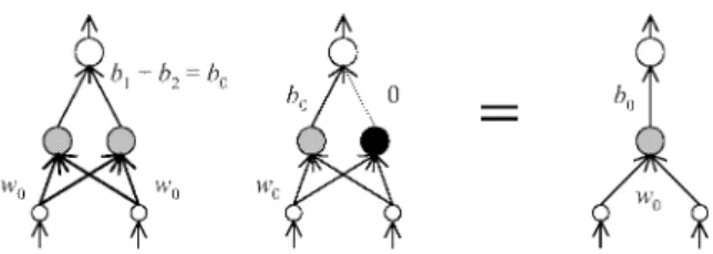
In a multilayer neural network model with H hidden units, if a function can be realized by a network with H − 1 hidden units, the parameter to give the function is not unique, but a high-dimensional continuous sub- set ([10], [3], [7]). This problem is known as unidentiÞ- ability of parameters, which is seen in many important statistical models such as mixture models and ARMA ([4]). For example, consider the following three-layer network with two hidden units:

ϕ(x; θ) = P

2

j=1

b

_j

s(x; w

_j

) + d, (1) where s(x; w) is a nonlinear function with a parameter vector w. This includes multilayer perceptrons and RBF. Suppose the true input-output relation ϕ

0

(x) can be given by a network with 1 hidden unit, that is, ϕ

0

(x) = b

0

s(x; w

0

) + d

0

. We can easily see that the set of true parameters to give ϕ

₀

(x) includes high- dimensional submanifolds { b

₂

= 0, b

₁

= b

₀

, w

₁

= w

₀

, d = d

₀

, w

₂

: free } and { b

₁

+ b

₂

= b

₀

, w

₁

= w

₂

= w

₀

, d = d

₀

} in the parameter space (Fig.1). This is quit dif- ferent from a model with linear parameterization like polynomial regression, in which the parameter is al- ways determined uniquely even if the size of the model is surplus to give a target function.

UnidentiÞability inßuences strongly on the statisti- cal behaviors and learning dynamics of multilayer neu- ral networks. Many statistical techniques, including

∗統計数理研究所,〒106-8569 港区南麻布4-6-7 tel. 03-5421- 8730, e-mail [email protected],

The Institute of Statistical Mathematics, 4-6-7 Minami-Azabu, Minato-ku, Tokyo 106-8569, Japan

Figure 1: UnidentiÞability in multilayer networks.

model selection criteria (AIC and MDL), which assume the uniqueness of the optimum parameter, are not di- rectly applicable, if the true parameter is unidentiÞ- able.

This paper discusses the likelihood ratio of the max-

imum likelihood estimator (MLE) in unidentiÞable cases,

using the framework of a locally conic model ([4]), and

applied the results to multilayer neural networks. In

particular, we focus on the asymptotic order of the like-

lihood ratio in unidentiÞable cases of multilayer neu-

ral networks, and show that the order is larger than

the usual constant order, which means strong overÞt-

ting with given data. Based on the locally conic pa-

rameterization, we will introduce a new regularization

scheme for multilayer perceptrons to overcome such

strong overÞtting.

(2)

2 UnidentiÞability and Locally Conic Models

The general theory of a locally conic model is explained in this section. Let { p(z; θ) | θ ∈ Θ } be a family of probability densities. A parameter θ

₀

∈ Θ is called unidentiÞable if there exists a submanifold Θ

₀

⊂ Θ such that θ

₀

is included in Θ

₀

, dimΘ

₀

≥ 1 , and p(z; θ) = p(z; θ

₀

) for all θ ∈ Θ

₀

.

In the case of a function ϕ(x; θ) from x to y, by introducing a noise model r(y | s) and an input density q(x), we can regard it as a family of densities:

p(x, y; θ) = r(y | ϕ(x; θ))q(x). (2) The Gaussian distribution

√¹

2πσ

exp {−

2σ¹²

(y − s)

²

} and cross-entropy

_1+e^e^yss

for y ∈ { 0, 1 } are popular choice for a noise model. As the example in Section 1 illustrates, in three-layer neural networks, if a parameter deÞnes a function which can be realized by a network with H − 1 hidden units, the parameter is unidentiÞable.

If the true probability p

0

, which generates i.i.d.

training data, is given by an unidentiÞable parame- ter in a model, the statistical analysis of estimation is diﬃcult. We cannot use the asymptotic theory or Gaussian approximation for the distribution of the es- timator. Diﬀerent approaches are needed in such cases ([8],[11]).

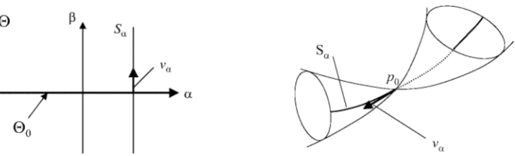
Locally conic models have been introduced by Dacunha-Castelle and Gassiat ([4]) to discuss the uniden- tiÞability. We use their formulation with some mod- iÞcations. Let S = { p(z; θ) | θ ∈ Θ } be a family of probability density functions. We assume that the pa- rameter space Θ is an open subset of A

0

× R , where A

0

is a (d − 1) dimensional space, and write θ = (α, β) according to this decomposition. The model S is called locally conic at p

0

∈ S if the following four conditions are satisÞed;

1. p(z; (α, β)) is diﬀerentiable with respect to β for p

₀

-almost every z.

2. The parameter space Θ contains Θ

0

:= A

0

× { 0 } . 3. The set of parameters to give p

0

is Θ

0

, that is

p(z; (α, β)) = p

0

(z) ⇐⇒ β = 0.

4. For all α ∈ A

0

, the Fisher information of the one- dimensional submodel S

α

= { p(z; α, β) | (α, β ) ∈ Θ } at β = 0 is one; that is, ° °

^∂^log^p(z;α,0)

∂β

° °

L²(p0)

= 1.

If dimA

0

≥ 1, the parameter to give p

0

is uniden- tiÞable. In the set of true parameter Θ

₀

, α can not be identiÞed. Intuitively, the locally conic model is a d-dimensional subset in the space of all the proba- bility density functions, while the point corresponding to p

₀

is a conic singularity in the model (Fig.2). For

each α ∈ A

0

, the one-dimensional submodel S

α

is an identiÞable model, which gives p

0

only by β = 0. A locally conic model is a union of such one-dimensional submodels. The derivative of the log likelihood

v

α

(z) = ∂

∂β log p(z; (α, 0)) (3) can be regarded as a tangent vector along S

α

with unit L

²

(p

0

)-norm. We call the set of such unit tangent vec- tors C = { v

α

| α ∈ A

0

} the basis of the tangent cone, because C deÞnes the tangent cone at the singularity.

3 Likelihood Ratio of a Locally Conic Model

Given an i.i.d. sample Z

1

, . . . , Z

n

following p

0

, the likelihood ratio is deÞned by

L

n

(θ) = X

n

i=1

log p(Z

i

; θ)

p

₀

(Z

_i

) . (4) The MLE ˆ θ is the maximizer of L

n

(θ). We focus on the likelihood ratio of MLE,

sup

θ∈Θ

L

n

(θ), (5)

which essentially expresses the negative training error of a learning machine. In fact, for neural networks with the Gaussian noise model, the likelihood ratio is L

n

(θ) = − 1

2σ

²

X

n

i=1

(y

i

− ϕ(x

i

; θ))

²

+ 1

2σ

²

(y

i

− ϕ

0

(x

i

))

²

. (6) This measures overÞtting of a learning machine. The more a machine Þts with given data, the larger the likelihood ratio is. The likelihood ratio is also used in a statistical test, since, under the regularity conditions of asymptotic theory, we have

2L

n

(ˆ θ) −→ χ

²_d

(n → ∞ ) in law, (7) where χ

²_d

is the chi-square distribution with freedom d. However, if the true parameter is unidentiÞable, the asymptotic distribution of likelihood ratio is not chi-square, or may not be even O

p

(1) as we see later.

Locally conic parameterization is useful for the anal- ysis of the likelihood ratio in unidentiÞable cases. Let β ˆ

α

be MLE in the submodel S

α

. As S

α

is identiÞable, a standard argument using Taylor expansion leads

L

n

(α, β ˆ

α

) = 1

2 U

n

(α)

²

+ o

p

(1) (8) for each Þxed α, where U

n

(α) is deÞned by

U

n

(α) = 1

√ n X

n

i=1

∂ log p(Z

i

; α, 0)

∂β = 1

√ n X

n

i=1

v

α

(Z

i

).

(9)

(3)

Figure 2: Locally conic model: parameter space (left) and the model in the space of density functions (right).

Note that the Fisher information of S

_α

at β = 0 is equal to one by the deÞnition. The likelihood ratio of a locally conic model is, then, given by

sup

θ∈Θ

L

_n

(θ) = sup

α∈A0

L

_n

(α, β ˆ

_α

) = sup

α∈A0

¡1

2 U

_n

(α)

²

+ o

_p

(1) ¢ . (10) The MLE ˆ α, the maximizer of eq.(10), does not nec- essarily converge to a point in A

₀

, but it distributes along Θ

0

.

The random variable U

n

(α) converges in law to the standard normal distribution N (0, 1) for each α. Con- sidering all α, the random element U

n

is a random process over α or the basis of the tangent cone. While the process marginally converges to N(0, 1) for each α, it does not necessarily converge as a random pro- cess. Indeed, the process may not converge uniformly, and the likelihood ratio can diverge to inÞnity. Har- tigan ([9]) shows such divergence in a special case of the normal mixture model with two components. His argument is as follows. The marginal distribution of U

_n

over Þnite points v

_α₁

, . . . , v

_α_m

in the basis of the tangent cone C converges to an m dimensional normal distribution with the covariance E

_p₀

[v

_α_i

v

_α_j

]. If we can Þnd m ”almost uncorrelated” elements in C for arbi- trary m ∈ N , the maximum of the U

n

(α

j

) (1 ≤ j ≤ m) is very close to the maximum of m i.i.d. samples from N (0, 1), which is √

2 log m for large m. As m is arbi- trary, this maximum is not bounded. As an general- ization of this fact we have the following theorem.

Theorem 1. Let S = { p(z; (α, β)) } be locally conic at p

₀

∈ S, and C be its basis of the tangent cone. Assume for each α ∈ A

0

the submodel S

α

= { p(z; α, β) | β } sat- isÞes the regularity conditions of asymptotic normality.

If there is a sequence in C, which converges to zero in p

0

-probability, then, for arbitrary M > 0 we have

n

lim

→∞

Prob ¡ sup

(α,β)

L

n

(α, β) ≤ M ¢

= 0. (11) Proof. See [6].

Eq.(11) shows that L

_n

(ˆ θ) is larger than the constant order O

_p

(1). The above theorem gives a simple suﬃ- cient condition of divergence of the likelihood ratio.

4 Strong OverÞtting of Multilayer Neural Networks

We consider the three-layer perceptron model with H hidden units:

ϕ(x; θ) = X

H

j=1

b

j

s(a

^T_j

x + c

j

) + d, (12) where s(t) = tanh t, and the parameter space is de- noted by Θ

_H

. We assume the output is one-dimensional for simplicity. Suppose that the true function is real- ized by a network with K hidden units

ϕ

₀

(x) = X

K

k=1

b

⁰_k

s(a

⁰_k

x + c

⁰_k

) + d

⁰

, (13) for 0 ≤ K ≤ H. If K ≤ H − 1, the true parameter is unidentiÞable, as we see in Section 1.

We can introduce a locally conic parameterization to formulate this unidentiÞability. A slightly restricted parameter space Θ

^∗_H

is deÞned by Θ

^∗_H

= { θ ∈ Θ

_H

| a

_j

6 = 0, b

_j

6 = 0 (1 ≤ j ≤ H ), (a

_j

, c

_j

) 6 = ± (a

_h

, c

_h

) (1 ≤ j < h ≤ H), (a

_j

, c

_j

) 6 = ± (a

⁰_k

, c

⁰_k

) (1 ≤ k ≤ K, K + 1 ≤ j ≤ H ) } . Note that Θ

^∗_H

eliminates the parameters of functions realizable by a smaller-sized network (see [10]). This reduction does not matter in discussing MLE, since it lies in Θ

^∗_H

with probability one. We introduce a new parameterization by

β = sgn(b

K+1

) q

b

²_K+1

+ · · · + b

²_H

, δ = d − d

⁰

β , ξ

k

= a

_k

− a

⁰_k

β , η

k

= b

_k

− b

⁰_k

β , ζ

k

= c

_k

− c

⁰_k

β , ξ

j

= a

j

, η

j

= b

j

β , ζ

j

= c

j

, (14) for 1 ≤ k ≤ K and K + 1 ≤ j ≤ H. The three-layer perceptron is rewritten using this parameterization:

ψ(x; ω) = X

K

k=1

(b

⁰_k

+ βη

k

) s ¡

(a

⁰_k

+ βξ

k

)x + (c

⁰_k

+ βζ

k

) ¢

+ X

H

j=K+1

βη

j

s(ξ

j

x + ζ

j

) + βδ. (15)

(4)

The new parameter spaces Π

H

and Π

^∗_H

are deÞned by Π

H

= { ω = (ξ

`

, η

`

, ζ

`

, ζ

`

, δ, β) | a

⁰_k

+ βξ

k

6 = 0, b

⁰_k

+ βη

k

6 = 0, (a

⁰_k

+ βξ

k

, c

⁰_k

+ βζ

k

) 6 = ± (a

⁰_h

+ βξ

h

, c

⁰_h

+ βζ

h

), (a

⁰_k

+ βξ

k

, c

⁰_k

+ βζ

k

) 6 = ± (ξ

j

, ζ

j

), (ξ

j

, ζ

j

) 6 =

± (a

⁰_k

, c

⁰_k

), η

j

6 = 0, ξ

j

6 = 0, (ξ

j

, ζ

j

) 6 = ± (ξ

i

, ζ

i

), (1 ≤ k < h ≤ K, K + 1 ≤ j < i ≤ H ), P

H

j=K+1

η

_j²

= 1, η

K+1

> 0, β ∈ R} and Π

^∗_H

= { ω ∈ Π

H

| β 6 = 0 } , respectively. It is easy to see that ϕ(x; θ) = ψ(x; ω) for corresponding θ ∈ Θ

^∗_H

and ω ∈ Π

^∗_H

, and that ψ(x; ω) = ϕ

0

(x) if and only if β = 0. Thus, it suﬃces to consider { ψ(x; ω) | ω ∈ Π

H

} , when MLE is dis- cussed. We deÞne the statistical model of three-layer perceptron S

H

= { p(x, y; ω) | ω ∈ Π

H

} by

p(x, y; ω) = r(y | ψ(x; ω))q(x), (16) for some noise model r(y | s) and input density q(x).

The model S

H

consists of a probability density p

0

(x, y) corresponding to ϕ

0

(x) and densities given by ϕ(x; θ) for θ ∈ Θ

^∗_H

. If we summarize (ξ

1

, . . . , ζ

H

, δ) by α, p(x, y; α, β) gives a locally conic parameterization;

Theorem 2. Under some regularity conditions on r(y | s) and q(x), the multilayer perceptron model S

_H

is locally conic at p

₀

.

Proof. It is easy to see that the conditions 1—3 are sat- isÞed. For the condition 4, taking N (α) =

k

∂β^∂

log p(x, y; (α, 0)) k

L²(p0)

, the parameter ˜ β =

_N^β_(α)

instead of β makes the Fisher information one.

This locally conic model satisÞes the assumptions of Theorem 1, and we have

Theorem 3. Suppose that the model is given by eq.(12) and the true function by eq.(13). If K ≤ H − 1, then, under some regularity conditions on r(y | s) and q(x), we have for arbitrary M > 0

n

lim

→∞

Prob ¡ sup

θ

L

_n

(θ) ≤ M ¢

= 0. (17)

Remark. This theorem means that the likelihood ratio has a larger order than the usual constant order O

p

(1), if a network has redundant hidden unit to realize the target. It indicates very strong overÞtting.

Outline of the proof. We will prove the theorem only for K ≤ H − 2, while it can be proved also for K = H − 1 (see [6]). We have only to consider a submodel g(x, y; ξ, h, t) = r(y | ϕ

0

(x) + βw(x; ξ, h, t))q(x), where w(x; ξ, h, t) is in a function class W = { w(x; ξ, h, t) =

√

1 A(ξ,h,t)

1

2

{ tanh(ξ(x − t+h)) − tanh(ξ(x − t − h)) } . The constant A(ξ, h, t) is a normalization of L

²

norm of the tangent vector v(z; ξ, h, t) deÞned below. Note that the shape of the function w is bell-shaped (Fig.3). For this submodel, the basis of the tangent cone consists of the functions of the form:

v(z; ξ, h, t) = ∂ log r(y | ϕ

0

(x))

∂s w(x; ξ, h, t). (18)

Figure 3: A function in the subclass W (ξ = 10, t = 3, h = 0.5).

We can easily take a sequence (ξ

_n

, h

_n

, t

_n

) such that ξ

_n

→ ∞ , h

_n

→ 0, and v(z; ξ

_n

, h

_n

, t

_n

) converges to zero.

Using the subclass W in the above proof, we can derive also a lower bound of the likelihood ratio, if K ≤ H − 2;

Theorem 4. Suppose that the model is given by eq.(12), and the true function by eq.(13). If K ≤ H − 2, under some regularity conditions on r(y | s) and q(x), there exists δ > 0 such that

lim inf

n→∞

Prob ¡ sup

θ

L

n

(θ) ≥ δ log n ¢

> 0. (19) Outline of the proof. We will show that we can Þnd m = n

^γ

(γ > 0) almost uncorrelated elements in the basis of the tangent cone C for the sample size n. For a closed interval I ⊂ R , we deÞne M (I) =

E

_p₀

£¡

_∂_log_r(y_|_ϕ₀_(x))

∂s

¢

2

χ

_I

(x) ¤

, where χ

_I

(x) is the indica- tor function of I. For m disjoint intervals I

_k

(1 ≤ k ≤ m) in R , we deÞne one-dimensional models r(y | ϕ

₀

(x)+

β √

¹

M(Ik)

χ

_I_k

(x))q(x). The unit tangent vectors at the origin are u

_k

(z) = √

¹

M(Ik)

∂logr(y|ϕ0(x))

∂u

χ

_I_k

(x), which are uncorrelated. Then, under some regularity con- ditions, we can show that the distribution of the m- dimensional random vector V

n

= (

√¹

n

P

n

i=1

u

1

(Z

i

), . . . ,

√¹

n

P

n

i=1

u

m

(Z

i

) ¢

can be approximated by the m- dimensional standard normal distribution for an appro- priate choice of { I

k

} and a suﬃciently small γ. The maximum of | V

n

| is arbitrarily close to √

2 log m =

√ 2γ log n. On the other hand, √

¹

M(I)

χ

I

(x) can be arbitrarily approximated by a function in W , which means there exist n

^γ

functions in W such that eq.(10) has the order of log n. The rigorous proof needs deli- cate discussion. See Fukumizu ([6]) for the details.

The above theorem shows the order of the likeli- hood ratio is at least log n, if the model has two re- dundant hidden units. This order is formerly obtained by Hagiwara et al. ([8]) under stronger assumptions of Gaussian noise and ϕ

₀

(x) ≡ 0.

We can derive an upper bound of the likelihood ra-

tio for wider class of learning machines and the Gaus-

sian noise model.

(5)

Theorem 5. Let F = { ϕ(x; θ) } be a family of func- tions, and ϕ

0

(x) be a bounded function in F . If the VC dimension of F is Þnite, and the noise model is the Gaussian distribution r(y | s) =

√¹

2πσ

exp {−

2σ¹²

(y − s)

²

} , then, we have

sup

θ

L

n

(θ) = O

p

(log n). (20) Outline of the proof. Since the probability of the event { max

1≤i≤n

Y

i

> 2 √

log n } converges to 0, we can con- sider the case in which | Y

i

− ϕ

0

(X

i

) | ≤ 2 √

log n and

| ϕ(x

i

; θ) | ≤ 2 √

log n hold. For a given X = (X

1

, . . . , X

n

), the conditional probability of L

n

(θ) − E

Y

[L

n

(θ) | X ] =

1 σ²

P

n

i=1

(Y

i

− ϕ

0

(X

i

))(ϕ(X

i

; θ) − ϕ

0

(X

i

)) is the nor- mal distribution with mean zero and variance V

_θ,X

= P

n

i=1

(ϕ(X

_i

; θ) − ϕ

₀

(X

_i

))

²

. By the exponential inequal- ity for the tail probability of a normal distribution, for arbitrary λ > 0 we have Prob ¡

L

_n

(θ) ≥ λ −

_2σ¹²

V

_θ,X

| X ¢

≤

√

Vθ,X

√2πλ

e

⁻

λ2

2Vθ,X

. Setting λ = M log n +

_2σ¹2

V

_θ,X

for M > 0, we obtain

Prob ¡

L

_n

(θ) ≥ M log n ¢

≤

^√^σ_2π^√_2M¹_log_n

n

⁻^M/σ²

. (21) Since the VC dimension of F is Þnite, we can Þnd n

^γ

(γ > 0) parameters { θ

k

} such that for arbitrary θ there exists θ

k

satisfying

| L

n

(θ

k

) − L

n

(θ) | ≤ p

2 log n. (22) From eqs.(21) and (22), we obtain the theorem.

From theorems 4 and 5, we see that under the assumptions of Theorem 4 and of additive Gaussian noise, the order of sup

_θ

L

_n

(θ) is exactly log n. In con- trast to the order O

_p

(1) in regular cases, a redundant neural network strongly overÞts with the training data.

5 Regularization in Learning of Multilayer Perceptrons

The very strong overÞtting shown in the previous sec- tion explains the heuristics that regularization is par- ticularly important in neural networks. The proof of the previous theorems suggests that large parameter values in making a delta function can be a cause of the strong overÞtting, which agrees with the Bartlett’s statement ([2]) that large weight values worsen the gen- eralization.

The conventional regularization terms like weight decay are not necessarily reasonable in multilayer neu- ral networks. The weight decay, which adds the term

λ

_n¹₂

k θ k

²

(23) to the loss function, assumes that the `

₂

norm of θ represents the local distance of learning machines. This is not true about a locallcy conic model.

We propose the following regularization method in a locally conic model:

L ˜

n

(α, β) = L(α, β ) − λ

n

Φ(α), Φ(α) = 1

2 k α − α

⁰

k

²

, (24) where α

⁰

is a point in A

0

, and the regularization coef- Þcient λ

n

satisÞes sup

_θ

L

n

(θ) << λ

n

<< √

n. We can see that the maximizer ˜ α of ˜ L

n

converges to α

⁰

in prob- ability. In fact, if k α − α

⁰

k ≥ δ for some δ > 0, the term λ

n

Φ(α) is asymptotically larger than L

n

(α, β), and ˜ L

n

(α, β) becomes negative. Such α cannot be the maximizer, because sup

_β

L ˜

_n

(α

⁰

, β) is asymptotically positive. When we concentrate on a small compact neighborhood K of α

₀

in maximizing ˜ L

_n

(α, β ), we have

sup

α,β

L ˜

n

(α, β) = sup

α∈K

1 2

× n ¡

₁

√n

P

n

i=1

v

α

(X

i

, Y

i

) −

^√^λⁿ_n

(α − α

0

) ¢

2

−

n¹

P

n i=1

∂²logp0(Yi|Xi;α,0)

∂β²

+

^λ_nⁿ

+ o

p

(1) o

.

(25) As the o

_p

(1) term is uniform on the compact set K, from the fact λ

_n

<< √

n, the leading term of the right hand side is sup

_α_∈_K¹₂

¡

₁

√n

P

n

i=1

v

_α

(X

_i

, Y

_i

))

²

, which is of the order O

p

(1). Therefore, the extent of overÞtting is very improved so that the likelihood ratio does not diverge to inÞnity.

In three-layer perceptrons, the locally conic param- eterization depends on the unknown true function. We utilize the parameterization for the constant-zero tar- get ϕ

0

(x) ≡ 0 to construct a regularization term. Tak- ing (η

⁰₁

, . . . , η

_H⁰

) = (

√¹

H

, . . . ,

√¹

H

), ξ

⁰_j

= 1, ζ

_j⁰

= 0, and δ

⁰

= 0 for α

⁰

, the regularization term of the three-layer perceptron is given by

Φ(α)

= 1 2 n

− 1 H (

X

H

j=1

η

j

)

²

+ X

H

j=1

(ξ

j

− 1)

²

+ X

H

j=1

ζ

_j²

+ δ

²

o

= 1 2 n

− ( P

H j=1

b

j

)

²

P

H

j=1

b

²_j

+ X

H

j=1

(a

_j

− 1)

²

+ X

H

j=1

c

²_j

+ d

²

P

j

b

²_j

o

.

(26) From Theorem 4, the coeﬃcient λ

n

is chosen so that log n << λ

n

<< √

n. We use the cosine of the angle

between η and η

0

in regularizing η, since η is restricted

on the unit sphere. A clear diﬀerence from the weight

decay is that Φ(α) does not shrink a

j

and b

j

to zero,

but suppress the large ßuctuation of ˆ α. Also, it is

known ([1]) that in regular cases the best generalization

is attained by the constant order of λ

_n

for weight decay,

while the order of the coeﬃcient λ

_n

for Φ(α) should not

be smaller than log n.

(6)

Average Std. Deviation No regul. 7.06 × 10

⁻⁴

4.51 × 10

⁻⁴

Φ(α) 5.55 × 10

⁻⁴

3.41 × 10

⁻⁴

Weight decay 6.10 × 10

⁻⁴

3.73 × 10

⁻⁴

Table 1: Experimental results on regularization terms.

Average Std. Deviation No regul. 5.33 × 10

⁻⁴

1.18 × 10

⁻⁴

Φ(α) 5.09 × 10

⁻⁴

1.05 × 10

⁻⁴

Weight decay 5.18 × 10

⁻⁴

1.07 × 10

⁻⁴

Table 2: Experimental results on regularization terms in the color conversion problem.

We made two experiments to see the eﬀectiveness of this regularization method. One is an artiÞcial prob- lem, in which the true input-output relation is given by a three-layer perceptron with one hidden unit with additive Gaussian noise, and the model is a three-layer perceptron with four hidden units. The number of training data is 100. We evaluate the mean square error between the true function and trained networks.

Table 1 shows the average and standard deviation over diﬀerent 100 data sets with the same distribution. The second experiment is to learn a color conversion prob- lem. Networks with 10 hidden units are trained to simulate a speciÞc color reproduction system, in which the color ink is supplied by CMY (cyan, magenta, yel- low), but the produced print is measured by the phys- ical color system RGB (red, green, blue). The conver- sion table from RGB to CMY is needed to produce a desired color print ([5]). Instead of measuring a real reproduction system, we prepare 300 data per a sim- ulation by inverting the theoretical Neugebauer equa- tion from CMY to RGB using numerical optimization.

Gaussian noise with variance 0.25 × 10

⁻²

is added to the CMY output as observation noise. Table 2 shows the results over 50 simulations. In both experimetns, the coeﬃcients λ

_n

are decided by preliminary exper- iments. Both of the results show that the proposed regularization method improves the generalization.

6 Discussion

We have analyzed unidentiÞable cases, assuming the true parameter is in the special location. In the case of multilayer networks, this means that the true func- tion is completely realized by a smaller-sized network.

Although one might think this assumption unnatural, we need such analysis to consider the model selection problem. Also, in real world applications of neural net- works, a large number of hidden units are often used, and it is realistic to think there are many almost re-

dundant hidden units in the model. The analysis which assumes the uniqueness of the best parameters does not give a good insight in such situations.

The large order of likelihood ratio is not special to multilayer perceptrons. In many models, such as RBF, normal mixture models, and ARMA, the divergence of the likelihood ratio can be seen. Theorem 1 explains the reason of such divergence in a uniÞed viewpoint.

The analysis of generalization error will be also very important, while we have discussed only training error in this paper. The theoretical analysis of generaliza- tion is very diﬃcult in unidentiÞable cases, because the estimator ˆ β

_α

in a locally conic model does not converge uniformly over α. A new approach would be needed to discuss generalization.

References

[1] S. Amari and N. Murata. Statistical analysis of regu- larization constant - from Bayes, MDL and NIC points of view. In International Work-Conference on ArtiÞ- cial and Natural Neural Networks, 1997.

[2] P. L. Bartlett. For valid generalization, the size of the weights is more important than the size of the network.

In Advances in Neural Information Processing Systems 9, pages 134—140. MIT Press, 1997.

[3] A. M. Chen, H. Lu, and R. Hecht-Nielsen. On the geometry of feedforward neural network error surfaces.

Neural Computation, 5:910—927, 1993.

[4] D. Dacunha-Castelle and E. Gassiat. Testing in lo- cally conic models and application to mixture models.

ESAIM Probability and Statistics, 1:285—317, 1997.

[5] K. Fukumizu. Statistical active learning in multilayer perceptrons. IEEE Transactions on Neural Networks, 11(1):17—26, 2000.

[6] K. Fukumizu. Likelihood ratio of unidentiÞable mod- els and multilayer neural networks. Research Memo- randum 780, The Institute of Statistical Mathematics, 2001.

[7] K. Fukumizu and S. Amari. Local minima and plateaus in hierarchical structures of multilayer per- ceptrons. Neural Networks, 13(3):317—327, 2000.

[8] K. Hagiwara, K. Kuno, and S. Usui. On the prob- lem in model selection of neural network regression in overrealizable scenario. In Proc. of Intern. Joint Conf.

on Neural Networks, volume VI, pages 461—466, 2000.

[9] J. A. Hartigan. A failure of likelihood asymptotics for normal mixtures. In Proceedings of Berkeley Con- ference in Honor of Jerzy Neyman and Jack Kiefer, pages 807—810, 1985.