Quantum gas microscope for ytterbium atoms
Martin Santiago Miranda
A thesis presented for the degree of Doctor of Philosophy
Department of Physics Tokyo Institute of Technology
Japan
In this thesis I report a microscope system for fluorescence imaging of ultra-cold ytterbium atoms trapped in a two-dimensional optical lattice with single-site resolution.
Having a rich variety of isotopes, ytterbium atoms trapped in two-dimensional optical lat- tices are a promising tool to study many-body quantum phenomena resulting from strongly interacting systems. In particular, quantum simulators using fermionic atoms are useful for studying the Fermi-Hubbard model, which is expected to be the key to elucidate the mecha- nism of high temperature superconductors.
In order to observe atoms trapped in an optical lattice, a large number of photons is re- quired to obtain a well resolved image. In contrast with to the conventional method of laser- cooling the atoms while observing their fluorescence, in this experiment a deep potential was created using a combination of a shallow ground-state and a deep excited-state potentials, which confines the heated atoms during the imaging process. The resulting quantum gas mi- croscope was able to resolve individual lattice sites in an optical lattice with a 544 nm spacing.
And I’m not happy with all the analyses that go with just the classical theory, because nature isn’t classical, dammit,
and if you want to make a simulation of nature, you’d better make it quantum mechanical, and by golly it’s a wonderful problem, because it doesn’t look so easy.
Richard Feynman
Contents
1 Introduction 5
1.1 Historical background of laser cooling . . . 5
1.2 Quantum simulation and high temperature superconductors . . . 6
1.3 Purpose of this thesis . . . 7
1.4 Thesis overview . . . 8
1.5 List of publications . . . 9
2 Ytterbium 10 2.1 General properties . . . 10
2.2 Energy structure . . . 11
2.3 Scattering lengths . . . 12
3 Quantum gas microscope 15 3.1 Sub-Doppler cooling methods in alkali atoms . . . 16
3.1.1 Polarization gradient cooling . . . 16
3.1.2 Side-band cooling . . . 17
3.1.3 Sub-doppler cooling in Yb atoms . . . 20
3.2 Simulation . . . 20
3.3 Doppler cooling in ytterbium . . . 22
3.3.1 Magic-wavelength potential and1S0-3P1molasses . . . 22
3.3.2 Estimation of the magic-wavelength for the1S0-3P1transition . . . 25
3.3.3 Deviation from magic-wavelength for the1S0-3P1transition . . . 27
3.3.4 Magic-wavelength potential and1S0-1P1molasses . . . 28
3.3.5 Estimation of the magic-wavelength for the1S0-1P1transition . . . 29
3.4 The deep potential approach . . . 31
3.5 Lifetime and limitations of the deep-potential approach . . . 35
3.5.1 Excitation beam radiative force effects . . . 37
3.6 Solid immersion lens . . . 40
2
4 Experiment: Transport of atoms to the solid immersion lens surface 43
4.1 Introduction . . . 43
4.2 Oven . . . 44
4.3 The vacuum chamber . . . 45
4.4 Laser cooling of Yb atoms . . . 46
4.4.1 Zeeman slower . . . 46
4.4.2 Magneto optical trap . . . 49
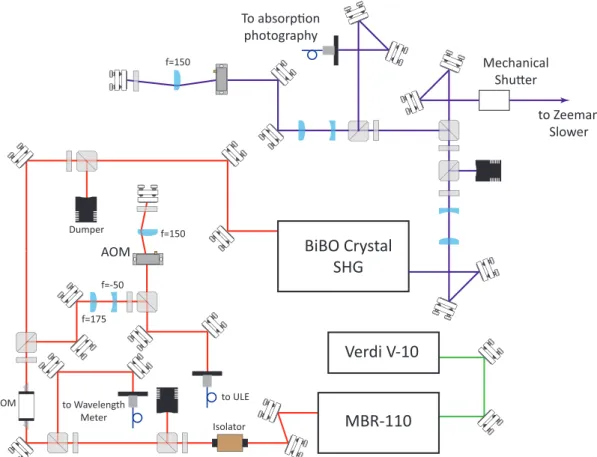
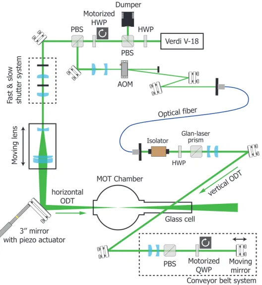
4.5 Transport using optical dipole traps . . . 53
4.5.1 The optical system . . . 53
4.5.2 Horizontal ODT: Loading . . . 53
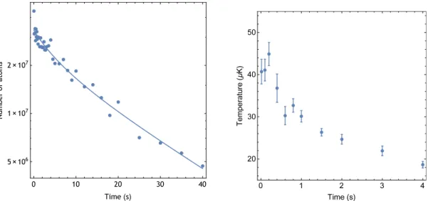
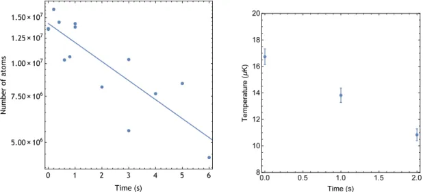
4.5.3 Horizontal ODT: Lifetime and temperature . . . 53
4.5.4 Horizontal ODT: Transport . . . 56
4.5.5 Vertical ODT: Evaporative cooling using a cross ODT . . . 58
4.5.6 Vertical ODT: Transport . . . 61
4.6 Optical accordion . . . 64
4.6.1 System for changing the accordion angle . . . 65
4.6.2 Optical system . . . 67
4.6.3 Accordion lens design . . . 67
4.6.4 Removal of amplified spontaneous emission . . . 69
4.6.5 Alignment of the accordion lens . . . 73
4.6.6 Loading of atoms into the optical accordion . . . 74
4.6.7 Bose-Einstein condensate: Single accordion . . . 75
4.6.8 Bose-Einstein condensate: Double accordion . . . 76
4.6.9 Compression of atoms . . . 77
4.6.10 Density profile of the BEC . . . 80
4.6.11 Stability of the system . . . 82
5 Experiment: Fluorescence imaging 85 5.1 Loading of atoms into the 2D optical lattice . . . 86
5.2 Laser system . . . 87
5.3 Imaging of atoms . . . 88
5.4 Analysis of the microscope performance . . . 90
5.4.1 Microscope resolution . . . 91
5.4.2 Lattice reconstruction . . . 92
5.4.3 Lifetime analysis . . . 94
5.4.4 Fidelity . . . 97
5.5 Light shift in a 5-level diamond system . . . 98
CONTENTS 4
6 Extension to fermionic isotopes 104
6.1 Deep potential . . . 105
6.1.1 AC Stark shift . . . 106
6.1.2 Hyperfine splitting interaction . . . 108
6.1.3 Numerical results . . . 109
6.2 Feasibility of the extension . . . 110
7 Conclusions 112 7.1 Experiment summary . . . 112
7.2 Current quantum gas microscopes . . . 113
7.3 Possible improvements . . . 114
7.4 Tasks . . . 115
7.5 Future experiments . . . 115
A Laser cooling and trapping 116 A.1 Optical dipole trap . . . 116
A.1.1 Optical dipole trap generated by a Gaussian beam . . . 117
A.1.2 Standing Wave . . . 118
A.2 Potential under the solid immersion lens . . . 120
A.3 Evaporative Cooling . . . 123
A.3.1 Efficiency of evaporation . . . 125
A.3.2 Speed of evaporation . . . 125
Introduction
1.1 Historical background of laser cooling
Laser cooling was proposed independently by Hänsch and Schawlow[1]and Wineland and Dehmelt[2]in 1975 and first realized experimentally in 1978 using magnesium ions[3]. The laser cooling techniques were soon extended to neutral atoms in 1981, when an atomic beam of sodium atoms was slowed down to 1.5 K using a resonant laser beam. This was later im- proved in 1982, when the Zeeman slower technique was successfully used to reduce the tem- perature of a sodium atomic beam to less than a few tens of mK[4, 5].
One of the most important applications of laser cooling at that time was the possibility of increasing the accuracy of spectroscopy experiments and atomic clocks, which were mainly limited by Doppler effects and time-dilatation shifts[6]. The current definition of a second is the duration of 9192631770 cycles of radiation corresponding to the transition between the two hyperfine levels of the ground state of the cesium-133 atom. Since the realization of laser cooling, the uncertainty of these cesium atomic clocks improved∼100 times to reach a value of nearly∼3×10⁻¹⁶. That is, the clock will not gain nor lose a second in more than 100 mil- lion years. As big as this number may seem, a new emerging technology called “optical lattice clocks”[7, 8]further improved this number by two orders of magnitude[9, 10]by exploiting optical transitions of ultra-cold neutral atoms, which have frequencies five order of magni- tude larger than hyperfine transitions. Today, laser cooling continues to be a fundamental tool for maintaining frequency standards which support our daily lives through global posi- tioning systems (GPS).
In recent years, laser cooling has also become a state-of-the-art tool to investigate many- body physics in the condensed matter field. When atoms are laser cooled to very low temper- atures, their spatial extent of the wave packet, which is determined by the thermal de Broglie lengthλd B=r
2πħh2
m kBT, increases. When the inter-atomic distance is comparable with the ther- mal de Broglie length, the wave packets of each atom start to overlap and quantum effects
5
CHAPTER 1. INTRODUCTION 6 become important. In the case of bosonic particles, the atomic cloud undergoes a quantum- mechanical phase transition and form a Bose-Einstein condensate (BEC) atn0λ3d B ≈ 2.6, wheren0is the peak atomic number density.
The history of BEC reaches back to 1924, when Satyendra Nath Bose and Albert Einstein predicted the existence of a new state of matter[11, 12]. In 1937, Kaptisa, Allen and Misener reduced the temperature of4He and observed that the liquid helium flowed with no viscosity at temperatures below 2.17 K[13, 14]. One year later, theoretical work by Fritz London showed that the zero viscosity phonema observed in liquid helium was evidence of a new superfluid state of matter, which is intimately related to the BEC of the bosonic4He[15]. The existence and the size of the BEC fraction in superfluid remained controversial for many years, mainly hindered by presence of strong interactions between the atoms in the liquid. In 1968, a∼10%
condensate fraction was observed using neutron scattering techniques[16, 17, 18].
With the aid of laser cooling and evaporative cooling [19]techniques, the first realiza- tion of a “pure” BEC in sodium and rubidium was reported by Nobel prize winners Wieman, Cornell and Ketterle[20, 21]in 1995. In contrast with the BEC of helium where the atoms in the liquid are strongly interacting, the condensates formed with ultra-cold gases allowed researchers to study the properties of weakly interacting systems. In the last 20 years the re- search on BEC has grown explosively, resulting in the observation of many fascinating physics such as condensate interference[22], Anderson localization[23, 24], vortex lattices[25, 26], Berezinskii-Kosterlitz-Thouless transition[27], Feschbach resonances[28, 29], Efimov quan- tum states[30]and the BCS-BEC crossover[31, 32, 33, 34, 35, 36, 37].
1.2 Quantum simulation and high temperature superconductors
Realization of everyday practical applications is one of the major tasks for laser cooled con- densed matter. Ultra-cold atoms trapped in periodical potentials created by light interfer- ence (i.e. optical lattices) demonstrated to be a novel tool for studying interacting many-body quantum systems and creating quantum simulators[38, 39], which serve as a tool to under- stand the physics of solids. Fermionic atoms trapped in optical lattices, in particular, are opti- mal for simulating the Fermi-Hubbard model, which is believed to be the key to elucidate the mechanism of cuprates high temperature superconductors[40, 41, 42, 43, 44]. Understanding such mechanism could lead to the discovery of room-temperature superconductors, produc- ing a huge impact in our daily lives through the improvement on generation and distribution of electric power, transportation (magnetic levitation), medicine (MRI) and the production of faster and more efficient microprocessors.
Why do we need quantum simulators to study cuprate superconductors? Thirty years have passed since Nobel prize winners Bednorz and Muller first discovered cuprate high tem-
perature superconductors in 1986, but the mechanism responsible of generating these ma- terial is still not completely understood. Solid-state physics phenomena resulting in cuprate superconductors is characterized by the movement of electrons inside a crystalline structure.
As the electrons are strongly correlated to each other due to the Coulomb interaction between them, a complete understanding of a single electron state requires the knowledge of the state of all the remaining electrons. In order to simulate strongly correlated quantum system like this using a classical computer, the required number of bits would scale exponentially with the size of the system. Quantum Monte Carlo (QMC) methods, which are effective for solv- ing the Bose-Hubbard Model, notoriously suffer from the so-called “minus sign problem”[45] when solving the Fermi-Hubbard Model. Using ultra-cold neutral atoms trapped in optical lattice can circumvent this problem, as the quantum simulation of the Fermi-Hubbard model can be realized in an experimental way.
In recent years, Markus Greiner team in Harvard University successfully implemented a quantum gas microscope with a resolution of 600 nm capable to address single atoms trapped in a two-dimensional optical lattice[46]. By using a system comprised by a solid immersion lens (SIL) and a high numerical aperture objective lens (NA=0.55), they successfully detected single rubidium atoms in a two-dimensional optical lattice. Later in 2010, Immanuel Bloch team also implemented a high resolution microscope capable of addressing individual Rb atoms using a very high resolution objective lens (NA=0.68)[47]. Several demonstrations of a quantum simulators were realized with the assistance of quantum gas microscopes, includ- ing the simulation of antiferromagnetic spin chains[48], quantum walks[49], and Ising quan- tum magnets[50]. Since the creation of these magnificent tools used to observe and manipu- late rubidium atoms with single-site resolution, the number of researchers trying to develop quantum gas microscopes for other species, which would allow them to simulate a wider di- versity of systems such as strongly correlated Fermi-Hubbard systems, have increased. It was not until 2014 that this technology was successfully extended to ytterbium atoms (this work [51]), and in 2015, to lithium[52, 53, 54], potassium[55, 56, 57]and also ytterbium on a differ- ent way[58].
1.3 Purpose of this thesis
The final objective of our research is to realize the quantum simulation of the Fermi-Hubbard model. One of the biggest challenges to overcome is that the temperature required to reach d-wave superfluidity is below the Neel temperature, which is in the order ofTn/TF ≈0.01, whereTF is the Fermi temperature[59]. Currently, the minimum temperature obtained with fermionic species is in the order ofT/TF ≈0.1, which is one order of magnitude higher than the required temperature. Another difficulty is that temperatures belowT/TF ≈0.1 cannot be
CHAPTER 1. INTRODUCTION 8 measured using the time-of-flight technique[59]. One idea to reduce the temperature of the atoms is to realize spatial filtering[60], which consists in tailor the lattice potential to create high entropy regions than can be later removed. To measure the temperature, instead of mea- suring the momentum distribution using the time-of-flight technique it is possible to obtain the temperature from Quantum Monte Carlo fittings of the in-situ distributions. Both of these techniques, however, require that atoms are resolved with single-site resolution. Although a quantum gas microscope is capable of measuring and the optical lattice with single-site res- olution, when I started my research the technology was only available for rubidium atoms which have only bosonic isotopes.
The purpose of this thesis is to realize a quantum gas microscope of ytterbium atoms, which have a fermionic isotope (173Yb). One of the advantages of Yb is that the ground state is1S0, and thus, there is no electronic spin in the ground state resulting in low decoher- ence times due to magnetic-field fluctuations. Also, the absence of total angular momentum (J =0) results in SU(N) symmetry which prevents spin exchanging collisions. Additionally, Yb have two metastable states with lifetime of several tens of seconds, which are useful for high- resolution spectroscopy[61]and for cooling fermionic atoms in a optical lattice through spa- cial filtering[60]. The3P2state can also be used to to tune inter-atomic interactions through Feshbach resonances[62].
To test the performance of a quantum gas microscope it is convenient to start with the
174Yb bosonic isotope, which have simpler energy structure due to the lack of hyperfine split- ting. The quantum gas microscope presented in this work uses the bosonic isotope, but the same method can be applied to the fermionic isotope without major modifications of the system, as explained in the last chapter.
1.4 Thesis overview
This thesis is organized as follows:
Chapter 2: Ytterbium
A briefly description of the properties of Yb atoms and the most important energy levels.
Chapter 3: Quantum gas microscope
This chapter centers in explaining the requirements of a quantum gas microscope and analyzing the possible fluorescence imaging strategies applicable to Ytterbium atoms.
The “deep potential” strategy used to obtain a large number of photons during imaging is explained in detail, together with simulations to test the feasibility of the method.
Chapter 4: Experiment: Transport of atoms to the SIL surface
To create a two-dimensional optical lattice with trapped Yb atoms, atoms are first re-
quired to be confined in a pancake-shaped region which is thinner than the depth of field of the objective lens. This chapter focuses in the experimental method used to transport ultra-cold Yb atoms under the surface of the solid immersion lens. The “opti- cal accordion” technique used to create a Bose-Einstein condensate and compress the atoms into a thin layer is also explained in detail.
Chapter 5: Experiment: Fluorescence imaging
In this chapter, the experimental method to load the thin condensate of atoms under the surface of the solid immersion lens into a two-dimensional optical lattice is first explained, followed by an analysis of the fluorescence images that were obtained with the quantum gas microscope using the “deep potential” strategy.
Chapter 6: Extension to fermionic isotopes
This chapter focuses in the requirements to extend the quantum gas microscope of yt- terbium atoms to the173Yb fermionic isotope.
1.5 List of publications
The most relevant parts of this thesis have been summarized in the following journal articles:
• M. Miranda, A. Nakamoto, Y. Okuyama, A. Noguchi, M. Ueda, and M. Kozuma, All- optical transport and compression of ytterbium atoms into the surface of a solid immer- sion lens, Physical Review A86, 063615 (2012).
• Martin Miranda, Ryotaro Inoue, Yuki Okuyama, Akimasa Nakamoto, and Mikio Kozuma, Site-resolved imaging of ytterbium atoms in a two-dimensional optical lattice, Physical Review A91, 063414 (2015).
The following journal article is also related to this thesis:
• Toshiyuki Hosoya, Martin Miranda, Ryotaro Inoue, and Mikio Kozuma,Injection locking of a high power ultraviolet laser diode for laser cooling of ytterbium atoms, Review of Scientific Instruments86, 073110 (2015).
Chapter 2
Ytterbium
Ytterbium is a rare earth element and member of the lanthanoid group with atomic number 70 and chemical symbol Yb. With only two electrons in the outermost shell resulting in the absence of electronic spin in the ground state, the Yb atom have a similar energy structure compared with other alkaline-earth-metal-like such as Ca, Sr, and Hg.
2.1 General properties
Naturally occurring ytterbium is composed of seven stable isotopes, five of which are fermions and two are bosons. The natural abundance and nuclear spin of each isotope is summarized in Table 2.1. Compared to other elements, the abundance is more homogeneously distributed between the isotopes.
Mass number Natural abundance Nuclear Spin Type
168 0.13 0 Boson
170 3.05 0 Boson
171 14.3 1/2 Fermion
172 21.9 0 Boson
173 16.12 5/2 Fermion
174 31.8 0 Boson
176 12.7 0 Boson
Table 2.1: Stable isotopes of Yb[63]
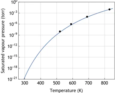
At room temperature, Yb is a solid metal with silvery color, having an atomic mass of 173.04, a density of 6.97 g/cm3, and melting point of 1097 K. Ytterbium is mostly non reac- tive, reacting very slowly to oxygen and water. Due to the high melting point, the saturated vapor pressure at room temperature is very low, thus requiring heating up to 700 K in order to obtain sufficient gas for the experiments.
10
2.2 Energy structure
Ytterbium have two valence electrons in the outermost shell resulting in a1S0ground state with no electronic spin. Similar to other alkaline-earth-metal-like species the excited states are singlet (S=0) or triplet (S=1) states. The energy levels up to 45000 cm−1are summarized in Fig. 2.1. All energy levels were represented by the term symbol2S+1LJ, where S is the total electronic spin (2S+1 is the multiplicity),Lis the total orbital angular momentum of all the electrons in the system (represented by the lettersS,P,D forL=0, . . . , 2), and J is the total angular momentum of the system. The important transitions are briefly described bellow.
1S0↔1P1(399 nm)
An electric dipoled (E1) allowed transition resulting in a strong linewidth of Γ/2π = 27.9 MHz. The strong radiative pressure of this transition is useful for Zeeman slowing of the atomic beam. In this experiment, this transition was used for fluorescence imag- ing the atoms in the two-dimensional optical lattice. Additionally, absorption imaging of the atoms is realized using this transition. This transition is essentially cyclic, with a very small branching ratio of roughly 10−7to the3D1and3D2states[64].
1S0↔3P1(556 nm)
This singlet to triplet transition is prohibited by the LS coupling selection laws. For heavy atoms as Ytterbium, JJ coupling between the orbital and spin motion in the two valence electrons results in the relaxation of the selection law, resulting in this inter- combination transition. With a linewidth ofΓ/2π=181 kHz, this cyclic transition have a low Doppler cooling limit and is ideal for laser cooling in the magneto optical trap.
1S0↔3P0(578 nm)
In this double forbidden transition, the3P0state is very weakly coupled to the1S0ground state with decay rates in the order of tens of millihertz. The resulting ultra-narrow tran- sition is called clock-transition. In contrast with the1S0 ↔3P2 ultra-narrow transi- tion, the absence of electronic angular momentum in the excited state reduces the ef- fects of magnetic fields, making this transition ideal for the creation of a new frequency standard[65, 66]. Additionally, this transition was implemented for the study of two- orbital SU(N) systems[67], and proposed for the implementation in quantum compu- tation[68]and side-band cooling[69].
1S0↔3P2(507 nm)
This quadruple magnetic (M2) transition is also an ultra-narrow transition with a linewidth of a few tens of millihertz. In contrast with the1S0↔3P0clock transition, the excited state have a large magnetic dipole moment of 3µB, which is useful to tune dipole-dipole interactions between atoms in an optical lattice[70]. In recent experiments, the narrow
CHAPTER 2. YTTERBIUM 12 linewidth advantage of this transition was effectively utilized to optical-spectral and magnetic-resonant imaging of atoms trapped in optical lattices[61, 71].
1S0↔3D2(404 nm)
This quadrupole dipole (E2) transition with a linewidth ofΓ/2π=350 kHz is useful to excite atoms to the3P2and3P0states through optical pumping. Atoms excited to the
3D2state decay into the3P1,2states with a ratio of 20:3. As the atoms in the3P1state decay back to the ground state, after a few cycles all the atoms can be pumped into the3P2state[72]. Additionally, by combining the1S0↔3D2transition with the dipole allowed3P2↔3S1transition, it is possible realize optical pumping to the3P0state.
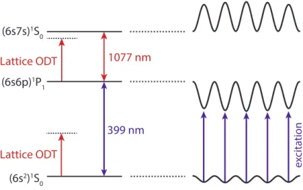
1P1↔(6s7s)1S0(1077 nm)
This dipole allowed transition from the excited1P1have a linewidth ofΓ/2π=3.0 MHz was used in this experiment to produce a deep potential in the excited1P1state. Atoms excited to the(6s7s)1S0state also weakly decay to the3P1state with a decay rate of 2π× 0.2 MHz[73].
2.3 Scattering lengths
The scattering length of each isotope was estimated in previous experiments using two-color photoassociation spectroscopy[74]. The values for the bosonic174Yb isotope and the fermionic isotopes (171Yb and173Yb) were summarized in Table 2.2.
171 173 174
171 -0.15(19) -30.6(3.2) 22.7(7)
173 10.55(11) 7.34(8)
174 5.55(8)
Table 2.2: Calculated s-wave scattering lengths in nm for the171Yb,173Yb and174Yb isotopes [74].
1077 nm
(3.3 MH
z) 611 nm
(210 kH
z) 770
nm (5.9
MH z) 649 nm
(1.5 MH
z)
404 nm (350 kHz)
398.9 nm (27.9 MHz) 555.8 nm (181 kH
z)
578 nm (7 m
Hz)
507 nm(11 mHz)
(6s2) 1S0
(6s6p) 3P0 (6s6p) 3P1 (6s6p) 3P2 (6s6p) 1P1
(5d6s) 3D1 (5d6s) 3D2 (5d6s) 3D3 (6s7p) 3P0
(6s7p) 3P1 (6s7p) 3P2
(5d6s) 1D2 (6s7s) 3S1
(6s7s) 1S0
(6s6d) 3D1 (6s6d) 3D2 (6s6d) 3D3 (6s6d) 1D2 (6s8s) 3S1
(6s8s) 1S0 (6p2) 3P0 (6p2) 3P1 (6p2) 3P2
Ionization Energy (50443.2 cm-1)
532 nm ODT
17288.439 17992.007 19710.388
25068.222
25270.902 38551.93
38174.17 38090.71
24751.948 24489.102 27677.665 40061.51 39966.09 39838.04 39808.72
32694.692 34350.65 41615.04
41939.90 42436.91
43805.42 44760.37
Figure 2.1: Ytterbium energy levels.
CHAPTER 2. YTTERBIUM 14
Atomic Mass Isotope Shift (MHz) Frequency (MHz)
176 -509 751 525 478.5
173(5/2-5/2) -253 751 525 734.3
174 0 751 525 987.7
173(5/2-3/2) 516 751 526 503.7
172 533 751 526 521.1
173(5/2-7/2) 588 751 526 575.7
171(1/2-3/2) 832 751 526 820.2
171(1/2-1/2) 1154 751 527 141.5
170 1192 751 527 180.2
168 1887 751 527 875.2
Table 2.3: Isotope shifts and absolute frequencies of the1S0→1P1transition[75].
Atomic Mass Isotope Shift (MHz) Frequency (MHz) 173(5/2-7/2) -2386.7 539 384 174.1 171(1/2-1/2) -2132.0 539 384 428.8
176 -954.8 539 385 606
174 0 539 386 560.8
172 1000.0 539 387 560.8
170 2286.3 539 388 847.2
173(5/2-5/2) 2311.4 539 382 339.8
168 3655.1 539 380 996.1
171(1/2-3/2) 3804.6 539 380 846.0 173(5/2-3/2) 3805.7 539 380 843.9
Table 2.4: Isotope shifts and absolute frequencies of the1S0→3P1transition[76, 77].
Quantum gas microscope
One site image
1 pixel = 90 nm
1 site = 6x6 pixels
}
Fluorescence from atoms
Excitation light Solid Immersion Lens
emCCD Camera
Eyepiece
High NA objective lens
CCD Camera Image
1000 photons per atom
Figure 3.1: Schematic of a quantum gas microscope. The fluorescence from the atoms trapped in a two-dimensional are captured by a high-numerical-aperture microscope and imaged with a CCD camera.
Quantum gas microscopes are high-resolution fluorescence imaging devices capable of resolving individual atoms trapped in a two-dimensional optical lattice[47, 46]. The con- ventional method to observe atoms trapped in an optical lattice is to excite the atoms and observe the resulting fluorescence using a high-numerical-aperture microscope. Due to the large number of photons required to obtain a well-resolved image, a deep lattice potential is necessary to keep the heated atoms trapped during the imaging process. In the case of ru- bidium atoms, the polarization- gradient-cooling technique[46, 47, 78]worked effectively
15
CHAPTER 3. QUANTUM GAS MICROSCOPE 16 to overcome this difficulty, as it could cool down the atoms to sub-Doppler temperatures while the resultant fluorescence was observed. Unfortunately, this technique is not effective for all the atomic species. In the case of bosonic Yb atoms, for example, the lack of hyper- fine splitting makes impossible the application of sub-Doppler cooling mechanisms such as polarization-gradient-cooling, Raman cooling[79, 80, 81, 56, 52], and electromagnetically in- duced transparency cooling[82, 83, 55].
3.1 Sub-Doppler cooling methods in alkali atoms
In QGM experiments using alkali atoms such as rubidium, lithium and potassium, sub-Doppler techniques are utilized to cool down the atoms while the resultant fluorescence is collected.
Temperatures lower than the Doppler cooling limit resulted in trap lifetimes much larger than the exposure(irradiation) time, which is a required condition to obtain a high fidelity in the fluorescence measurement.
3.1.1 Polarization gradient cooling
In the case of rubidium, the polarization gradient cooling technique was utilized. This tech- nique is schematized in Fig. 3.2. First, two counter-propagating beams having linear polar- ization, which each polarization orthogonal to each other, are used to create a polarization gradient field.
pumping
Figure 3.2: Polarization gradient cooling. Two counter-propagating beams with linear and orthogonal polarization create a polarization gradient field. An atom traveling trough this field is repetitively repumped ’downhill’ resulting in Sisyphus cooling.
To understand why this field is generated, each of the beams can be written as a superpo-
sition ofσ+andσ−polarization beams:
E+= 1 p2
1 1
ei(k x−ωt) , E−= 1 p2
i
−i
ei(−k x−ωt). (3.1)
The interference of this two beams produces two independent standing waves for the circular polarizationsσ+andσ−, having a relative phase ofπ/2:
|E++E−|2∝
sin2(k x−π/4) sin2(k x+π/4)
(3.2)
Next, consider a system having states|↑〉and|↓〉which only couples to theσ−andσ+polar- ization, respectively. Suppose, as in Fig. 3.2 that the atom initially has a state|↑〉where the potential is minimum. As the atom moves climbing the potential wall, the intensity of theσ+ standing wave decreases while the intensity of theσ−one increases. Around the potential maxima, theσ−light repumps the atom to the|↓〉state. In this state, the potential is again a minimum, and the atom will continue moving in the same direction climbing the potential wall, until theσ−standing wave intensity decreases again and the atom is repumped back to the|↑〉state. As the atom repetitiously climb the potential wall, the velocity of the atom can be reduced. This cooling mechanism was named Sisyphus cooling in honor to the king of Ephyra in the Greek mythology, who was punished to roll a heavy ball up to a hill and to throw it back down, repeating this process indefinitely.
The resultant temperature using this cooling method can reach much lower values than the Doppler limit:
T ≈ħhΩ2
8∆ (3.3)
as the temperature can be reduced by increasing the detuning∆of the cooling beams while decreasing their Rabi frequency (laser intensity)Ω2. Using a large detuning∆is also an im- portant feature of this cooling method, as it makes it robust against the inhomogeneities of the light shift in the space produced by the AC Stark shift of the optical lattice. Notice, how- ever, that the trade-off for having low atom temperatures is a reduced photon emission rate, and a lower velocity trap range.
3.1.2 Side-band cooling
Side-band cooling is a technique originally used to cool down ions tightly trapped in a har- monic potential. Consider a two level system with ground stateg
and an excited state|e〉 with a transition frequencyω0. When the oscillator quantum vibrational separationωis suffi-
CHAPTER 3. QUANTUM GAS MICROSCOPE 18 ciently large, the system can be well described by the eigenstatesg,n
,|e,m〉, wherenandm represent the vibrational energy. A laser light with frequencyωL couples each of the ground states
g,n
with the excited states|e,m〉at the transition frequenciesωL =ω0+ (m−n)ω. When the natural linewidth of theg
→ |e〉transitionΓ is sufficiently smaller thanω, it is possible to resolve each of the resonances
g,n
→ |e,m〉in the spectrum. The transition corresponding toωL =ω0where the vibrational energy remains the same (g,n
→ |e,n〉) is called carrier transition, while the transitions to different vibrational energyg,n
→ |e,n〉are denominated side-band transitions.
The side-band cooling technique consists in using a cooling beam that reduces the vi- brational level by 1 in each excitation|e,n〉 →g,n−1
. After the atom is excited, it sponta- neously decay with a high probability to the same vibrational level in the ground state|e,n−1〉 → g,n−1
, completing one cycle and reducing the energy of the atom byħhω. This process is re- peated until the atom is in the motional ground stateg, 0
. The condition that the atom falls with high probability to the same vibrational level in the ground state is satisfied by an atom in the so called Lamb-Dicke regime, where the recoil energy of one photonħhωR is smaller than the quantum vibrational separationħhω. This condition is often written as:
η= sωR
ω =
vt ħh k2
2mω≪1 (3.4)
whereηis the Lamb-Dicke parameter,k is the wavenumber of the cooling light, andmis the mass of the atom.
In the case of40Ca+ions trapped in a Paul trap, the trap frequencies are often in the order ofω/2π≈1 MHz, while the recoil energy of a 729 nm beam is approximatelyωR/2π≈10 kHz, resulting in a Lamb-Dicke parameter ofη≈0.1. The ultra narrow transition at 729 nm have a linewidth of less than 1 Hz, which is enough to resolve the side-band transitions.
Summarizing the above, two conditions are necessary to realize side-band cooling: 1) A cooling laser with a line-width much smaller than the vibrational energy (Γ ≪ω)in order to resolve the side-bands, and 2) A system satisfying the Lamb-Dicke condition, where the recoil energy is much smaller than the vibrational energy (ωR ≪ω).
In the case of neutral atoms trapped in two-dimensional optical lattices, the trap frequen- cies are often in the order ofω/2π≈100 kHz and both conditions become more difficult to be satisfied. For example, the narrow intercombination transition of Ytterbium atoms have a linewidth ofΓ/2π=180 kHz and a recoil energy ofωR/2π=3.7 kHz, resulting inη=0.14 and Γ/ω=1.8. Although the Lamb-Dicke condition is somehow satisfied, the line-width of the cooling laser is too broad to resolve the side-band transitions.
Two different cooling methods can be used to effectively reduce the linewidth of the cool- ing laser, namely, Raman cooling and EIT cooling. Both methods were successfully applied to
cool neutral atoms trapped in two-dimensional optical lattice[79], and also in quantum gas microscopes in recent experiments.
Raman beam
Repump beam
(a) Raman cooling. Two non-resonant beams are used to drive theg1,n
→g2,n−1 Raman transition in a three-level atom. A repump beam is then used to return the atom to theg1,n−1 state, completing one cycle of side-band cool- ing.
coupl ing
laser
coo ling l
aser
Cooling laser absorption spectrum (arb. units)
(b) EIT cooling. A strong coupling laser and a weak cooling laser in aΛ-configuration produce a Fano-like profile in the absorption spectrum (right graph). The detuning and Rabi frequency of each beam can be choosen in such a way that the blue side-band excitation is suppressed, re- sulting in side-band cooling.
Figure 3.3: Two different sub-Doppler cooling methods used to cool down alkali atoms in an optical lattice.
The Raman cooling method consists in using a three-level system to drive a Raman tran- sition, as shown in Fig. 3.3a. A three-level lambda system is usually used for Raman cool- ing, where two of the energy levels (|g1〉and|g2〉) are stable or metastable states, but a ladder system can be also utilized. First, two non-resonant laser beams detuned by∆are used to drive a Raman transition the|g1〉 → |g2〉transition through an intermediate transition|e〉. The linewidth of the Raman transition is given by the formula
Γraman=Ωg e1Ωg e2
∆ (3.5)
whereΩg e1 andΩg e2 are the Rabi frequencies driving the|g1〉 → |e〉and |g2〉 → |e〉tran- sitions, respectively. It is clear in this equation that the linewidth of the Raman transition can be reduced by increasing the detuning∆, which is useful to resolve the side-band transi- tiong1,n
→g2,n−1
necessary for side-band cooling. After the atom is transferred to the g2,n−1
state, a new beam resonant to the|g2〉 → |e〉transition is used to optically pump the atom back to theg1
transition. If the Lamb-Dicke condition is satisfied, the atom will be returned
g1,n−1
to the state, completing one cycle of side-band cooling.
The electromagnetically induced transparency (EIT) cooling utilizes a strong coupling laser detuned by∆rto the|r〉 → |e〉transition to tailor the absorption spectrum of a coupling
CHAPTER 3. QUANTUM GAS MICROSCOPE 20 laser detuned to the|g〉 → |e〉transition (see Fig. 3.3b). The resultant absorption spectrum when∆r>0 is a Fano-like profile having a zero at∆s=∆rcorresponding to the|g,n〉 → |e,n〉 carrier transition. The idea to produce effective side-band cooling is to choose the coupling laser detuning∆r and a Rabi frequencyΩr such that it satisfies the equation:
Γ=
Æ∆r2+Γr2−∆r
2 . (3.6)
In this case, the narrow peak of the Fano-like profile coincides with the red-sideband tran- sition|g,n〉 → |e,n−1〉. This method thus enhances the red side-band transition while it cancels the carrier excitation, which is an ideal condition for side-band cooling.
3.1.3 Sub-doppler cooling in Yb atoms
In the case of the bosonic isotopes of Yb, the lack of hyperfine and magnetic sub-levels in the ground state impedes the use of sub-doppler techniques such as Polarization gradient cooling, Raman cooling and EIT cooling. One idea for realizing sub-doppler cooling is by us- ing two-photon transitions such as the1S0 →3P1→(6s7s)1S0transition having linewidths ofΓ/2π=181 kHz andΓ/2π=210 kHz. Fermionic isotopes have a nuclear spin and conse- quently hyperfine structure in the excited levels. Raman cooling could be possible in principle by using different magnetic sub-levels of the ground state. Also, by using the metastable state
3P2as a cooling basis (which have hyperfine splitting in the fermionic case) it is possible to realize polarization gradient cooling, Raman cooling or EIT cooling.
3.2 Simulation
For the following sections, a computer simulation will be used to test the Doppler cooling and deep potential methods. The simulation realized is semi-classical with the following proper- ties:
Optical lattice The optical potential utilized for the simulations is given by:
V(x,y,z) =V0sin2(kzz)
sin2(kxx) +sin2(kyy)
. (3.7)
wherekx =ky =λlatcosθ2π acc andkz =λlatsinθ2π acc. All simulations were realized for the case θacc =6◦. Note thatV0 is the lattice depth in the x y plane, while the depth in the z direction is 2V0. Due to the geometry of this potential, the hoppings in thez direction will be negligible compared with the ones in thex y plane.
Movement The mechanics of the particle is considered to be classical. For a particle with massmand positionr(t), the differential equation that governs the movement is given
by:
m¨r(t) =F(r,t) (3.8)
where F is the force at the positionrand timet. Using the Euler method, the position of a particle is calculated by the following equations.
r(t˙ +δt) =˙r(t) +F(r,t) m δt r(t +δt) =r(t) +˙r(t)δt
(3.9)
Wannier functions are not considered for the simulation. The initial position and ve- locity of the atom is alwaysr(t) =0 and ˙r(t) =0, respectively.
Photons absorption and emission The probability of absorbing a photon betweent andt+ δt is given by the formula:
p(t) =Γ 2
s0 1+s0+4∆(r)+k·˙r(t)
Γ
2δt (3.10)
wherek·r˙represents the Doppler effect and∆(r)is the detuning of the laser including Stark shift effects at the positionr. In the case of a magic-wavelength, the detuning is homogeneous and∆(r)is constant. When an atom absorbs a photon, the velocity of the particle is immediately increased by ħhkm. Absorption is immediately followed by a photon emission in a random direction.
Population and Rabi oscillations For a multi-level atom, the population in each state|i〉is given byρi i(t,r). The force experienced by the atom is given by:
F(r,t) =−∑
i
ρi i(t,r)∇Vi(r) (3.11)
whereVi(r)is the optical lattice potential on the the state|i〉. Note thatρi i depends on the time, as Rabi oscillations are considered instead of using time averages. For states that are not coupled by a light beam, spontaneus emission rates resulting in transition from a excited state|i〉to a state with a lower energy|j〉are calculated using the formula ρi iΓi j.
Each simulation is stopped when the atom hops to a neighboring site (|kiri(t)|>π2). The lifetime is calculated averaging the obtained photons after 500 repetitions.
CHAPTER 3. QUANTUM GAS MICROSCOPE 22
3.3 Doppler cooling in ytterbium
This section is dedicated to study the possibility of using Doppler cooling to cool down the atoms in the QGM scheme. As the Doppler cooling strongly depends on the detuning of the cooling laser beam∆, it is important to consider the light shift inhomogeneities that arise from having different AC Stark shift in the ground and excited states. The first part of this section is dedicated to study the simplest Doppler cooling setup, where the lattice wavelength λlatis set to the magic-wavelengthλmagicone. In this setup, the wavelength of the lattice ODT is chosen such that the result AC Stark shift in the ground and excited states are exactly the same for every position in space, which produces an homogenous light shift in the space and determines a constant detuning for every point in space∆(x,y,z) =∆(0, 0, 0).
3.3.1 Magic-wavelength potential and1S0-3P1molasses
The1S0-3P1cooling transition in Yb, having a low Doppler cooling limit of 4.4µK, could in principle allow one to obtain long lifetimes even with low potential depths. Simulation results shown in Fig. 3.4a shows the lifetime (in photons) dependency on the potential depth 2V0. For this simulation a six beam molasses setup is used, with each beam having a saturation intensity ofs0=1 and a detuning of∆/Γ=−0.8.
(a) Lifetime dependency on the potential depth 2V0fors0=1 and∆/Γ=−0.8.
(b) Lifetime dependency on the detuning∆for different saturation intensitiess0. The potential depth is fixed at 90µK
Figure 3.4: Lifetimes obtained from the simulation for a magic-wavelength potential using the1S0−3P1transition.
Note that the vertical axis in the figure is in the logarithmic scale. By increasing the poten- tial depth by 30µK the lifetime can be increased one order of magnitude. This is compatible with the Doppler theory, in which atoms have a Gaussian velocity distribution.
To clarify this point, consider the velocity distribution of an atom during Doppler cooling
Figure 3.5: Velocity distribution of an atom during Doppler cooling. The velocity unit is in recoil unitsvR=ħh k/m. The solid line corresponds to a Gaussian fitting.
shown in Fig. 3.5. The profile was obtained from a simple one-dimensional simulation in the free space, for a detuning of∆=−Γ/2 and a saturation intensity ofs0=10−3. The temperature obtained from the width of the Gaussian profile
f1D(v)∝e−m v
2
2kB T (3.12)
resulted inT =4.5µK, which is the Doppler cooling limit. In the three-dimensional case, the lattice depth in thez direction is 2V0while the lattice depth in thex andy directions isV0. Consequently, the atom will mostly escape in thex andy directions and the problem can be considered as two-dimensional. The velocity distribution corresponding to the 2D case is:
f2D(v)∝v e−
m v2
2kB T (3.13)
An atom escapes the lattice site when its kinetic energy is larger than the lattice depthV0. The probability of having an atom with the escape velocity or larger is:
p
v≥
vt2V0 m
=
∫ ∞
v=p
2V0/m
f2D(v)d v∝e−
V0
kB T (3.14)
which decreases exponentially with the potential depth. The lifetime dependency on the laser-cooling detuning∆and saturations0is shown in Fig. 3.4b, where the potential depth was fixed to 2V0=90µK. Fors0=0.1 the optimal saturation was obtained at∆/Γ=−0.6. Note that this result also follows the standard Doppler cooling theory where the Doppler cooling
CHAPTER 3. QUANTUM GAS MICROSCOPE 24 temperature is
kBT =ħhΓ 4
1+s0+ 2Γ∆2 2∆Γ
(3.15) and the Doppler cooling limit is determined by
kBT =ħhΓ 2
p1+s0 when ∆=−Γ 2
p1+s0. (3.16)
For higher laser cooling saturation, the temperature increases and the optimal detuning
∆increases by a ratio ofp
1+s0, which produces a significant reduction in the lifetime. The photon emission rate is also an important factor in the QGC, as the lifetime of the atomic cloud is limited by other factors such as background collisions and lattice light absorptions.
Consequently, a saturation of at leasts0=1 is desired for the experiment. For the following subsections, the analysis will be limited to a saturation ofs0=1.
Six beams 3D molasses Four beams 2D molasses Four beams 3D molasses
Figure 3.6: Three different cooling schemes. (left) 3D molasses cooling using 6 beams in the
±x,±y and±z directions. (center) 2D molasses using 4 beams in the±x and±y directions.
(right) 4 beams in the Brewster angle directions allows cooling in the three dimensions.
(a) 2D molasses using 4 beams in the±xand±y directions.
(b) 4 beams setup as shown in the Fig. 3.6(right) setup.
Figure 3.7: Lifetime as a function of the potential depth 2V0fors0=1 and∆/Γ =−0.8 for two different molasses setup.
Another important point to consider is that in the QGM setup the objective lens is placed
over the solid immersion lens along thez direction (Fig. 3.1). This means that the molasses beams in the+zdirection would enter directly into the camera CCD sensor. One idea to avoid this problem is to use cooling only in the±x and±y directions (Fig. 3.6). Simulation results in Fig. 3.6 shows that, in the case of a 2D cooling, the heating along thez direction causes a significant reduction in the lifetime. In contrast to the potential depth of 2V0=90µK required to obtain a lifetime of 10000 photons in the 3D molasses case, a potential 2V0=450µK would be required to obtain the same lifetime for the 2D molasses approach. Moreover, in this case the lifetime only increases linearly with the potential depth, so a further increment in the life- time would require a very large potential. Another possible idea is to use four cooling beams in the
kˆ1= (cosθB, 0,−sinθB) kˆ2= (−cosθB, 0,−sinθB) kˆ3= (0, cosθB,+sinθB) kˆ4= (0, cosθB, sinθB)
directions, whereθB is the Brewster angle. It can be easily seen that with this setup cooling is possible in all directions. Simulation results in Fig. 3.7b show that this setup produces equal performance as the obtained in the six beams molasses.
3.3.2 Estimation of the magic-wavelength for the1S0-3P1transition
Figure 3.8: Polarizability in the ground1S0state and excited3P1state as a function of the opti- cal dipole trap wavelength. Magic-wavelengths were found 424 nm, 463 nm, 551 nm, 612 nm, 800 nm and 1.53µm.
The magic-wavelength for the1S0-3P1transition is estimated using all the energy levels up to 42000 cm−1. For the calculations, a linear polarized light was used and only them =0 sublevel in both the ground and excited states were considered. In the case of the ground
CHAPTER 3. QUANTUM GAS MICROSCOPE 26
555.
8 nm
1479 nm 1539 nm 458.
457 3 nm .7 nm 611
.3 nm 680.1
nm
(17288.439)
(24489.102) (24751.948) (39808.72) (39838.04)
(32694.69)
(0.00) (34350.65) (41615.04)
42 3.3 n
m
(5d6s) 3D2 (5d6s) 3D1 (6s6d) 3D2 (6s6d) 3D1
(6s6p) 3P1
(6s2) 1S0 (6s7s) 3S1 (6s8s) 3S1
(6s7s) 1S0
From To Wavelength Linewidth Refs.
(6s6p)3P1 (5d6s)3D1 1539 nm 16 kHz [84] (6s6p)3P1 (5d6s)3D2 1479 nm 320 kHz [84]
(6s6p)3P1 (6s7s)3S1 680.1 nm 4.3 MHz [84] (6s6p)3P1 (6s7s)1S0 611.3 nm 210 kHz [85] (6s6p)3P1 (6s6d)3D1 457.7 nm 2.6 MHz [86, 87] (6s6p)3P1 (6s6d)3D2 458.3 nm 2.4 MHz [86, 87] (6s6p)3P1 (6s8s)3S1 423.3 nm 2.7 MHz [86, 87] (6s2)1S0 (6s6p)3P1 555.8 nm 182 kHz
Figure 3.9: Transitions considered for the excited3P1state, and their respective wavelength and line-widths.
state, the1S0-1P1,1S0-3P1and1S0-3D1transitions were used. The transitions from the excited state were summarized in the Fig. 3.9. Although only the transition information for the lower levels is known[84, 85], the lifetime and relative intensities of the upper transitions could be used to roughly estimate the transition linewidths[86, 87]of the remaining transitions.
The calculation results are shown in Fig. 3.8. Six different magic wavelengths with neg- ative polarizability where found, whose wavelengths are 424 nm, 463 nm, 551 nm, 612 nm, 800 nm and 1.53µm. Only the magic-wavelength at 800 nm is far detuned, which makes it a good candidate for creating the two-dimensional optical lattice. Laser sources at 800 nm are also readily available, for example using a Ti:sapphire laser or a tapered amplifier.
3.3.3 Deviation from magic-wavelength for the1S0-3P1transition
What would happen if the lattice wavelength is different from the magic-wavelength one?.
When the atom energy increases due to heating, the atom moves inside the trap, which changes the detuning of the laser cooling and consequently the cooling condition is altered. If the light-shift deviationδdefined by the change of detuning∆(x,y,z)when the atom moves half the lattice spacing
δ=∆(π/2kx, 0, 0)−∆(0, 0, 0) (3.17) is positive, then the detuning absolute value increases when the atom moves[see Fig. 3.10(right)], reducing the efficiency of the Doppler cooling. Similarly, whenδ <0 the detuning absolute value decreases when the atom moves. Eventually, if the deviation is large, the sign of the detuning changes producing heating[see Fig. 3.10(left)].
cooling
heating cooling
cooling
Figure 3.10: (left) If the polarizability in the excited state is lower than the one in the ground state, the detuning of the cooling beams is reduced until eventually heating occurs. (right) A higher polarizability in the excited state do not produce heating, but the efficiency of the Doppler cooling is reduced.
Figure 3.11a shows the simulation results when the lattice wavelength is shifted from the magic wavelength. For the simulation the potential depth was fixed to 2V0/kB =90µK. The asymmetry of the lifetime dependency on the light-shift deviationδis in agreement to the surmise that a negativeδresults in heating and consequently a fast reduction in the lifetime, while a positiveδonly reduces the efficiency of cooling and the lifetime is not greatly affected.
The light-shift deviationδas a function of lattice wavelengthλlatat a fixel potential depth 2V0/kB=90µK is shown in Fig. 3.11b. The3P1-3S1transition at 680 nm causes a rapid incre- ment inδfor wavelengths shorter than the magic wavelength. Forλlat=700 nm the light-shift
CHAPTER 3. QUANTUM GAS MICROSCOPE 28 deviation isδ≈20Γ which reduces the lifetime to∼8000 photons. On the other hand, the change in deviation is smaller (δ≈ −3Γ forλlat=900 nm) but it results in a similar reduction in lifetime.
In conclusion, simulation results shows that it is possible to obtain∼104photons by using a potential depth of 2V0/kB =90µK in a magic-wavelength potential atλlat=800 nm. This potential can be realized using 100 mW of power per beam in the retro-reflected accordion setup, or using 450 mW of power per beam if the standing wave is created by interference of six individual beams. Also, even if the lattice wavelength is deviated by 100 nm from the magic-wavelength, lifetimes of∼8000 photons can be still obtained.
The disadvantages of using this setup is that long exposure times (∼100 ms) would require making the system robust against mechanical vibrations. Also, the maximum power obtain- able at this wavelength is currently limited to 5W using a Ti:sapphire laser pumped by 20 W of light. Additionally, short wavelengths for the lattice result in increased heating due to spon- taneous emission, which is a critical factor to consider when realizing quantum simulations on the Fermi-Hubbard model.
(a) Simulation results of the lifetime depen- dency on light-shift deviationδ.
(b) Light-shift deviationδas a function of lattice wavelengthλlat.
Figure 3.11: Simulation and wavelength calculations for deviations from the magic- wavelength. In both cases the potential depth was fixed to 2V0/kB=90µK.
3.3.4 Magic-wavelength potential and1S0-1P1molasses
Despite the fact that the1S0-1P1transition have a high Doppler cooling limit and, in conse- quence, it is not suitable for cooling, it is interesting to study the lifetime of atoms when this cooling transition is used. Simulation results in Fig. 3.12a shows the lifetime dependency on the potential depth 2V0. For this simulation a six beam molasses setup is used, with each