First principles simulations 第一原理計算

Advanced Laser and Photon Science  レーザー・光量子科学特論 

First principles simulations   第一原理計算

Takeshi Sato 

http://ishiken.free.fr/english/lecture.html  [email protected] 

Interac(on of atoms and molecules with intense electric fields

(10¹³ 〜10¹⁵ W/cm²)

Nuclear aBrac(on & electric field

electron Escape poten(al

barrier

Z

r + E · r

7/5 No. 3

PROGRESS ARTICLE

382 nature physics | VOL 3 | JUNE 2007 | www.nature.com/naturephysics

of the optical pulse controls the kinetic energy², amplitude¹⁷ and phase¹⁸ of the recollision electron and therefore the attosecond pulse¹⁹ that it produces.

In addition to producing attosecond electron and photon pulses, the recollision simultaneously encodes all information on the electron interference. Once the amplitude and phase of the electron interference is encoded in light, powerful optical methods become available to ‘electron interferometry’.

Classical trajectory calculations show that fi ltering a limited band of photon energies near their maximum (cut-off ) confi nes emission to a fraction of a femtosecond¹⁷. Such a burst emerges at each recollision of suffi cient energy. Th e result is a train of attosecond bursts of extreme ultraviolet (XUV) light spaced by T_osc/2 (ref. 1).

For many applications, single attosecond pulses (one burst per laser pulse) are preferred. Th ey emerge naturally from atoms driven by a cosine-shaped laser fi eld comprising merely a few oscillation cycles (few-cycle pulse)³. Th en only the electron pulled back by the central half-wave to its parent ion possesses enough energy to contribute to the fi ltered high-energy emission (Fig. 3). Turning the cosine waveform of the driving laser fi eld into a sinusoidally shaped one (by simply shift ing the carrier wave with respect to the pulse peak⁸) changes attosecond photon emission markedly: instead of a single pulse, two identical bursts are transmitted through the XUV bandpass fi lter. Controlling the waveform of light⁸ has proved critical for controlling electronic motion and photon emission on an attosecond timescale and permitting the reproducible generation of single attosecond pulses¹⁹.

Th e shortest duration of a single attosecond pulse is limited by the bandwidth within which only the most energetic recollision contributes to the emission. In a 5-fs, 750-nm laser pulse this bandwidth relative the emitted energy is about 10%. At photon energies of ~100 eV this translates into a bandwidth of ~10 eV, allowing pulses of about 250 attoseconds in duration¹⁷. At a photon energy of 1 keV (ref. 20) a driver laser fi eld with the above properties will lead to single pulse emission over roughly a 100-eV band, which

may push the frontiers of attosecond technology near the atomic unit of time, 24 attoseconds. Manipulating the polarization state of the driver pulse¹⁷ enables the relative bandwidth of single pulse emission to be broadened^21,22 by ‘switching off ’ recollision before and aft er the main event. Together with dispersion control²³, this technique has recently resulted in near-single-cycle 130-attosecond pulses at photon energies below 40 eV (ref. 24). Confi ning tunnel ionization to a single wave crest at the pulse peak constitutes yet another route to restricting the number of recollisions to one per laser pulse. Superposition of a strong few-cycle near-infrared laser pulse with its (weaker) second harmonic^25,26 is a simple and eff ective way of achieving this goal.

Th is attosecond-pulsed XUV radiation emerges coherently from a large number of atomic dipole emitters. Th e coherence is the result of the atomic dipoles being driven by a (spatially) coherent laser fi eld and the coherent nature of the electronic response of the ionizing atoms discussed above. Th e pulses are highly collimated, laser-like beams, emitted collinearly with the driving laser pulse. Th e next section addresses the concepts that allowed full characterization of the attosecond pulses.

MEASUREMENT TECHNOLOGY

Any pulse measurement method must directly or indirectly compare the phase of diff erent Fourier components of a pulse.

Autocorrelation, SPIDER and FROG, three extensively used methods to characterize optical pulses²⁷, use nonlinear optics to shift the frequency of the Fourier components diff erentially so that neighbouring frequency components can be compared.

Th e electron-optical streak camera — an older ultrafast pulse

Pulse duration (fs)

1970 1980

10^–1 10⁰ 10¹ 10² 10³ 10⁴ 10⁵

1990 Year

2000 2010

Figure 1 Shorter and shorter. The minimum duration of laser pulses fell continually from the discovery of mode-locking in 1964 until 1986 when 6-fs pulses

were generated. Each advance in technology opened new fi elds of science for

measurement. Each advance in science strengthened the motivation for making even shorter laser pulses. However, at 6 fs (three periods of light), a radically different

technology was needed. Its development took 15 years. Now attosecond technology is providing radically new tools for science and is yet again opening new fi elds for real-time measurement. Reprinted in part, with permission from ref. 65.

Ψ_g

Ψ_c = a(k)^eikx–iωt

30 Å

Figure 2 Creating an attosecond pulse. a–d, An intense femtosecond near-infrared or visible (henceforth: optical) pulse (shown in yellow) extracts an electron wavepacket from an atom or molecule. For ionization in such a strong fi eld (a), Newton’s

equations of motion give a relatively good description of the response of the electron.

Initially, the electron is pulled away from the atom (a, b), but after the fi eld reverses, the electron is driven back (c) where it can ‘recollide’ during a small fraction of the laser oscillation cycle (d). The parent ion sees an attosecond electron pulse. This electron can be used directly, or its kinetic energy, amplitude and phase can be

converted to an optical pulse on recollision¹². e, The quantum mechanical perspective.

Ionization splits the wavefunction: one portion remains in the original orbital, the other portion becomes a wave packet moving in the continuum. The laser fi eld moves the wavepacket much as described in a–d, but when it returns the two portions of the wavefunction overlap. The resulting dynamic interference pattern transfers the kinetic energy, amplitude and phase from the recollision electron to the photon.

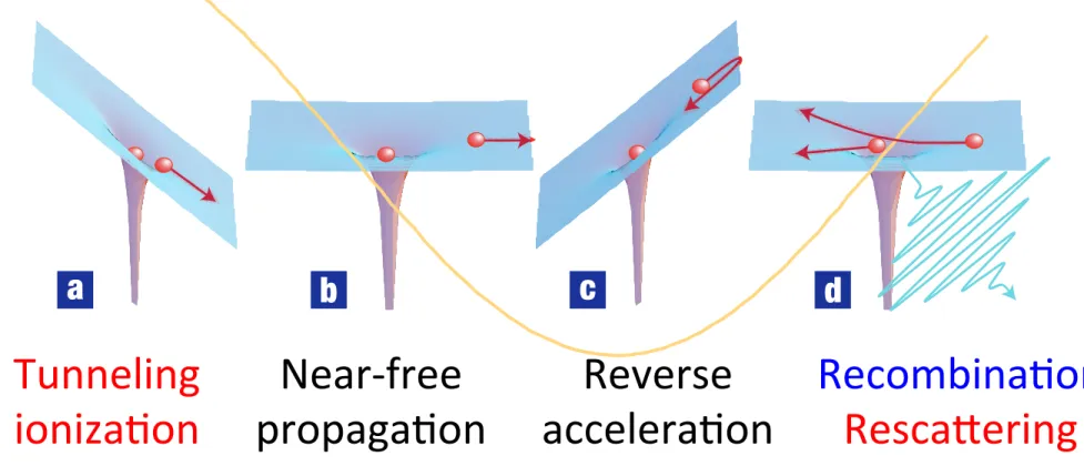
Femtosecond intense laser fields (Visible〜IR, 10¹³ 〜10¹⁵ W/cm²)

Tunneling

ioniza(on Near-free

propaga(on Reverse

accelera(on Recombina(on RescaBering

Corkum, Phys. Rev. LeB. 71, 1994 (1993)

7/5 No. 4

PROGRESS ARTICLE

382 nature physics | VOL 3 | JUNE 2007 | www.nature.com/naturephysics

of the optical pulse controls the kinetic energy², amplitude¹⁷ and phase¹⁸ of the recollision electron and therefore the attosecond pulse¹⁹ that it produces.

In addition to producing attosecond electron and photon pulses, the recollision simultaneously encodes all information on the electron interference. Once the amplitude and phase of the electron interference is encoded in light, powerful optical methods become available to ‘electron interferometry’.

Classical trajectory calculations show that fi ltering a limited band of photon energies near their maximum (cut-off ) confi nes emission to a fraction of a femtosecond¹⁷. Such a burst emerges at each recollision of suffi cient energy. Th e result is a train of attosecond bursts of extreme ultraviolet (XUV) light spaced by T_osc/2 (ref. 1).

For many applications, single attosecond pulses (one burst per laser pulse) are preferred. Th ey emerge naturally from atoms driven by a cosine-shaped laser fi eld comprising merely a few oscillation cycles (few-cycle pulse)³. Th en only the electron pulled back by the central half-wave to its parent ion possesses enough energy to contribute to the fi ltered high-energy emission (Fig. 3). Turning the cosine waveform of the driving laser fi eld into a sinusoidally shaped one (by simply shift ing the carrier wave with respect to the pulse peak⁸) changes attosecond photon emission markedly: instead of a single pulse, two identical bursts are transmitted through the XUV bandpass fi lter. Controlling the waveform of light⁸ has proved critical for controlling electronic motion and photon emission on an attosecond timescale and permitting the reproducible generation of single attosecond pulses¹⁹.

Th e shortest duration of a single attosecond pulse is limited by the bandwidth within which only the most energetic recollision contributes to the emission. In a 5-fs, 750-nm laser pulse this bandwidth relative the emitted energy is about 10%. At photon energies of ~100 eV this translates into a bandwidth of ~10 eV, allowing pulses of about 250 attoseconds in duration¹⁷. At a photon energy of 1 keV (ref. 20) a driver laser fi eld with the above properties will lead to single pulse emission over roughly a 100-eV band, which

may push the frontiers of attosecond technology near the atomic unit of time, 24 attoseconds. Manipulating the polarization state of the driver pulse¹⁷ enables the relative bandwidth of single pulse emission to be broadened^21,22 by ‘switching off ’ recollision before and aft er the main event. Together with dispersion control²³, this technique has recently resulted in near-single-cycle 130-attosecond pulses at photon energies below 40 eV (ref. 24). Confi ning tunnel ionization to a single wave crest at the pulse peak constitutes yet another route to restricting the number of recollisions to one per laser pulse. Superposition of a strong few-cycle near-infrared laser pulse with its (weaker) second harmonic^25,26 is a simple and eff ective way of achieving this goal.

Th is attosecond-pulsed XUV radiation emerges coherently from a large number of atomic dipole emitters. Th e coherence is the result of the atomic dipoles being driven by a (spatially) coherent laser fi eld and the coherent nature of the electronic response of the ionizing atoms discussed above. Th e pulses are highly collimated, laser-like beams, emitted collinearly with the driving laser pulse. Th e next section addresses the concepts that allowed full characterization of the attosecond pulses.

MEASUREMENT TECHNOLOGY

Any pulse measurement method must directly or indirectly compare the phase of diff erent Fourier components of a pulse.

Autocorrelation, SPIDER and FROG, three extensively used methods to characterize optical pulses²⁷, use nonlinear optics to shift the frequency of the Fourier components diff erentially so that neighbouring frequency components can be compared.

Th e electron-optical streak camera — an older ultrafast pulse

Pulse duration (fs)

1970 1980

10^–1 10⁰ 10¹ 10² 10³ 10⁴ 10⁵

1990 Year

2000 2010

Figure 1 Shorter and shorter. The minimum duration of laser pulses fell continually from the discovery of mode-locking in 1964 until 1986 when 6-fs pulses

were generated. Each advance in technology opened new fi elds of science for

measurement. Each advance in science strengthened the motivation for making even shorter laser pulses. However, at 6 fs (three periods of light), a radically different

technology was needed. Its development took 15 years. Now attosecond technology is providing radically new tools for science and is yet again opening new fi elds for real-time measurement. Reprinted in part, with permission from ref. 65.

Ψ_g

Ψ_c = a(k)^eikx–iωt

30 Å

Figure 2 Creating an attosecond pulse. a–d, An intense femtosecond near-infrared or visible (henceforth: optical) pulse (shown in yellow) extracts an electron wavepacket from an atom or molecule. For ionization in such a strong fi eld (a), Newton’s

equations of motion give a relatively good description of the response of the electron.

Initially, the electron is pulled away from the atom (a, b), but after the fi eld reverses, the electron is driven back (c) where it can ‘recollide’ during a small fraction of the laser oscillation cycle (d). The parent ion sees an attosecond electron pulse. This electron can be used directly, or its kinetic energy, amplitude and phase can be

converted to an optical pulse on recollision¹². e, The quantum mechanical perspective.

Ionization splits the wavefunction: one portion remains in the original orbital, the other portion becomes a wave packet moving in the continuum. The laser fi eld moves the wavepacket much as described in a–d, but when it returns the two portions of the wavefunction overlap. The resulting dynamic interference pattern transfers the kinetic energy, amplitude and phase from the recollision electron to the photon.

10^-8 10^-7 10^-6 10^-5 10^-4 10^-3 10^-2 10^-1 10⁰ 10¹ 10²

Intensity (arb. unit)

50 40

30 20

10 0

Harmonic order

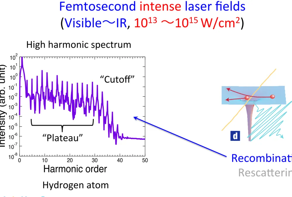
High harmonic spectrum

“Plateau”

“Cutoff”

Hydrogen atom

Femtosecond intense laser fields (Visible〜IR, 10¹³ 〜10¹⁵ W/cm²)

Recombina(on RescaBering

4

10^-8 10^-7 10^-6 10^-5 10^-4 10^-3 10^-2 10^-1 10⁰ 10¹ 10²

Intensity (arb. unit)

50 40

30 20

10 0

Harmonic order

High harmonic spectrum

“Plateau”

Ioniza(on Poten(al (IP) Kine(c energy

@ return (me (K^r)

Cutoff energy

~! = IP + K_r  IP + 3.17U_p Ponderomo(ve energy

U_p = E₀² 4!₀² :

Recombina(on

E(t) = E₀ cos(!₀t) Laser field:

“Cutoff”

Hydrogen atom

Femtosecond intense laser fields (Visible〜IR, 10¹³ 〜10¹⁵ W/cm²)

7/5 No. 6

PROGRESS ARTICLE

382 nature physics | VOL 3 | JUNE 2007 | www.nature.com/naturephysics

of the optical pulse controls the kinetic energy², amplitude¹⁷ and phase¹⁸ of the recollision electron and therefore the attosecond pulse¹⁹ that it produces.

In addition to producing attosecond electron and photon pulses, the recollision simultaneously encodes all information on the electron interference. Once the amplitude and phase of the electron interference is encoded in light, powerful optical methods become available to ‘electron interferometry’.

Classical trajectory calculations show that fi ltering a limited band of photon energies near their maximum (cut-off ) confi nes emission to a fraction of a femtosecond¹⁷. Such a burst emerges at each recollision of suffi cient energy. Th e result is a train of attosecond bursts of extreme ultraviolet (XUV) light spaced by T_osc/2 (ref. 1).

For many applications, single attosecond pulses (one burst per laser pulse) are preferred. Th ey emerge naturally from atoms driven by a cosine-shaped laser fi eld comprising merely a few oscillation cycles (few-cycle pulse)³. Th en only the electron pulled back by the central half-wave to its parent ion possesses enough energy to contribute to the fi ltered high-energy emission (Fig. 3). Turning the cosine waveform of the driving laser fi eld into a sinusoidally shaped one (by simply shift ing the carrier wave with respect to the pulse peak⁸) changes attosecond photon emission markedly: instead of a single pulse, two identical bursts are transmitted through the XUV bandpass fi lter. Controlling the waveform of light⁸ has proved critical for controlling electronic motion and photon emission on an attosecond timescale and permitting the reproducible generation of single attosecond pulses¹⁹.

Th e shortest duration of a single attosecond pulse is limited by the bandwidth within which only the most energetic recollision contributes to the emission. In a 5-fs, 750-nm laser pulse this bandwidth relative the emitted energy is about 10%. At photon energies of ~100 eV this translates into a bandwidth of ~10 eV, allowing pulses of about 250 attoseconds in duration¹⁷. At a photon energy of 1 keV (ref. 20) a driver laser fi eld with the above properties will lead to single pulse emission over roughly a 100-eV band, which

may push the frontiers of attosecond technology near the atomic unit of time, 24 attoseconds. Manipulating the polarization state of the driver pulse¹⁷ enables the relative bandwidth of single pulse emission to be broadened^21,22 by ‘switching off ’ recollision before and aft er the main event. Together with dispersion control²³, this technique has recently resulted in near-single-cycle 130-attosecond pulses at photon energies below 40 eV (ref. 24). Confi ning tunnel ionization to a single wave crest at the pulse peak constitutes yet another route to restricting the number of recollisions to one per laser pulse. Superposition of a strong few-cycle near-infrared laser pulse with its (weaker) second harmonic^25,26 is a simple and eff ective way of achieving this goal.

Th is attosecond-pulsed XUV radiation emerges coherently from a large number of atomic dipole emitters. Th e coherence is the result of the atomic dipoles being driven by a (spatially) coherent laser fi eld and the coherent nature of the electronic response of the ionizing atoms discussed above. Th e pulses are highly collimated, laser-like beams, emitted collinearly with the driving laser pulse. Th e next section addresses the concepts that allowed full characterization of the attosecond pulses.

MEASUREMENT TECHNOLOGY

Any pulse measurement method must directly or indirectly compare the phase of diff erent Fourier components of a pulse.

Autocorrelation, SPIDER and FROG, three extensively used methods to characterize optical pulses²⁷, use nonlinear optics to shift the frequency of the Fourier components diff erentially so that neighbouring frequency components can be compared.

Th e electron-optical streak camera — an older ultrafast pulse

Pulse duration (fs)

1970 1980

10^–1 10⁰ 10¹ 10² 10³ 10⁴ 10⁵

1990 Year

2000 2010

Figure 1 Shorter and shorter. The minimum duration of laser pulses fell continually from the discovery of mode-locking in 1964 until 1986 when 6-fs pulses

were generated. Each advance in technology opened new fi elds of science for

measurement. Each advance in science strengthened the motivation for making even shorter laser pulses. However, at 6 fs (three periods of light), a radically different

technology was needed. Its development took 15 years. Now attosecond technology is providing radically new tools for science and is yet again opening new fi elds for real-time measurement. Reprinted in part, with permission from ref. 65.

Ψ_g

Ψ_c = a(k)^eikx–iωt

30 Å

Figure 2 Creating an attosecond pulse. a–d, An intense femtosecond near-infrared or visible (henceforth: optical) pulse (shown in yellow) extracts an electron wavepacket from an atom or molecule. For ionization in such a strong fi eld (a), Newton’s

equations of motion give a relatively good description of the response of the electron.

Initially, the electron is pulled away from the atom (a, b), but after the fi eld reverses, the electron is driven back (c) where it can ‘recollide’ during a small fraction of the laser oscillation cycle (d). The parent ion sees an attosecond electron pulse. This electron can be used directly, or its kinetic energy, amplitude and phase can be

converted to an optical pulse on recollision¹². e, The quantum mechanical perspective.

Ionization splits the wavefunction: one portion remains in the original orbital, the other portion becomes a wave packet moving in the continuum. The laser fi eld moves the wavepacket much as described in a–d, but when it returns the two portions of the wavefunction overlap. The resulting dynamic interference pattern transfers the kinetic energy, amplitude and phase from the recollision electron to the photon.

Recombina(on RescaBering

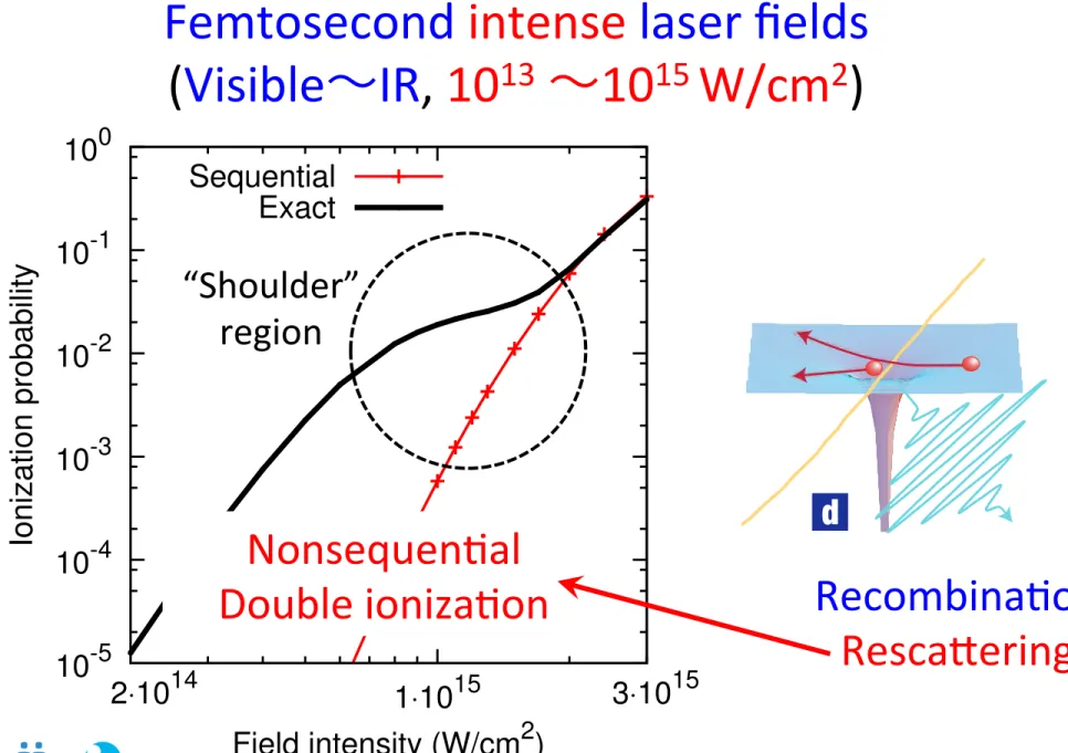
10^-5 10^-4 10^-3 10^-2 10^-1 10⁰

1⋅10¹⁵

Ionization probability

Field intensity (W/cm²)

2⋅10¹⁴ 3⋅10¹⁵

Sequential Exact

Nonsequen(al Double ioniza(on

“Shoulder”

region

Femtosecond intense laser fields (Visible〜IR, 10¹³ 〜10¹⁵ W/cm²)

Time-dependent Schrödinger equa(on

First principles simula(ons

H(t) = XN

i=1

( r²i

2 + XM

A=1

Z_A

|r_i R_A| + V_laser(r_i;t) )

+ XN

i=1

X

j<i

1

|r_i r_j|

i ˙ (r₁, r₂, . . . r_N, t) = H (r₁, r₂, . . . r_N, t)

Computa(onal cost grows factorially w.r.t number of electrons:

Feasible only for H (1 electron), and to a lesser extent He (2 electrons) Time-independent (TID) theories for ground-state: Well established

ü  Density-func(onal theory, Coupled-cluster, Many-body Perturba(on theory…

ü  Atoms, molecules, solids

Time-dependent (TD) theories for non-sta(onary (excited &

con(nuum) states: Far less developed

Single ac(ve electron (SAE) approxima(on Time-dependent Hartree-Fock (TDHF)

Time-dependent density-func(onal theory (TDDFT)

SAE: CANNOT describe

ü  Mul(electron dynamics ü  Mul(channel ioniza(on

i ˙(r) = [h(r) + v_e↵(r)] (r)

v_e↵

TDHF & TDDFT: CANNOT properly describe ü  Tunneling ioniza(on

ü  Electron correla(on

Mul&configura&on Time-Dependent Hartree-Fock (MCTDHF)

1.  Two electron systems (Today)

2.  Second quan&za&on (Today/Next week) 3.  Mul&configura&on &me-dependent

Hartree-Fock method (Next week)

1.  Two electron systems 2.  Second quan&za&on

3.  Mul&configura&on &me-dependent Hartree-Fock method

What is the simplest-possible wavefunction? 

Tunneling ionization 

HF(r₁, r₂) = ₁(r₁) ₁(r₂)

i ₁(r, t) =



h(r, t) + Z

dr₂ | ¹(r₂, t)|²

|r r₂| ¹(r, t) TDHF cannot properly describe TI! 

At least two orbitals are required  

At least two orbitals are required 

Tunneling ionization 

GVB(r₁, r₂) / ¹(r₁) ₂(r₂) + ₂(r₁) ₁(r₂)

GVB(r₁, r₂) / ¹(r₁) ₂(r₂) + ₂(r₁) ₁(r₂)

Generalized Valence Bond (Chemistry)  Extended Hartree-Fock (Physics) 

S₁₂ ⌘ h ¹| ²i 6= 0

Tunneling ionization 

↵₁₂ = h11|12i ES₁₂

↵₂₁ = h22|21i ES₂₁

E = h12|12i + h12|21i S₁₂h22|21i S₂₁h11|12i det(S)

i

 1 S₂₁ S₁₂ 1

 ˙₁

˙₂ =

 h + J₂ + K₂ S₂₁h

S₁₂h h + J₁ + K₁



1

 2

E ↵₂₁ + ES₂₁

↵₂₁ + ES₁₂ E



1 2

Sato and Ishikawa, J. Phys. B 47 (20), 204031 (2014).

H =

X2

i=1

"

1 2

d² dx²_i

p 2

x²_i + 1 + x_iE(t) sin!t

#

+ 1

p(x₁ x₂)² + 1

0.1 0.2 0.3 0.4 0.5 0.6

ψ∗ψ

GVB orbital 1 GVB orbital 2 HF orbital

+2e

Absorber Absorber

Ground-state

-e -e

-0.06 -0.04 -0.02 0.00 0.02 0.04 0.06 0.08 0.10

amplitude / au

2.6 fs

Field

Model simula(on

0.8 PW/cm²

H =

X2

i=1

"

1 2

d² dx²_i

p 2

x²_i + 1 + x_iE(t) sin!t

#

+ 1

p(x₁ x₂)² + 1

Model simula(on

|h (0)| (t)i|^{2 h (t)|(x1+x2)| (t)i}

0.0 0.1 0.2 0.3 0.4 0.5 0.6 0.7 0.8 0.9 1.0

0 1 2 3 4 5 6 7 8

ground state probability

time / optical cycle TDSEHF

GVB

-20 -10 0 10 20 30

0 1 2 3 4 5 6 7 8

dipole moment / au

time / optical cycle TDSEHF

GVB

H =

X2

i=1

"

1 2

d² dx²_i

p 2

x²_i + 1 + x_iE(t) sin!t

#

+ 1

p(x₁ x₂)² + 1

Model simula(on

GVB(r₁, r₂) / ¹(r₁) ₂(r₂) + ₂(r₁) ₁(r₂)

0.00 0.60

-8.0 -4.0 0.0 4.0 8.0

orb. 1

0.00 0.60

-8.0 -4.0 0.0 4.0 8.0

orb. 1 orb. 2

0.00 0.01

-200 -100 0 100 200 t = 1.75T

0.00 0.01

-200 -100 0 100 200 t = 1.75T

0.00 0.01

-200 -100 0 100 200 t = 2.00T

0.00 0.01

-200 -100 0 100 200 t = 2.00T

0.00 0.01

-200 -100 0 100 200 t = 2.25T

0.00 0.01

-200 -100 0 100 200 t = 2.25T

0.00 0.01

-200 -100 0 100 200 t = 2.50T

0.00 0.01

-200 -100 0 100 200 t = 2.50T

0.00 0.01

-200 -100 0 100 200 t = 2.75T

0.00 0.01

-200 -100 0 100 200 t = 2.75T

x (a.u.)

amplitude(a.u.)

TD-GVB  TDHF 

1(t) ₁(t), ₂(t)

-20 0 20 40 60

0 1 2 3 4 5 6

-0.2 -0.1 0.0 0.1 0.2

dipole (a.u.) electric field (a.u.)

time (optical cycle) Field

1

Dipole moment (mean posi(on)

TDHF:

electrons 1 & 2

TD-GVB electron 1

TD-GVB electron 2

At least two orbitals required 

Tunneling ionization 

GVB(r₁, r₂) / ¹(r₁) ₂(r₂) + ₂(r₁) ₁(r₂)

GVB(r₁, r₂) / ¹(r₁) ₂(r₂) + ₂(r₁) ₁(r₂)

Generalized Valence Bond (Chemistry)  Extended Hartree-Fock (Physics) 

S₁₂ ⌘ h ¹| ²i 6= 0

However, non-orthogonal orbitals  result in complicated EOMs 

Orbital redundancy  

+ 

A₁  + A₂ 

1 2 + _{2 1} = C_{1 1 1} + C₃ { ^{1 2} + _{2 1}}

GVB(r₁,r₂) = 1

p2 [ ₁(r₁) ₂(r₂) + ₂(r₁) ₁(r₂)]

= A1 1(r1) 1(r2) + A2 2(r1) 2(r2)

A₁ = 1 + |S₁₂| p2(1 + |S₁₂|²)

S₁₂^⇤

|S₁₂|, A₂ = 1 |S₁₂|

p2(1 + |S₁₂|²)

S₁₂

|S₁₂|,

1 = 1

p2(1 + |S₁₂|)

⇢ S₁₂

|S₁₂| ¹ + ₂

2 = 1

p2(1 + |S |)

⇢ S₁₂^⇤

|S₁₂| ^{2 1}

 Linear transformation of orbitals,  that leaves total wavefunction invariant. 

Orbital redundancy  

close + open 

+  B₁  + B₃  + 

A₁  + A₂  C₁  + C₂  + C₃  + 

close + close  MCTDHF 

Non-orthogonal 

1 2 + _{2 1} = C_{1 1 1} + C₃ { ^{1 2} + _{2 1}}

C_{1 1 1} + C_{2 2 2}, h ¹| ²i = 0 C_{1 1 1} + C_{2 2 2}, h ¹| ²i = 0

C_{1 1 1} + C_{2 2 2}, h ¹| ²i = 0

|h (0)| (t)i|^{2 h (t)|(x1+x2)| (t)i}

0.0 0.1 0.2 0.3 0.4 0.5 0.6 0.7 0.8 0.9 1.0

0 1 2 3 4 5 6 7 8

ground state probability

time / optical cycle TDSEGVB APSG(2)

-20 -10 0 10 20 30

0 1 2 3 4 5 6 7 8

dipole moment / au

time / optical cycle TDSEGVB APSG(2)

(t) = P2

C (t) (1, t) (2, t) / (1, t) (2, t) + (1, t) (2, t)

MCTDHF method for two electron systems 

ü  Propagate both CI coefficients and orbitals  ü  Can improve accuracy by increasing orbitals  

(t) = P2

ij C_ij(t) _i(1, t) _j(2, t) / ¹(1,t) ₂(2, t) + ₂(1, t) ₁(2, t)

= C₁ + C₂ + C₃ + C₄

+ …..

+ C₅ + C₆ (r₁, r₂)

(r₁, r₂, t) =

Xn ij

C_ij(t) _i(r₁, t) _j(r₂, t)

Sequen(al model:

“Shoulder” region:

RescaBering Sequen(al

model:

He à He⁺ à He²⁺

PRL, 78, 1884 (1997)

7/5 No. 25

-3 -2 -1 0 1 2 3

10^-5 10^-4 10^-3 10^-2 10^-1 10⁰

1.0

ionization yield

intensity (10¹⁵ W/cm²)

0.2 3.0

Sequential Exact

Double

ioniza(on yields versus intensity

25

Nonsequen(al double ioniza(on (NSDI)

“Shoulder”

region

Nonsequen(al Sequen(al

Strong Electron correla(on

10^-5 10^-4 10^-3 10^-2 10^-1 10⁰

1.0 × 10¹⁵ Intensity (W/cm²) TDSE

He+

HF: N = 1 GVB: N = 2 N = 4 N = 8 N = 16 N = 28

10^-5 10^-4 10^-3 10^-2 10^-1

10⁰

1.0 × 10¹⁵ Intensity (W/cm²) TDSE

HF: N = 1 EHF: N = 2 N = 4 N = 8

He He

(r₁,r₂,t) =

Xn

C_ij(t) _i(r₁,t) _j(r₂, t)

Summary

ü  At least two non-orthogonal orbitals are required for  describing tunneling ionization  

GVB(r₁, r₂) / ¹(r₁) ₂(r₂) + ₂(r₁) ₁(r₂)

ü  Use of orbital redundancy allows reformulation with  orthonormal orbitals: MCTDHF method 

(r₁, r₂, t) =

Xn

ij

C_ij(t) _i(r₁, t) _j(r₂, t)

i.  Propagate both CI coefficients and orbitals 

ii.  Can be generalized to more-than-two electrons 

1.  Two electron systems (Today)

2.  Second quan&za&on (Today/Next week) 3.  Mul&configura&on &me-dependent

Hartree-Fock method (Next week)

1 2 3 4 5

Mul(configura(on TDHF (MCTDHF) [Kato and Kono, Caillat et al., …]

= C₁ + C₂ + C₃ + C₄ + …..

Superposi(on of ALL Slater determinants within the given number of orbitals

Second quan(za(on

Complete set of one-electron wavefunc(ons (spin-orbitals)

=> Complete set of N-electron Slater determinants

H(t) = XN

i=1

( r²i

2 + XM

A=1

Z_A

|r_i R_A| + V_laser(r_i;t) )

+ XN

i=1

X

j<i

1

|r_i r_j|

i ˙ (r₁, r₂, . . . r_N, t) = H (r₁, r₂, . . . r_N, t)

= XN

i=1

h(r_i, t) + 1 2

XN

i=1

X

j6=i

V (r_i,r_j)

(r₁,r₂, ...r_N, t) = X

I

C_I(t) _I(r₁,r₂, ...r_N)

iC˙_I(t) = X

I⁰

h ^I|H(t)| ^I0iC_I⁰

Z

Second quan(za(on

Second quan(za(on (r₁,r₂, ...r_N, t) = X

I

C_I(t) _I(r₁,r₂, ...r_N)

iC˙_I(t) = X

I⁰

h ^I|H(t)| ^I0iC_I⁰

h ^I|H(t)| ^I0i = Z

⇤I(r1,r2, ...rN)H(r1,r2, ...rN, t) I⁰(r1,r2, ...rN)dr1dr2 · · · drN

| (t)i = X

n

C_n(t)|ni, ^iC˙n(t) = X

m

hn|Hˆ (t)|miC_m

Hˆ(t) = X

µ⌫

h^µ_⌫ (t)ˆa^†_µaˆ_⌫ + 1 2

X

µ⌫

V_⌫^µ aˆ^†_µaˆ^†aˆ ˆa_⌫

n_µ = {0, 1}

|ni = |n₁n₂ · · · n₁i ⌘ Q₁

µ=1(a^†_µ)^nµ|i