R ESEARCH I NSTITUTEFOR M ATHEMATICAL S CIENCESKYOTOUNIVERSITY,Kyoto,Japan ByShinichiMOCHIZUKIApril2015 BOGOMOLOV’SPROOFOFTHEGEOMETRICVERSIONOFTHESZPIROCONJECTUREFROMTHEPOINTOFVIEWOFINTER-UNIVERSALTEICHM¨ULLERTHEORY RIMS-1821

BOGOMOLOV’S PROOF OF THE GEOMETRIC VERSION OF THE SZPIRO CONJECTURE FROM THE POINT OF VIEW OF INTER-UNIVERSAL TEICHM ¨ ULLER THEORY

By

Shinichi MOCHIZUKI

April 2015

R _ESEARCH I NSTITUTE FOR M ATHEMATICAL S _CIENCES

KYOTO UNIVERSITY, Kyoto, Japan

OF THE SZPIRO CONJECTURE FROM THE POINT OF VIEW OF INTER-UNIVERSAL TEICHM ¨ULLER THEORY

Shinichi Mochizuki April 2015

Abstract. The purpose of the present paper is to expose, in substantial detail, certain remarkable similarities between inter-universal Teichm¨uller theory and the theory surrounding Bogomolov’s proofof the geometric version of the Szpiro Conjecture. These similarities are, in some sense, consequences the fact that both theories are closely related to the hyperbolic geometry of the classical upper half-plane. We also discuss various differences between the theories, which are closely related to the conspicuous absence in Bogomolov’s proof of Gaussian distributionsandtheta functions, i.e., which play a central role in inter-universal Teichm¨uller theory.

Contents:

Introduction

§1. The Geometry Surrounding Bogomolov’s Proof

§2. Fundamental Groups in Bogomolov’s Proof

§3. Estimates of Displacements Subject to Indeterminacies

§4. Similarities Between the Two Theories

§5. Differences Between the Two Theories

Introduction

Certain aspects of the inter-universal Teichm¨uller theory developed in [IUTchI], [IUTchII], [IUTchIII], [IUTchIV] — namely,

(IU1) the geometry of Θ^±ellNF-Hodge theaters [cf. [IUTchI], Definition 6.13; [IUTchI], Remark 6.12.3],

(IU2) the preciserelationship betweenarithmetic degrees — i.e., of q-pilot and Θ-pilotobjects — given by the Θ^×μ_LGP-link[cf. [IUTchIII], Definition 3.8, (i), (ii); [IUTchIII], Remark 3.10.1, (ii)], and

(IU3) the estimates of log-volumes of certain subsets of log-shells that give rise to diophantine inequalities [cf. [IUTchIV], §1, §2; [IUTchIII], Re- mark 3.10.1, (iii)] such as the Szpiro Conjecture

— are substantially reminiscent of the theory surrounding Bogomolov’s proof of the geometric version of the Szpiro Conjecture, as discussed in [ABKP],

Typeset byAMS-TEX

1

[Zh]. Put another way, these aspects of inter-universal Teichm¨uller theory may be thought of as arithmetic analogues of the geometric theory surrounding Bo- gomolov’s proof. Alternatively, Bogomolov’s proof may be thought of as a sort of useful elementary guide, orblueprint[perhaps even a sort ofRosetta stone!], for understanding substantial portions of inter-universal Teichm¨uller theory. The author would like to express his gratitude toIvan Fesenkofor bringing to his atten- tion, via numerous discussions in person, e-mails, and skype conversations between December 2014 and January 2015, the possibility of the existence of such fascinating connections between Bogomolov’s proof and inter-universal Teichm¨uller theory.

After reviewing, in§1, §2, §3, the theory surrounding Bogomolov’s proof from a point of view that is somewhat closer to inter-universal Teichm¨uller theory than the point of view of [ABKP], [Zh], we then proceed, in§4, §5, tocompare, by high- lighting varioussimilaritiesanddifferences, Bogomolov’s proof with inter-universal Teichm¨uller theory. In a word, the similarities between the two theories revolve around the relationship of both theories to the classical elementary geometry of the upper half-plane, while the differences between the two theories are closely related to the conspicuous absence in Bogomolov’s proof of Gaussian distri- butions and theta functions, i.e., which play a central role in inter-universal Teichm¨uller theory.

Section 1: The Geometry Surrounding Bogomolov’s Proof

First, we begin by reviewing the geometry surrounding Bogomolov’s proof, albeit from a point of view that is somewhat more abstract and conceptual than that of [ABKP], [Zh].

We denote by M the complex analytic moduli stack of elliptic curves [i.e., one-dimensional complex tori]. Let

M → M

be auniversal coveringof M. Thus, Mis noncanonically isomorphic to the upper half-plane H. In the following, we shall denote by a subscript M the result of restricting to Mobjects over M that are denoted by a subscript M.

Write

ω_M → M

for the [geometric!] line bundle determined by the cotangent space at the origin of the tautological family of elliptic curves over M; ω_M^× ⊆ ω_M for the complement of the zero section in ω_M; EM for the local system over M determined by the first singular cohomology modules with coefficients in Rof the fibers over Mof the tautological family of elliptic curves over M;E_M^× ⊆ EM for the complement of the zero section in EM. Thus, if we think of bundles as geometric spaces/stacks, then there is a natural embedding

ω_M → EM⊗RC

[cf. the inclusion “ω → E” of [IUTchI], Remark 4.3.3, (ii)]. Moreover, this natural embedding, together with the natural symplectic form

- , - E

on EM [i.e., determined by the cup product on the singular cohomology of fibers over M, together with the orientation that arises from the complex holomorphic structure on these fibers], gives rise to a natural metric [cf. the discussion of [IUTchI], Remark 4.3.3, (ii)] on ω_M. Write

(ω_M ⊇ ω^×_M ⊇) ω_M → M

for the S¹-bundle over M determined by the points of ω_M of modulus one with respect to this natural metric.

Next, observe that the natural section ¹₂·tr(−) :C→R[i.e., one-half the trace map of the Galois extension C/R] of the natural inclusion R → C determines a sectionEM⊗RC→ EM of the natural inclusion EM → EM⊗RC whoserestriction to ω_M determines bijections

ω_M → E^∼ M, ω_M^× → E^∼ _M^×

[i.e., of geometric bundles over M]. Thus, at the level of fibers, the bijection ω_M → E^∼ M may be thought of as a [noncanonical] copy of the natural bijection C →^∼ R².

Next, let us write E for the fiber[which is noncanonically isomorphic to R²] of the local system EM relative to some basepoint corresponding to a cusp

“∞”

of M, E_C ^def= E⊗R C, SL(E) for the group of R-linear automorphisms of E that preserve the natural symplectic form - , - ^{E def}= - , - E|^E on E [so SL(E) is noncanonically isomorphic to SL₂(R)]. Now since M is contractible, the local systemsEM, EM^× over Mare trivial. In particular, we obtain natural projection maps

EM E, E^M× E^× E^∠ E^|∠|

— where we write

E^{∠ def}= E^×/R>0

[so E^∠ is noncanonically isomorphic toR^{2∠ def}= R^2×/R^>0 ∼=S¹] and E^∠ E^{|∠| def}= E^∠/{±1}

for the finite ´etale covering of degree 2 determined by forming the quotient by the action of ±1∈SL(E).

Next, let us observe that over each point M, the composite ωM ⊆ ω^×M

→ E∼ M^× E^× E^∠

induces ahomeomorphismbetween the fiber ofωM [over the given point ofM] and E^∠. In particular, for each point ofM, the metric on this fiber of ωM determines a metric on E^∠ [i.e., which depends on the point of M under consideration!]. On

the other hand, one verifies immediately that such metrics on E^∠ always satisfy the following property: Let

D^∠ ⊆ E^∠

be a fundamental domain for the action of ±1 on E^∠, i.e., the closure of some open subset D^∠ ⊆ E^∠ such that D^∠ maps injectively to E^|∠|, while D^∠ maps surjectively to E^|∠|. Thus, ±D^∠ [i.e., the {±1}-orbit of D^∠] is equal to E^∠. Then the volume of D^∠ relative to metrics on E^∠ of the sort just discussed is always equal to π, while the volume of ±D^∠ [i.e., E^∠] relative to such a metric is always equal to 2π.

Over each point ofM, the compositeω^×M

→ E∼ M^× E^×corresponds [noncanon- ically] to a copy of the natural bijection C^{× ∼}→R^2× that arises from thecomplex structureonE determined by the point ofM. Moreover, this assignment of com- plex structures, or, alternatively, points of the one-dimensional complex projective space P(E_C), to points of Mdetermines a natural embedding

M → P(E_C)

[i.e., a copy of the usual embedding of the upper half-plane into the complex pro- jective line], hence also natural actions of SL(E) on Mand EM that are uniquely determinedby the property that they becompatible, relative to this natural embed- ding and the projectionEM E, with the natural actions ofSL(E) onP(E_C) and E. One verifies immediately that these natural actions also determine compatible natural actions of SL(E) on ωM ⊆ ωM^×

→ E∼ M^×, and that the natural action of SL(E) onωM determines a structure of SL(E)-torsoron ωM.

Let SL(E), (ω _M)^∼, (ω^×_M)^∼, (E_M^×)^∼, (E^×)^∼, (E^∠)^∼ be compatible universal coverings of SL(E), ωM, ω^×

M, E^M×, E^×, E^∠, respectively. Thus, SL(E) admits a natural Lie group structure, together with a natural surjection of Lie groups SL(E )SL(E), whose kernel admits anatural generator

τ ∈ Ker(SL(E) SL(E))

determined by the“clockwise orientation”that arises from thecomplex structureon the fibers ofω_M^× overM]. This natural generator determines a natural isomorphism Z →^∼ Ker(SL(E) SL(E)).

Next, observe that the natural actions of SL(E) onωM, ω^×M,EM^×, E^×,E^∠ lift uniquely to compatible natural actions of SL(E) on the respective universal cover- ings (ω_M )^∼, (ω_M^× )^∼, (E_M^×)^∼, (E^×)^∼, (E^∠)^∼. In particular, the natural generator

τ of Z = Ker(SL(E ) SL(E)) determines a natural generator τ^∠ of the group Aut((E^∠)^∼/E^∠) of covering transformations of (E^∠)^∼ E^∠ and hence, taking into account the composite covering (E^∠)^∼ E^∠ E^|∠|, a natural Aut_π(R)- orbit of homeomorphisms [i.e., a “homeomorphism that is well-defined up to composition with an element of Aut_π(R)”]

(E^∠)^{∼ ∼}→ R (Autπ(R))

— where we write Aut_π(R) for the group of self-homeomorphisms R →^∼ R that commutewith translation byπ. Here, the group of covering transformations of the covering (E^∠)^∼ E^∠ is generated by the transformationτ^∠, which corresponds to translationby 2π; the group of covering transformations of the composite covering (E^∠)^∼ E^∠ E^|∠| admits a generator τ^|∠| that satisfies the relation

(τ^|∠|)² = τ^∠ ∈ Aut((E^∠)^∼/E^∠)

and corresponds totranslationbyπ[cf. the transformation “z(−)” of [Zh], Lemma 3.5]. Moreover,τ^|∠| arises from an elementτ^|| ∈SL(E) that lifts−1∈SL(E) and satisfies the relation (τ^||)² =τ. The geometry discussed so far is summarized in the commutative diagram of Fig. 1 below.

SL(E) ( →^∼ R)

(ω_M)^∼ ⊆ (ω_M^× )^∼ →^∼ (E_M^×)^∼ (E^×)^∼ (E^∠)^∼

SL(E)

⏐⏐

⏐⏐ ⏐⏐ ⏐⏐ ⏐⏐ M ←− ω

M ⊆ ω^×

M

→∼ EM^× E^× E^∠

⏐⏐

⏐⏐ ⏐⏐ ⏐⏐ (∼=R^2×) (∼=R^2∠

M ←− ω_M ⊆ ω_M^× →^∼ E_M^× ∼=S¹) Fig. 1: The geometry surrounding Bogomolov’s proof

Section 2: Fundamental Groups in Bogomolov’s Proof

Next, we discuss the various fundamental groups that appear in Bogo- molov’s proof.

Recall that the 12-th tensor powerω_M^⊗12 of the line bundleω_Madmits a natural section, namely, the so-calleddiscriminant modular form, which isnonzeroover M, hence determines a section of ω^×⊗12_M [i.e., the complement of the zero section of ω^⊗12_M ]. Thus, by raising sections of ω_M^× to the 12-th power and then applying thetrivializationdetermined by the discriminant modular form, we obtainnatural holomorphic surjections

ω_M^× ω_M^×⊗12 C^×

— where we note that the first surjection ω_M^× ω^×⊗12_M , as well as the pull-back ωM^× ω^×⊗12M of this surjection to M, is in fact a finite ´etale covering of complex analytic stacks. Thus, the universal covering (ω^×_M)^∼ over ω_M^× may be regarded as a universal covering (ω_M^×⊗12)^{∼ def}= (ω_M^× )^∼ of ω_M^×⊗12. In particular, if we regard Cas a universal covering ofC^× via theexponential mapexp :CC^×, then the surjection ω_M^×⊗12 C^× determined by the discriminant modular form lifts to a surjection

(ω_M^× )^∼ = (ω_M^×⊗12)^∼ C

of universal coverings that is well-defined up to composition with a covering trans- formation of the universal covering exp :CC^×.

Next, let us recall that theR-vector spaceE is equipped with anaturalZ-lattice E_Z ⊆ E

[i.e., determined by the singular cohomology with coefficients in Z]. The set of ele- ments of SL(E) thatstabilize E_Z ⊆E determines a subgroupSL(E_Z)⊆SL(E) [so SL(E_Z) is noncanonically isomorphic toSL₂(Z)], hence also a subgroupSL(E _Z)^def= SL(E )×SL(E)SL(E_Z). Thus, SL(E) ⊇ SL(E_Z) admits a natural action on ω^×M; SL(E )⊇SL(E _Z) admits anatural action on (ω_M^× )^∼. Moreover, one verifies imme- diately that the latter natural action determines a natural isomorphism

SL(E _Z) →^∼ π₁(ω_M^× )

with the group of covering transformations of (ω_M^× )^∼ over ω_M^× , i.e., with the fun- damental group [relative to the basepoint corresponding to the universal covering (ω_M^× )^∼] π₁(ω_M^× ).

In particular, if we use thegenerator−2πi∈Cto identifyπ₁(C^×) withZ, then one verifies easily [by considering the complex elliptic curves that admit automor- phisms of order >2] that we obtain a natural surjective homomorphism

χ : SL(E _Z) = π₁(ω^×_M) π₁(C^×) →^∼ Z

whose restriction to Z →^∼ Ker(SL(E _Z) SL(E_Z)) is the homomorphism Z → Z given by multiplication by 12, i.e.,

χ(τ) = 12, χ(τ^||) = 6 [cf. the final portion of §1].

Finally, we recall that in Bogomolov’s proof, one considers a family of elliptic curves [i.e., one-dimensional complex tori]

X → S (⊆ S)

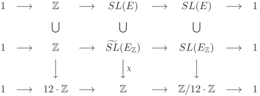
over ahyperbolic Riemann surface S of finite type (g, r) [so 2g−2 +r >0] that has stable bad reduction at every point at infinity [i.e., point ∈S\S] of some compact Riemann surfaceSthatcompactifiesS. Such a family determines aclassifying mor- phism S → M. The above discussion is summarized in the commutative diagrams and exact sequences of Figs. 2 and 3 below.

1 −→ Z −→ SL(E ) −→ SL(E) −→ 1

1 −→ Z −→ SL(E _Z) −→ SL(E_Z) −→ 1

⏐⏐

⏐⏐^χ ⏐⏐

1 −→ 12·Z −→ Z −→ Z/12·Z −→ 1

Fig. 2: Exact sequences related to Bogomolov’s proof

Z = Z →^∼ 12·Z

SL(E) ⊇ SL(E _Z) ^χ Z

⏐⏐

⏐⏐ (ω^×_M)^∼ = (ω_M^×⊗12)^∼ C SL(E) ⊇ SL(E_Z)

⏐⏐

⏐⏐ ⏐⏐^exp ω^×M ω^×⊗12M C^×

⏐⏐

⏐⏐

X −→ S −→ M ←− ω^×_M ω^×⊗12_M C^×

Fig. 3: Fundamental groups related to Bogomolov’s proof

Section 3: Estimates of Displacements Subject to Indeterminacies

We conclude our review of Bogomolov’s proof by briefly recalling the key points of the argument applied in this proof. These key points revolve around estimates of displacements that are subject to certain indeterminacies.

Write

Aut_π(R≥0)

for the group of self-homeomorphisms R≥0 →∼ R≥0 that stabilizeandrestrict to the identity on the subset π·N⊆R≥0 and R_|π| for the set of Aut_π(R≥0)-orbits of R≥0

[relative to the natural action of Aut_π(R≥0) on R≥0]. Thus, one verifies easily that R|π| =

n∈N

{ [n·π] }

∪

m∈N

{ [(m·π,(m+ 1)·π)] }

— where we use the notation “[−]” to denote the element in R_|π| determined by an element or nonempty subset of R≥0 that lies in a single Aut_π(R≥0)-orbit. In particular, we observe that the natural order relation on R≥0 induces a natural order relation onR|π|.

For ζ∈SL(E ), write

δ(ζ) ^def= { [ |ζ(e) −e| ] | e∈(E^∠)^∼ } ⊆ R_|π|

— where the“absolute value of differences of elements of(E^∠)^∼”is computed with respect to some fixed choice of a homeomorphism (E^∠)^{∼ ∼}→ R that belongs to the natural Autπ(R)-orbit of homeomorphisms discussed in §1, and we observe that it follows immediately from the definition of R_|π| that the subset δ(ζ) ⊆ R_|π| is in fact independent of this fixed choice of homeomorphism.

Since [one verifies easily, from the connectednessof the Lie group SL(E), that]

τ^|| belongs to the center of the group SL(E ), it follows immediately [from the

definition of R|π|, by considering translates of e ∈ (E^∠)^∼ by iterates of τ^||] that the set δ(ζ) is finite, hence admits amaximal element

δ^sup(ζ) ^def= sup(δ(ζ))

[cf. the “length” (−) of the discussion preceding [Zh], Lemma 3.7]. Thus, δ((τ^||)ⁿ) = { [ |n| ·π ] }, δ^sup((τ^||)ⁿ) = [ |n| ·π ]

for n ∈ Z [cf. the discussion preceding [Zh], Lemma 3.7]. We shall say that ζ∈SL(E ) isminimal if δ^sup(ζ) determines a minimal element of the set{δ^sup(ζ· (τ)ⁿ)}ⁿ∈Z.

Next, observe that thecusp“∞” discussed in§1 may be thought of as achoice of some rank one submoduleE_∞ ⊆E_Z for which there exists a rank one submodule E₀ ⊆ E_Z — which may be thought of as a cusp “0” — such that the resulting natural inclusions determine an isomorphism

E_∞⊕E₀ →^∼ E_Z

ofZ-modules. Note that sinceE_∞ andE₀ arefreeZ-modules of rank one, it follows [from the fact that the automorphism group of the group Z is of order two!] that there exist natural isomorphismsE_∞^⊗2 →^∼ E₀^⊗2 →^∼ Z. On the other hand, thenatural symplectic form - , - E_Z def

= - , - E|E_Z on E_Z determines an isomorphism of E_∞ with thedual of E₀, hence [by applying the natural isomorphism E₀^⊗2 →^∼ Z] a natural isomorphism E_∞ →^∼ E₀.

This natural isomorphism E_∞ →^∼ E₀ determines a nontrivial unipotent auto- morphism τ_∞ ∈SL(E_Z) of E_Z = E_∞⊕E₀ that fixes E_∞ ⊆E_Z — i.e., which may be thought of, relative to natural isomorphismE_∞ →^∼ E₀, as the matrix _{1 1}

0 1

— as well as an SL(E_Z)-conjugate unipotent automorphism τ₀ ∈ SL(E_Z) — i.e., which may be thought of, relative to natural isomorphismE_∞→^∼ E₀, as the matrix _{1 0}

−1 1

. Thus, the product

τ_∞·τ₀ = 1 1

0 1

·

1 0

−1 1

=

0 1

−1 1

∈ SL(E_Z)

lifts, relative to a suitable homeomorphism (E^∠)^{∼ ∼}→ Rthat belongs to thenatural Autπ(R)-orbit of homeomorphismsdiscussed in§1, to an elementτθ ∈SL(E _Z) that induces the automorphism of R given by translation by θ for some θ ∈ R such that |θ|= ¹₃π.

The key observations that underlie Bogomolov’s proof may be summarized as follows [cf. [Zh], Lemmas 3.6 and 3.7]:

(B1) Every unipotent element τ ∈SL(E) lifts uniquely to an element

τ ∈ SL(E)

thatstabilizesandrestricts to the identityon some (τ^|∠|)^Z-orbitof (E^∠)^∼. Such a τis minimal and satisfies

δ^sup(τ) < [π].

(B2) Every commutator [α, β] ∈SL(E) of elements α, β∈SL(E ) satisfies δ^sup([α, β]) < [2π].

(B3) Let τ_∞,τ₀ ∈SL(E _Z) be liftings of τ_∞, τ₀ ∈SL(E_Z) as in (B1). Then

τ_∞ ·τ₀ =τθ, and θ = ¹₃π >0.

In particular,

(τ_∞·τ₀)³ =τ^||, χ(τ_∞) =χ(τ₀) = 1, χ(τ) = 2·χ(τ^||) = 12.

Observation (B1) follows immediately, in light of the various definitions in- volved, together with the fact that τ^|| belongs to the center of the group SL(E ), from the factτ fixesthe [distinct!] images inE^∠ of±v ∈E for somenonzerov∈E. Next, let us write |SL(E)|^def= SL(E)/{±1}. Then observe that since the gen- erator τ^|| of Ker(SL(E ) SL(E) |SL(E)|) belongs to the center of SL(E ), it follows that every commutator [α, β] as in observation (B2) is completely deter- mined by the respective images |α|,|β| ∈ |SL(E)| of α, β∈SL(E ). Now recall [cf.

the proof of [Zh], Lemma 3.5] that it follows immediately from anelementary linear algebra argument — i.e., consideration of a solution “x” to the equation

det_{a b}

c d

−_{1 x}

0 1

= 0

associated to an element _{a b}

c d

∈ SL₂(R) such that c = 0 — that every element of SL(E) other than −1 ∈ SL(E) may be written as a product of two unipotent elements of SL(E). In particular, we conclude that every commutator [α, β] = (α·β·α⁻¹)·β⁻¹ as in observation (B2) may be written as aproduct

τ₁·τ₂·τ₂^∗·τ₁^∗

of four minimal liftings “τ” as in (B1) such that τ₁^∗, τ₂^∗ are SL(E)-conjugate to

τ₁⁻¹, τ₂⁻¹, respectively. On the other hand, it follows immediately from the fact that the action on E^∠ of any nontrivial [i.e., = 1] unipotent element of SL(E) has precisely two fixed points [i.e., precisely one {±1}-orbit of fixed points] that, for i = 1,2, there exists an element i ∈ {±1} such that, relative to the action of SL(E ) on (E^∠)^{∼ ∼}→R,τ_iⁱ maps every elementx∈Rto an elementRτ_iⁱ(x)≥x.

[Indeed, consider thecontinuityproperties of the mapRx→τi(x)−x∈R, which is invariant with respect to translation by π in its domain!] Moreover, since any element ofSL(E ) induces a self-homeomorphism of (E^∠)^{∼ ∼}→Rthatcommuteswith the action of τ^||, hence is necessarily strictly monotone increasing, we conclude that, for i= 1,2, (τ_i^∗)ⁱ maps every element x∈Rto an elementR(τ_i^∗)ⁱ(x)≤x.

In particular, any computation of the displacements∈Rthat occur as the result of applying the above product τ₁·τ₂ ·τ₂^∗·τ₁^∗ to some element of (E^∠)^{∼ ∼}→ R yields, in light of the estimates δ^sup(τ₁)<[π], δ^sup(τ₂)<[π] of (B1), a sum

(((a^∗₁+a^∗₂) +a₂) +a₁) = (a₁+a^∗₁) + (a₂+a^∗₂) ∈ R for suitable elements

a₁ ∈ ₁·[0, π) ⊆ R; a^∗₁ ∈ −₁·[0, π) ⊆ R; a₂ ∈ ₂·[0, π) ⊆ R; a^∗₂ ∈ −₂·[0, π) ⊆ R.

Thus, the estimateδ^sup([α, β]) <[2π] of observation (B2) follows immediately from the estimates |a₁+a^∗₁|< π, |a₂+a^∗₂|< π.

Next, observe that sinceπ <2π−¹₃π, it follows immediately that{[0],[(0, π)]} ∩ δ(τ_θ·(τ)ⁿ) = ∅ for n= 0. On the other hand, (B1) implies that [0]∈δ(τ₀) and δ^sup(τ_∞) < π, and hence that {[0],[(0, π)]} ∩ δ(τ_∞ ·τ₀) = ∅. Thus, the relation

τ_∞ · τ₀ = τ_θ of observation (B3) follows immediately; the positivity of θ follows immediately from the clockwisenature [cf. the definition “τ” in the final portion of §1] of the assignments ₁

0

→ ₀

−1

, ₀

1

→₁

1

determined by τ_∞·τ₀.

Next, recall the well-knownpresentationvia generatorsα^S₁, . . . , α_g^S,β₁^S, . . . , β_g^S, γ₁^S, . . . , γ_r^S [where γ₁^S, . . . , γ_r^S generate the respective inertia groups at the points at infinity S \S of S] subject to the relation

[α₁^S, β₁^S]·. . .·[α^S_g, β_g^S]·γ₁^S·. . .·γ_r^S = 1

of the fundamental group ΠS of the Riemann surfaceS. These generators map, via the outer homomorphism Π_S → Π_M induced by the classifying morphism of the family of elliptic curves under consideration, to elements α₁, . . . , αg, β₁, . . . , βg, γ₁, . . . , γ_r subject to the relation

[α₁, β₁]·. . .·[αg, βg]·γ₁·. . .·γr = 1

of the fundamental group Π_M =SL(E_Z) [for a suitable choice of basepoint] ofM. Next, let us choose liftings α₁, . . . ,αg, β₁, . . . ,βg, γ₁, . . . ,γr of α₁, . . . , αg, β₁, . . . , βg, γ₁, . . . , γr to elements of SL(E _Z) such that γ₁, . . . ,γr are minimal liftings as in (B1). Thus, we obtain a relation

[α₁,β₁]·. . .·[α_g,β_g]·γ₁·. . .·γ_r = (τ)ⁿ = (τ^||)²ⁿ

in SL(E _Z) for some n ∈ Z. The situation under consideration is summarized in Fig. 4 below.

Π_S −→ Π_M

SL(E) ⊇ SL(E _Z) SL(E_Z) ⊆ SL(E)

(E^∠)^∼ E^∠

Fig. 4: The set-up of Bogomolov’s proof

Now it follows from the various definitions involved, together with the well- known theory of Tate curves, that, for i= 1, . . . , r,

the element γi is an SL(E_Z)-conjugate of τ_∞^vi

for some v_i ∈N. Put another way,v_i is theorder of the “q-parameter” of the Tate curvedetermined by the given family X →S at the point at infinity corresponding to γ_i^S.

Thus, by applying χ(−) to the above relation, we conclude [cf. the discussion preceding [Zh], Lemma 3.7] from theequalities in the final portion of (B3) [together with the evident fact that commutatorsnecessarily lie in the kernel of χ(−)] that

(B4) The “orders of q-parameters” v₁, . . . , v_r satisfy the equality r

i=1

v_i = 12n

— where n ∈Z is the quantity defined in the above discussion.

On the other hand, by applying δ^sup(−) to the aboverelation, we conclude [cf.

the discussion following the proof of [Zh], Lemma 3.7] from the estimates of (B1) and (B2), theequalityof (B4), and the equalityδ^sup((τ^||)ⁿ) = [|n|·π ], forn∈Z,

that ^r

i=1

π

+ ^g

j=1

2π

> 2π·n = ¹₆ ·π· r i=1

vi

— i.e., that

(B5) The “orders of q-parameters” v₁, . . . , v_r satisfy the estimate

1 6 · ^r

i=1

v_i < 2g+r

— where (g, r) is the type of the hyperbolic Riemann surface S.

Finally, we conclude [cf. the discussion following the proof of [Zh], Lemma 3.7] the geometric version of the Szpiro inequality

1 6 · ^r

i=1

vi ≤ 2g−2 +r

by applying (B5) [multiplied by a normalization factor ¹_d] to the families obtained from the given family X → S by base-changing to finite ´etale Galois coverings of S of degree d and passing to the limitd → ∞.

Section 4: Similarities Between the Two Theories

We are now in a position toreap the benefits of the formulation of Bogomolov’s proof given above, which is much closer “culturally” to inter-universal Teichm¨uller theory than the formulation of [ABKP], [Zh].

We begin by considering the relationship between Bogomolov’s proof and (IU1), i.e., the theory of Θ^±ellNF-Hodge theaters, as developed in [IUTchI].

First of all, Bogomolov’s proof clearly centers around the hyperbolic geometry of theupper half-plane. This aspect of Bogomolov’s proof is directly reminiscent of the detailed analogy discussed in [IUTchI], Remark 6.12.3; [IUTchI], Fig. 6.4, between the structure of Θ^±ellNF-Hodge theaters and the classical geometry of the upper half-plane. In particular, one may think of

the additive F^±l -symmetry portion of a Θ^±ellNF-Hodge theater as corresponding to the unipotent transformations τ_∞, τ₀, γ_i

that appear in Bogomolov’s proof and of

the multiplicative F_l -symmetry portion of a Θ^±ellNF-Hodge theater as corresponding to the toral/“typically non-unipotent” transforma- tions τ_∞·τ₀, αi, βi

that appear in Bogomolov’s proof, i.e., typically as products of two non-commuting unipotent transformations [cf. the proof of (B2)!].

One central aspect of the theory of Θ^±ellNF-Hodge theaters developed in [IUTchI] lies in the goal of somehow“simulating”a situation in which the module of l-torsion points of the given elliptic curve over a number field admits a “global multiplicative subspace” [cf. the discussion of [IUTchI], §I1; [IUTchI], Remark 4.3.1]. One way to understand this sort of “simulated” situation is in terms of the one-dimensional additive geometry associated to a nontrivial unipotent transformation. That is to say, whereas, from an a priori point of view, the one- dimensional additive geometries associated to conjugate, non-commuting unipotent transformations aredistinctandincompatible, the “simulation” under consider- ation may be understood as consisting of the establishment of some sort ofgeom- etryin which these distinct, incompatible one-dimensional additive geometries are somehow “identified” with one another as a single, unified one-dimensional additive geometry. This fundamental aspect of the theory of Θ^±ellNF-Hodge theaters in [IUTchI] is thus reminiscent of the

single, unified one-dimensional objects E^∠ ( →^∼ S¹), (E^∠)^∼( →^∼ R) in Bogomolov’s proof which admit natural actions by conjugate, non-commuting unipotent transformations ∈SL(E) [i.e., such asτ_∞, τ₀] and their minimal liftings to SL(E) [i.e., such as τ_∞, τ₀ — cf. (B1)].

The issue of simulation of a “global multiplicative subspace” as discussed in [IUTchI], Remark 4.3.1, is closely related to the application ofabsolute anabelian geometryas developed in [AbsTopIII], i.e., to the issue of establishing global arith- metic analogues for number fields of the classical theories of analytic continua- tion and K¨ahler metrics, constructed via the use of logarithms, on hyperbolic Riemann surfaces [cf. [IUTchI], Remarks 4.3.2, 4.3.3, 5.1.4]. These aspects of inter-universal Teichm¨uller theory are, in turn, closely related [cf. the discussion of [IUTchI], Remark 4.3.3] to the application in [IUTchIII] of the theory of log- shells[cf. (IU3)] as developed in [AbsTopIII] to the task of constructing multira- dial mono-analytic containers, as discussed in the Introductions to [IUTchIII], [IUTchIV]. These multradial mono-analytic containers play the crucial role of fur- nishing containers for the various objects of interest — i.e., the theta value and global number field portions of Θ-pilot objects — that, although subject to var- ious indeterminacies [cf. the discussion of the indeterminacies (Ind1), (Ind2), (Ind3) in the Introduction to [IUTchIII]], allow one to obtain the estimates [cf.

[IUTchIII], Remark 3.10.1, (iii)] of these objects of interest as discussed in detail in [IUTchIV], §1, §2 [cf., especially, the proof of [IUTchIV], Theorem 1.10]. These aspects of inter-universal Teichm¨uller theory may be thought of as corresponding to the essential use of (E^∠)^∼ (→^∼ R) in Bogomolov’s proof, i.e., which is reminiscent of the log-shellsthat appear in inter-universal Teichm¨uller theory in many respects:

(L1) The object (ω_M)^∼ that appears in Bogomolov’s proof may be thought of as corresponding to the holomorphic log-shells of inter-universal Teichm¨uller theory, i.e., in the sense that it may be thought of as a sort of

“logarithm”of the “holomorphic family of copies of the group of unitsS¹”consituted byωM — cf. the discussion of variation of complex structure in §1.

(L2) Each fiber over Mof the “holomorphic log-shell” (ω_M)^∼ maps isomor- phically [cf. Fig. 1] to (E^∠)^∼, an essentiallyreal analytic object that is independent of the varying complex structures discussed in (L1), hence may be thought of as corresponding to themono-analytic log-shells of inter-universal Teichm¨uller theory.

(L3) Just as in the case of the mono-analytic log-shells of inter-universal Te- ichm¨uller theory [cf., especially, the proof of [IUTchIV], Theorem 1.10], (E^∠)^∼ serves as a container for estimating the various objects of in- terest in Bogomolov’s proof, as discussed in (B1), (B2), objects which are subject to the indeterminacies constituted by the action of Aut_π(R), Autπ(R≥0) [cf. the indeterminacies (Ind1), (Ind2), (Ind3) in inter-universal Teichm¨uller theory].

(L4) In the context of the estimates of (L3), the estimates ofunipotenttrans- formations given in (B1) may be thought of as corresponding to the esti- mates involvingtheta valuesin inter-universal Teichm¨uller theory, while the estimates of “typically non-unipotent” transformations given in (B2) may be thought of as corresponding to the estimates involvingglobal number field portions of Θ-pilot objects in inter-universal Teichm¨uller theory.

(L5) As discussed in the [IUTchI], §I1, the Kummer theory surrounding the theta values is closely related to the additive symmetry portion of a Θ^±ellNF-Hodge theater, i.e., in which global synchronization of ±- indeterminacies[cf. [IUTchI], Remark 6.12.4, (iii)] plays a fundamental role. Moreover, as discussed in [IUTchIII], Remark 2.3.3, (vi), (vii), (viii), the essentially local nature of the cyclotomic rigidity isomorphisms that appear in the Kummer theory surrounding the theta values renders them free of any ±-indeterminacies. These phenomena of rigidity with respect to ±-indeterminacies in inter-universal Teichm¨uller theory are highly reminiscent of the crucial estimate of (B1) involving

the volume π of a fundamental domain D^∠

for the action of{±1}onE^∠ [i.e., as opposed to the volume 2πof the{±1- orbit ±D^∠ of D^∠!], as well as of the uniquenessof the minimalliftings of (B1). In this context, we also recall that the additive symmetryportion of a Θ^±ellNF-Hodge theater, which depends, in an essential way, on the global synchronization of ±-indeterminacies [cf. [IUTchI], Remark 6.12.4, (iii)], is used in inter-universal Teichm¨uller theory to establishconjugate synchronization, which plays an indispensable role in the construction of bi-coric mono-analytic log-shells [cf. [IUTchIII], Remark 1.5.1].

This state of affairs is highly reminiscent of the important role played by E^∠, as opposed to E^|∠| =E^∠/{±1}, in Bogomolov’s proof.

(L6) As discussed in the [IUTchI], §I1, the Kummer theory surrounding the number fields under consideration is closely related to the multiplica- tive symmetry portion of a Θ^±ellNF-Hodge theater, i.e., in which one always works with quotients via the action of ±1. Moreover, as dis- cussed in [IUTchIII], Remark 2.3.3, (vi), (vii), (viii) [cf. also [IUTchII],

Remark 4.7.3, (i)], the essentially global nature — which necessarily in- volves at leasttwo localizations, corresponding to avaluation[say, “0”]

and the corresponding inverse valuation [i.e., “∞”] of a function field

— of the cyclotomic rigidity isomorphisms that appear in the Kum- mer theory surrounding number fields causes them to be subject to ±- indeterminacies. These ±-indeterminacy phenomena in inter-universal Teichm¨uller theory are highly reminiscent of thecrucial estimateof (B2) — which arises from considering products of two non-commuting unipo- tent transformations, i.e., corresponding to “two distinct localizations”

— involving

the volume 2π of the {±1}-orbit ±D^∠ of a fundamental domain D^∠ for the action of{±1} on E^∠ [i.e., as opposed to the volumeπ of D^∠!].

(L7) The analytic continuation aspect [say, from “∞” to “0”] of inter- universal Teichm¨uller theory — i.e., via the technique ofBelyi cuspidal- ization as discussed in [IUTchI], Remarks 4.3.2, 5.1.4 — may be thought of as corresponding to the “analytic continuation” inherent in the holo- morphic structure of the “holomorphic log-shell (ω_M )^∼”, which relates, in particular, the localizations at the cusps “∞” and “0”.

Here, we note in passing that one way to understand certain aspects of the phenomena discussed in (L4), (L5), and (L6) is in terms of the following “general principle”: Let k be an algebraically closed field. Write k^× for the multiplicative group of nonzero elements of k, P GL₂(k) ^def= GL₂(k)/k^×. Thus, by thinking in terms of fractional linear transformations, one may regard P GL₂(k) as the group of k-automorphisms of the projective line P ^def= P¹k over k. We shall say that an element of P GL₂(k) is unipotent if it arises from a unipotent element of GL₂(k).

Let ξ∈P GL₂(k) be a nontrivial element. Write P^ξ for the set ofk-rational points of P that are fixed by ξ. Then observe that

ξ is unipotent ⇐⇒P^ξ is of cardinality one;

ξ is non-unipotent ⇐⇒ P^ξ is of cardinality two.

That is to say,

General Principle:

· A nontrivialunipotentelementξ ∈P GL₂(k) may be regarded as expressing alocal geometry, i.e., the geometry in the neigh- borhood of asingle point [namely, the unique fixed point ofξ].

Such a “local geometry” — that is to say, more precisely, the set P^ξ of cardinality one — does not admit a “reflection, or ±-, symmetry”.

· By contrast, a nontrivialnon-unipotentelementξ ∈P GL₂(k) may be regarded as expressing a global geometry, i.e., the

“toral” geometry corresponding to a pair of points “0” and

“∞” [namely, the two fixed points ofξ]. Such a “global toral ge- ometry” — that is to say, more precisely, the setP^ξofcardinality two— typicallydoesadmit a “reflection, or ±-, symmetry”[i.e., which permutes the two points of P^ξ].

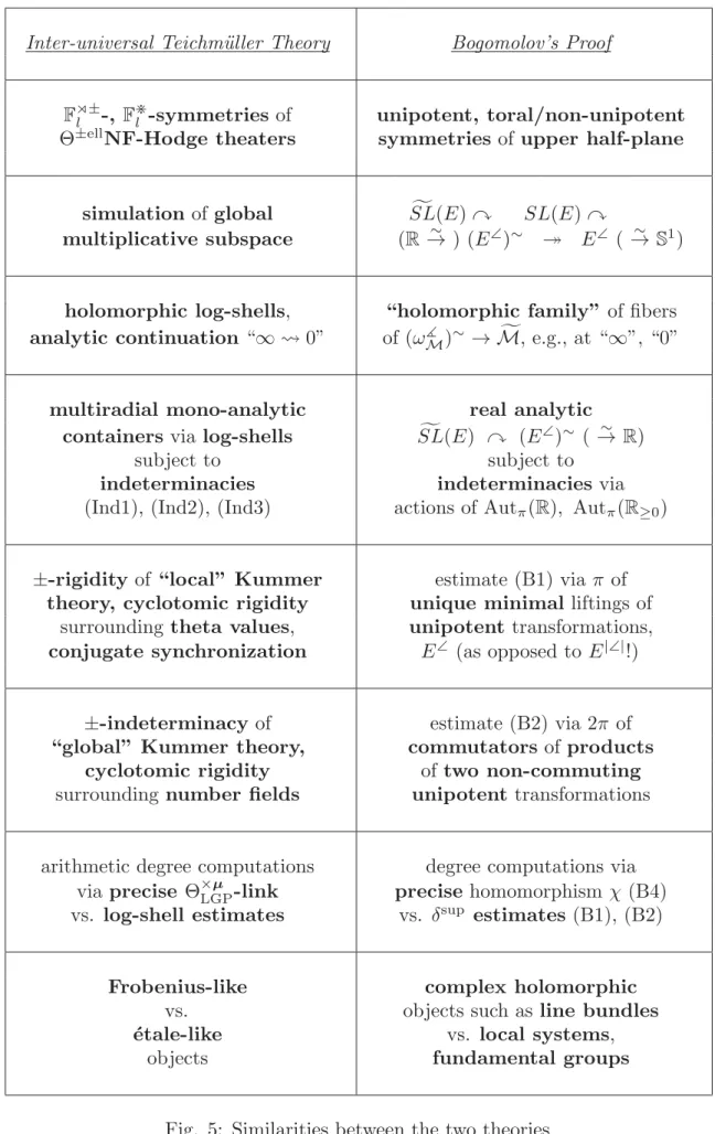
Inter-universal Teichm¨uller Theory Bogomolov’s Proof

F^±_l -, F_l -symmetries of unipotent, toral/non-unipotent Θ^±ellNF-Hodge theaters symmetriesof upper half-plane

simulation of global SL(E) SL(E)

multiplicative subspace (R →^∼ ) (E^∠)^∼ E^∠ ( →^∼ S¹)

holomorphic log-shells, “holomorphic family” of fibers analytic continuation “∞0” of (ω_M )^∼ →M, e.g., at “∞”, “0”

multiradial mono-analytic real analytic containers via log-shells SL(E) (E^∠)^∼ ( →^∼ R)

subject to subject to

indeterminacies indeterminacies via (Ind1), (Ind2), (Ind3) actions of Autπ(R), Autπ(R≥0)

±-rigidity of “local” Kummer estimate (B1) via π of theory, cyclotomic rigidity unique minimal liftings of

surrounding theta values, unipotent transformations, conjugate synchronization E^∠ (as opposed to E^|∠|!)

±-indeterminacy of estimate (B2) via 2π of

“global” Kummer theory, commutatorsof products cyclotomic rigidity of two non-commuting surrounding number fields unipotent transformations

arithmetic degree computations degree computations via via precise Θ^×μ_LGP-link precisehomomorphism χ (B4) vs. log-shell estimates vs. δ^sup estimates (B1), (B2)

Frobenius-like complex holomorphic

vs. objects such as line bundles

´

etale-like vs. local systems,

objects fundamental groups

Fig. 5: Similarities between the two theories

Next, we recall that the suitability of the multiradial mono-analytic containers furnished by log-shells for explicit estimates [cf. [IUTchIII], Remark 3.10.1, (iii)] lies in sharp contrast to the precise, albeit somewhat tautological, nature of the correspondence [cf. (IU2)] concerning arithmetic degrees of objects of interest [i.e., q-pilot and Θ-pilot objects] given by the Θ^×μ_LGP-link [cf. [IUTchIII], Definition 3.8, (i), (ii); [IUTchIII], Remark 3.10.1, (ii)]. This precise correspondence is reminiscent of the precise, but relatively “superficial” [i.e., by comparison to the estimates (B1), (B2)], relationships concerning degrees [cf. (B4)] that arise from the homomorphismχ[i.e., which is denoted “deg” in [Zh]!]. On the other hand, the final estimate (B5) requires one to apply boththe precise computation of (B4) and the nontrivial estimates of (B1), (B2). This state of affairs is highly reminiscent of the discussion surrounding [IUTchIII], Fig. I.8, of two equivalent ways to compute log-volumes, i.e., the precise correspondence furnished by the Θ^×μ_LGP-link and thenontrivial estimatesvia the multiradial mono-analytic containers furnished by the log-shells.

Finally, we observe that the complicated interplay between “Frobenius-like”

and “´etale-like” objects in inter-universal Teichm¨uller theory may be thought of as corresponding to the complicated interplay in Bogomolov’s proof between

complex holomorphic objects such as the holomorphic line bundle ω_M and the natural surjections ω^×_M ω_M^×⊗12 C^× arising from the discriminant modular form

— i.e., which correspond to Frobenius-like objects in inter-universal Teichm¨uller theory — and

the local system EM and the various fundamental groups[and mor- phisms between such fundamental groups such as χ] that appear in Fig.

3

— i.e., which correspond to´etale-like objects in inter-universal Teichm¨uller theory.

The analogies discussed above are summarized in Fig. 5 above.

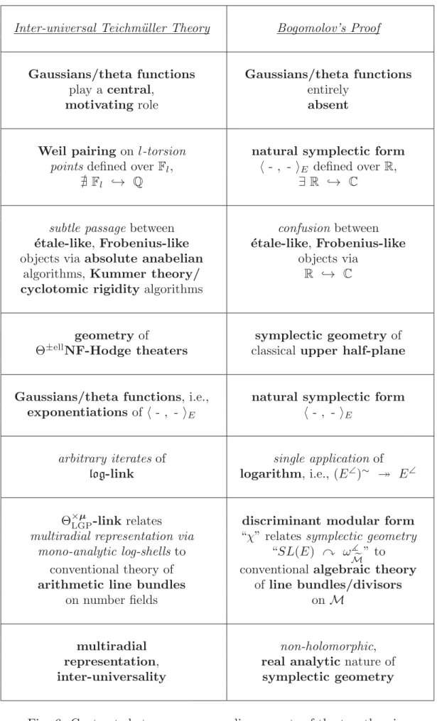
Section 5: Differences Between the Two Theories

In a word, the most essential difference between inter-universal Teichm¨uller theory and Bogomolov’s proof appears to lie in the

absence in Bogomolov’s proof of

Gaussian distributions and theta functions, i.e., which play a central role in inter-universal Teichm¨uller theory.

In some sense, Bogomolov’s proof may be regarded as arising from thegeom- etry surrounding the natural symplectic form

- , - E def

= - , - E|E

on thetwo-dimensional R-vector space E. The natural arithmetic analogue of this symplectic form is theWeil pairingon thetorsion points— i.e., such as the l-torsion points that appear in inter-universal Teichm¨uller theory — of an elliptic curve over a number field.