PAPER
Fast Edge Preserving 2D Smoothing Filter Using Indicator Function
Ryo ABIKO†a),Nonmember andMasaaki IKEHARA†b),Fellow
SUMMARY Edge-preserving smoothing filter smoothes the textures while preserving the information of sharp edges. In image processing, this kind of filter is used as a fundamental process of many applications. In this paper, we propose a new approach for edge-preserving smoothing filter.
Our method uses 2D local filter to smooth images and we apply indicator function to restrict the range of filtered pixels for edge-preserving. To de- fine the indicator function, we recalculate the distance between each pixel by using edge information. The nearby pixels in the new domain are used for smoothing. Since our method constrains the pixels used for filtering, its running time is quite fast. We demonstrate the usefulness of our new edge-preserving smoothing method for some applications.
key words:edge-preserving smoothing, indicator function, denoising, con- tents matching
1. Introduction
Due to the spread of smartphones and SNS, image pro- cessing became more familiar to us and image filtering is used in many applications in image processing and com- puter graphics. In particular, edge-preserving smoothing filter is used in a fundamental process of many kinds of applications in image processing, including clip-art JPEG artifact removal[1],[2], detail manipulation[3]–[5], guided denoising[6],[7], colorization[5],[8],[9], guided upsam- pling[9], [10], tone mapping[3], [4], [11], super resolu- tion[12], depth-of-field effect[5], haze removal[13], and stylization[5].
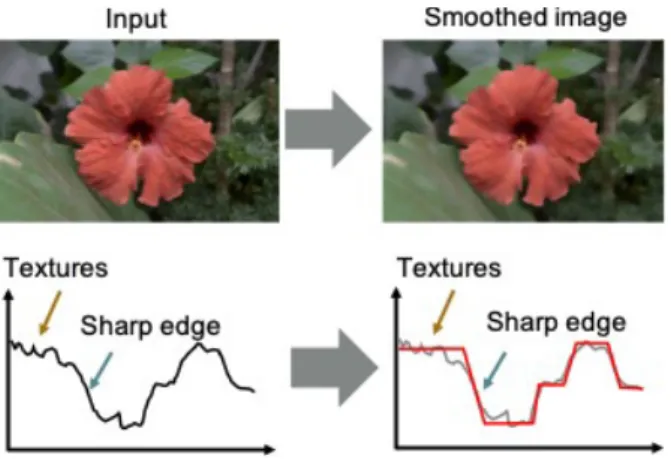
Edge-preserving smoothing filter smoothes the image but when a sharp edge appears, it stops smoothing. It means that the texture region is smoothed but the sharp edge will be preserved. This operation is visualized in Fig. 1. In the field of image processing, to apply a different process to texture region and edge region is important to obtain a high quality image. Since the normal smoothing filter such as Gaussian filter or moving average filter smoothes both texture region and edge region, it is difficult to decompose image into tex- ture region and edge region. On the other hand, since edge- preserving smoothing filter smooths only texture region, it is possible to separate image into texture region and global edge region by taking the difference between the input im- age and smoothed image. It is a reason why edge-preserving
Manuscript received December 21, 2018.
Manuscript revised May 27, 2019.
Manuscript publicized July 22, 2019.
†The authors are with the Department of Electronics and Elec- trical Engineering, Keio University, Yokohama-shi, 223–8522, Japan.
a) E-mail: [email protected] b) E-mail: [email protected]
DOI: 10.1587/transinf.2018EDP7437
Fig. 1 The example of edge-preserving smoothing filter.
smoothing filter is used in many applications.
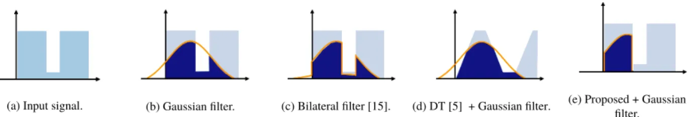
The most popular and classical edge-preserving smoothing filters are anisotropic diffusion[14]and bilateral filter[15]. Anisotropic diffusion applies heat conduction equation on the image and many iterative processes are re- quired. On the other hand, bilateral filter computesL2norm in both spacial and range domain. Therefore, even if there are thin edges in image like in Fig. 3, bilateral filter might refer the pixels over the valley. The cross reference over sharp edges might deteriorate the performance of smooth- ing. To improve the quality of edge-preserving smooth- ing, various methods have been proposed: weighted least squares (WLS)[3], edge-avoiding wavelets (EAW)[16], do- main transform (DT)[5], guided filter (GF)[6], fast global image smoothing (FGS)[9], tree filtering (TF)[17],L0gra- dient minimization (L0GM)[11]andL0gradient projection (L0GP)[2]. The local filtering method can process the image in short time but the edge-preserving effect is not enough.
On the other hand, non-local method likeL0gradient projec- tion[2]can smooth image sufficiently but the running time is quite long.
To overcome the disadvantage of local filter, we pro- pose a new method for performing edge-preserving smooth- ing to images in local filter. Our approach defines the indica- tor function which indicates the pixels used for smoothing.
It is defined in 2D and we use edge information to gather the pixels which belong to the same region. Because the in- dicator function restricts the region of smoothing, our filter will not smooth across the sharp edges. That feature gives us flexibility of which type to use for smoothing such as Simple Moving Average (SMA), Gaussian smoothing filter, etc.
Copyright c2019 The Institute of Electronics, Information and Communication Engineers
indicator function restricts the spatial range of pixels in the filtering, the computational cost is low. Our edge-preserving smoothing filter can smooth the image rapidly due to the constraint of the range and the simplicity of our algorithm.
This result is remarked in Sect. 4. We demonstrate the ap- plications of our edge-preserving smoothing filter in Sect. 5, including clip-art JPEG artifact removal and detail manipu- lation.
2. Supporting Methods
2.1 Bilateral Filter (BF)
A bilateral filter[15] is a most popular edge-preserving smoothing filter. It works by weight averaging the value of neighbor pixels in space and range dimension. If the spa- tial or range distance is long, the weighting factor will be small. In contrast, if the similarity of the pixels is high, the weighting factor will be large. Therefore, the bilateral filter- ing weightwxypqis given by
wxypq= 1 Kxyexp
−p2+q2 σ2s
exp
−(Ixy−Ix+p,y+q)2 σ2r
(1)
Kxy=
p,q∈Ω
exp
−p2+q2 σ2s
exp
−(Ixy−Ix+p,y+q)2 σ2r
(2)
where (x, y) are the coordinates of the target pixel, (p,q) are the offsets in the kernel,Ixyis the pixel value andKxy is a normalization factor which makes the sum of the filter to 1. σsandσrare parameters to decide the sensitivity in the spacial and range dimension. The filtered image valueJxyis computed by
Jxy=
p,q∈Ω
wxypqIx+p,y+q. (3)
Since this method have to compute all weighting factor in the kernel, the computational cost is high. To speed up the process, many approaches have been proposed[18]–[20]but in most cases they need quantization, downsampling or ap- proximation. To overcome these deterioration factor, several methods were also proposed[21],[22].
2.2 Domain Transform (DT)
Domain Transform (DT)[5]is a fast method for the edge- preserving image processing. To speed up the process, it applies 1D domain transform to the image in advance and process the image by 1D filter. The smoothing amount in spatial and range dimension are determined by the parame- terσsandσr, and the 1D transformed domain is given by
Normalized Convolution smoothes image strongly since it simply averages the values of the nearby pixels in the trans- formed domain. The equation of Normalized Convolution is:
Jx=(1/Kx)
p∈D(Ω)
Ix+pH(tx,tx+p)
H(tx,tx+p)=⎧⎪⎪⎨
⎪⎪⎩1 if |tx−tx+p| ≤ √ 3σs
0 otherwise . (5)
Since this method uses 1D-domain transform, it can only apply 1D filter to the images. Therefore, it applies 1D filter to the input image (2D signal) for several times from the dif- ferent direction but it may cause artifacts along the direction which the 1D filter is applied finally. Since the image is pro- cessed as a 1D signal, the output image is not rotationally invariant.
2.3 L0Gradient Projection (L0GP)
L0Gradient Projection (L0GP)[2]minimizes the quadratic data-fidelity term subject to L0 gradient term is less than user-given parameterα.L0gradient term shows the number of non-zero gradient of the output image and the quadratic data-fidelity term shows theL2norm of the input image and the output image. The amount of smoothing is controlled byαwhich determine the weight betweenL0gradient term and quadratic data-fidelity term. To perform the smoothing, a constrained optimization problem has to be solved and the formulation is shown as:
Findu∈argmin
u∈R3N
1
2u−u¯2subject to GradL0(u)≤α.
(6) Since this method minimize theL0 gradient by solving the constrained optimization problem, the image is strongly smoothed but the computational time is quite long.
3. Proposed Method
We define a new 2D filter composed of smoothing term and indicator term. Since the indicator function constrains the range of smoothing, it improves the edge-preserving effect and speeds up the running time. The example of our filter weights are shown in Fig. 2. Before computing the indicator term, we compute the reconstructed distance of pixels by integrating the edge information. The indicator function is defined by judging if the reconstructed distance of the pixels is smaller than the user-given parameterσ.
Fig. 3 Visualization of the filter weights and the convolution when a sharp edge exists in the image.
Fig. 2 The example of our filtering weights.
3.1 Indicator Function
When the edge-preserving smoothing is performed, it is im- portant to smooth the pixels which belong to the same re- gion. However, classic smoothing filter (e.g. moving aver- age, Gaussian smoothing filter or bilateral filter[15]) might smooth across different regions because they only refer to the space or intensity information. This characteristic dete- riorates the performance of smoothing. Therefore, we define Hxypqas an indicator function. It indicates the pixels which are in the same region. From the above, our filtering weight wxypqand indicator termHxypqare expressed as:
wxypq= 1
KxySxypqHxypq (7) Hxypq=⎧⎪⎪⎨
⎪⎪⎩1 if rxypq≤σ
0 otherwise , (8)
whereSxypq is a smoothing term andrxypq is a distance of two pixels in the reconstructed domain, which is explained in Sect. 3.2. Kxy is a normalization factor which makes the sum of the filter to 1. σis a user-given parameter which determines the size of region and it also determines the amount of smoothing. When we use Simple Moving Aver- age (SMA) for the smoothing term, the maximum smooth- ing effect is obtained. In that case, our filtering weight can be expressed as
wSMAxypq = 1 KxySMA
Hxypq. (9)
Since the computational cost is low, we mainly use (9) for the experiments. Our final smoothed image JEPFIFxyc is ob- tained by applying filter to RGB color space as following equation.
Fig. 4 The visualized image of computing reconstructed domain.
JEPFIFxyc =
p,q∈Ω
wxypqIx+p,y+q,c. (10)
3.2 Reconstructed Domain
Our indicator function judges whether pixels are in the same region or not by the information of edges. When a sharp edge exists between two pixels, the pixels should be classi- fied into different regions. Thus, we recalculate the distance of each pixels by integrating the intensity of edge informa- tion. We call this new domain as Reconstructed domain. In reconstructed domain, the distance of two pixels should be larger if more edges exist between them. The similar ap- proach was proposed in DT[5] but this method was only available in 1D signal. Since there are no solution for 2D signals to define the accurate domain transform[5], we de- fine the reconstructed domain by integrating the information of edges in a limited situation.
Considering the case of 2D signal, there are many routes for integrating edge information and each of them may have different values. In order to reduce the compu- tational cost, only two routes are computed in our method.
The example of two routesLxypq1 andLxypq2are shown in Fig. 4 (a). When (p,q) are both positive, Lxypq1 andLxypq2
are given by following expressions:
Npq ={N0,N1,· · · ,Np,Np+1,· · ·,Nk}
={Ix,y,Ix+1,y,· · · ,Ix+p,y,Ix+p,y+1,· · · ,Ix+p,y+q} Lxypq1=
c
k l=1
|Nl−Nl−1|
Mpq ={M0,M1,· · ·,Mq,Mq+1,· · ·,Mk}
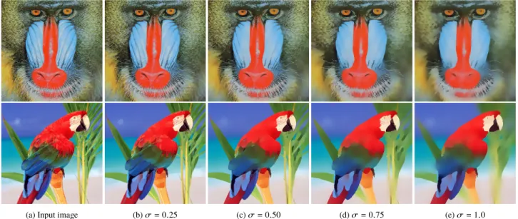
Fig. 5 The comparison of the results when variousσis selected. Equation (9) is used for the process and the filter size is 9×9. Three iterations are performed.
={Ix,y,Ix,y+1,· · · ,Ix,y+q,Ix+1,y+q,· · ·,Ix+p,y+q}
Lxypq2=
c
k l=1
|Ml−Ml−1|. (11)
N and M are the sorted pixels on the each route andk =
|p|+|q|is the number of pixels in each route. When (p,q) are not positive, the sign of (11) must be appropriately in- verted. The information on color channel is integrated when we calculateLxypq1andLxypq2. This process is visualized in Fig. 4 (b). DT use the information of space domain in or- der to define the accurate domain transform but in (11), the space information is not integrated since it is not important for our method.
To calculate (11) in every kernel will cost high com- putational resource. Thus, our method calculates 1D edge integrated values in advance. The integration in (11) can be calculated easily by using this value. The 1D edge integrated valuesLXxyandLYxyare expressed as:
LXxy=
c
x i=1
|Iiy−Ii−1,y|
LYxy=
c
y i=1
|Ixi−Ix,i−1|.
(12)
Applying (12) to (11), the two routes are given by:
Lxypq1=|LXx+p,y−LXxy|+|LYx+p,y+q−LYx+p,y|
Lxypq2=|LYx,y+q−LYxy|+|LXx+p,y+q−LXx,y+q|. (13) Because classifying as many pixels as possible in the same region is important for smoothing, we define the smaller value of Lxypq1 and Lxypq2 as the distance of two pixels in the reconstructed domain. Therefore, the distance rxypqof the two pixels in the reconstructed domain is defined
by (14).
rxypq=min(Lxypq1,Lxypq2) (14) We revealed experimentally that using two routes for calcu- lating distance in reconstructed domain shows a good trade- offbetween edge-preserving quality and the computational cost.
Figure 3 shows the 1D signal and the weighting factor of some smoothing methods. The methods which can be classified as a local filter are shown in the figure. We can see that conventional methods smooth over the sharp edge but our method does not refer to the information over the edge.
It is because our method constrains the region of smoothing by the indicator term and it leads to efficient edge-preserving smoothing.
3.3 Parameters Analysis
Since we define the smoothing term and the indicator func- tion separately, our filter can smooth images flexibly. When σ is large enough, the indicator function always take the value of 1. Thus, our filter acts like conventional smoothing methods: simple moving average filter (SMA), Gaussian fil- ter, and the bilateral filter. In contrast, whenσis set to an ap- propriate value, the filter acts as an edge-preserving smooth- ing filter. In this case, the method chosen for the smoothing term determines the amount of smoothing. We mainly use (9) as our filter since it can obtain the best smoothing ef- fect. The difference occurred by the choice ofσis shown in Fig. 5. Whenσis set to a small value, the smoothing effect is limited and some texture remains. In contrast, when σ is set to a large value, our filter smoothes over edges. The suitable parameter ofσis depended on the applications.
Since indicator function takes the sum of the pixel dif- ferences, the further pixels tend to be classified to a different
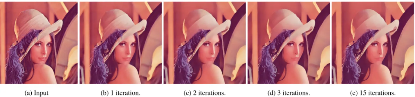
Fig. 7 The comparison between the number of iterations. Equation (9) is used for the process,σ= 0.45 and the filter size is 9×9. The result of 3 iterations is quite similar to 15 iterations, during the results of 1 and 2 iterations do not have enough smoothing effect.
Fig. 6 The PSNR between the original image and the smoothed image in each iteration.σ=0.50, the filter size is 9×9.
region. In order to overcome this problem, we apply our fil- ter to the image for several times. When the number of iter- ation increases, more smoothed image is outputted but when we use the same value ofσduring the iterations, too much smoothing effect is obtained. Experimentally we decide to reduce the value ofσby half through iterations.
σit=(0.5(t−1))σ (15)
where σit is the parameter used in t-th iteration. The re- sult image oft-th iteration is used for the input of (t+1)- th iteration. In most cases, when the number of iterations gets larger than 3, the change of the PSNR[23]between the non-smoothed image and the smoothed image will be small enough (Fig. 6). Therefore, we decide to perform 3 iterations for our method. The visual results with different numbers of iterations are shown in Fig. 7.
4. Experimental Results
In this section, we show the smoothed image processed by our method and the comparison methods. The comparison methods are Domain Transform (DT)[5],L0Gradient Pro- jection (L0GP)[2] and bilateral filter (BF)[15]. The edge- preserving smoothing result to 5 images are shown in Fig. 8.
Analyzing the results of DT andL0GP in Fig. 8, some artifacts are observed in vertical and horizontal direction when preserving diagonal edges. In contrast, the artifact
does not appear in our method. It is because our method applies 2D indicator function and it has flexibility in pre- serving complex edges. In addition, we can see that DT and BF cannot preserve thin edges but our method can preserve them. The usefulness of our indicator function is shown by comparing the results in Fig. 8 (d) and Fig. 8 (f). Figure 8 (d) is the output of bilateral filter and Fig. 8 (f) is the output of proposed method which uses bilateral filter as the smooth- ing kernel. Bilateral filter smoothes over edges as shown in Fig. 8 (d) but Fig. 8 (f) shows the effective smoothing re- sult which does not smoothes over edges and preserves thin edges.
Our method can process 1M pixel RGB image in 0.25 seconds on quad core [email protected] with our C++imple- mentation. Equation (9) is used in the computation, filter size is set to 9 and the number of iterations are 3. When we do not use Eq. (12) and Eq. (13) for the speeding up, the running time will be 3.2 times slower. Since our method is classified to local filter, parallel coding is effective for de- creasing the execution time. The comparison of the execu- tion time is shown in Table 1.
5. Applications
Since edge-preserving smoothing filter smooths only texture region, it is mainly used to separate the texture from the im- age. This feature is used in many applications. For exam- ple, detail manipulation is performed by adding enhanced texture information to the smoothed image. Guided denois- ing, colorization, guided upsampling, tone mapping, depth- of-field effect, haze removal, stylization and clip-art JPEG artifact removal are also available as applications.
The example of clip-art JPEG artifact removal is shown in Fig. 9. Since edge-preserving smoothing filter preserves sharp edges, it can be used for the preprocess method of image segmentation.
The comparison of segmentation result between pre- processed image and normal image is shown in Fig. 10.
SLIC[26]is used for the segmentation. We can see that the segmented result after smoothed by our method can track the edge more effectively. The result of edge/boundary de- tection evaluation on 100 test images in BSDS300 is shown in Fig. 11. We can see that the F-measure got better when
Fig. 8 Image smoothing results comparison with DT[5](σs=40,σr=0.4),L0GP[2](α=0.25N) and BF[15](σs =20,σr =0.07). Figure 8 (e) and Fig. 8 (f) are the result of proposed method. σis set to 0.35 in both Fig. 8 (e) and Fig. 8 (f). We use SMA as the smoothing term (defined in Eq. (9)) in Fig. 8 (e) while BF (σr=0.07σs=20) in Fig. 8 (f). The filter size of Proposed method are set to 9×9.
3 iterations are performed in all methods exceptingL0GP. The same parameters are used to process each image.
Table 1 The comparison of the computational time for 512×512 RGB image. The comparison methods are Bilateral Filter (σs = 20, σr = 0.07)[15],L0Gradient Minimization (λ=0.0015)[11],L0Gradient Pro- jection (α=0.08N,γ=3,η=0.95)[2], Domain Transform (σs =40, σr=0.4)[5], Fast Global Image Smoothing (λ=50,σ=0.1)[9]and our proposed method (filter size: 9×9,σ=0.5).
BF L0GM L0GP DT FGS Ours
MATLAB 1.52 s 1.46 s 102 s 2.89 s - 1.70 s
C++ - - - 0.04 s 0.15 s 0.07 s
we applied our method before applying SLIC to the images.
Since we define the indicator function in 2D space, our method is rotationally invariant. TheL0error rate are shown in Table 2. TheL0 error rate of image J1 and J2 can be expressed as:
Fig. 9 The result of denoising applied on JPEG image.
E= 1 N
x,y
δ(Jx1y−J2xy)
Fig. 10 The comparison of image segmentation result.
Fig. 11 The result of edge/boundary detection evaluation. The parameter is set toσ=0.45 and the filter size is 9×9. The higher is the better.
Table 2 The comparison ofL0error rate between the output images pro- cessed by 90 degrees rotated input and normal input. The result is ex- pressed in percent. The comparison methods areL0Gradient Minimization (λ=0.0015)[11],L0Gradient Projection (α=0.08N,γ=3,η=0.95)[2], Domain Transform (σs=40,σr=0.4)[5], Fast Global Image Smoothing (λ=50,σ=0.1)[9]and our proposed method (filter size: 9×9,σ=0.5).
Dataset name L0GM L0GP DT FGS Ours BSDS300[24] 0.29 0.92 0.25 0.25 0.00 COCO[25] 0.31 0.42 0.27 0.26 0.00
Average 0.30 0.67 0.26 0.26 0.00
δ(a)=⎧⎪⎪⎨
⎪⎪⎩1 a0
0 a=0. (16)
where N is the pixel number and x,yare the coordinates.
When two images are completely same, the error rate will be 0. The result in Table 2 shows that our method is rotationally invariant. This feature is available in contents matching in a database system.
6. Conclusion
In this paper, we propose a new approach for the edge- preserving smoothing. We define the 2D indicator function to restrict the pixels which are used for smoothing. This function is defined by comparing the value of the integra- tion of edge information and it is easily computed by us-
ing 1D integration. Because the 1D edge integration can be computed beforehand, the computational cost is low and also parallel implementation is available. Due to defining the indicator function in 2D space, the output of our filter is rotationally invariant. This feature is desirable in case of using our filter in content matching.
References
[1] L. Zhao, H. Bai, A. Wang, and Y. Zhao, “Iterative range-do- main weighted filter for structural preserving image smoothing and de-noising,” Multimedia Tools and Applications, vol.78, no.1, pp.47–74, 2019.
[2] S. Ono, “L0 gradient projection,” IEEE Trans. Image Process., vol.26, no.4, pp.1554–1564, April 2017.
[3] Z. Farbman, R. Fattal, D. Lischinski, and R. Szeliski, “Edge-preserv- ing decompositions for multi-scale tone and detail manipulation,”
ACM SIGGRAPH 2008 Papers, SIGGRAPH ’08, New York, NY, USA, pp.67:1–67:10, ACM, 2008.
[4] K. Subr, C. Soler, and F. Durand, “Edge-preserving multiscale im- age decomposition based on local extrema,” ACM SIGGRAPH Asia 2009 Papers, SIGGRAPH Asia ’09, New York, NY, USA, pp.147:1–147:9, ACM, 2009.
[5] E.S.L. Gastal and M.M. Oliveira, “Domain transform for edge-aware image and video processing,” ACM Transactions on Graphics (ToG), vol.30, no.4, ACM, 2011.
[6] K. He, J. Sun, and X. Tang, “Guided image filtering,” IEEE Trans.
Pattern Anal. Mach. Intell., vol.35, no.6, pp.1397–1409, June 2013.
[7] G. Deng, “Guided wavelet shrinkage for edge-aware smoothing,”
IEEE Trans. Image Process., vol.26, no.2, pp.900–914, Feb. 2017.
[8] A. Levin, D. Lischinski, and Y. Weiss, “Colorization using op- timization,” ACM Transactions on Graphics (ToG), vol.23, no.3, pp.689–694, ACM, 2004.
[9] D. Min, S. Choi, J. Lu, B. Ham, K. Sohn, and M.N. Do, “Fast global image smoothing based on weighted least squares,” IEEE Trans. Im- age Process., vol.23, no.12, pp.5638–5653, Dec. 2014.
[10] K.-H. Lo, Y.-C.F. Wang, and K.-L. Hua, “Edge-preserving depth map upsampling by joint trilateral filter,” IEEE Trans. Cybern., vol.48, no.1, pp.371–384, Jan. 2018.
[11] L. Xu, C. Lu, Y. Xu, and J. Jia, “Image smoothing viaL0gradient minimization,” Proceedings of the 2011 SIGGRAPH Asia Confer- ence, SA ’11, New York, NY, USA, pp.174:1–174:12, ACM, 2011.
[12] S. Huang, J. Sun, Y. Yang, Y. Fang, P. Lin, and Y. Que, “Ro- bust single-image super-resolution based on adaptive edge-preserv- ing smoothing regularization,” IEEE Trans. Image Process., vol.27, no.6, pp.2650–2663, June 2018.
[13] D. Park, D.K. Han, and H. Ko, “Single image haze removal with wls-based edge-preserving smoothing filter,” 2013 IEEE Interna- tional Conference on Acoustics, Speech and Signal Processing, pp.2469–2473, May 2013.
[14] P. Perona and J. Malik, “Scale-space and edge detection using anisotropic diffusion,” IEEE Trans. Pattern Anal. Mach. Intell., vol.12, no.7, pp.629–639, 1990.
[15] C. Tomasi and R. Manduchi, “Bilateral filtering for gray and color images,” Sixth International Conference on Computer Vision (IEEE Cat. no.98CH36271), pp.839–846, Jan. 1998.
[16] R. Fattal, “Edge-avoiding wavelets and their applications,” ACM Trans. Graph., vol.28, no.3, pp.1–10, 2009.
[17] L. Bao, Y. Song, Q. Yang, H. Yuan, and G. Wang, “Tree filtering:
Efficient structure-preserving smoothing with a minimum spanning tree,” IEEE Trans. Image Process., vol.23, no.2, pp.555–569, 2014.
[18] S. Paris and F. Durand, “A fast approximation of the bilateral filter using a signal processing approach,” International Journal of Com- puter Vision, vol.81, no.1, pp.24–52, Jan. 2009.
[19] K.N. Chaudhury, D. Sage, and M. Unser, “FastO(1) bilateral filter- ing using trigonometric range kernels,” IEEE Trans. Image Process.,
tion of edge-preserving filtering on cpu microarchitectures,” Applied Sciences, vol.8, no.10, 2018.
[23] A. Hore and D. Ziou, “Image quality metrics: PSNR vs.
SSIM,” 2010 20th International Conference on Pattern Recognition, pp.2366–2369, Aug. 2010.
[24] D. Martin, C. Fowlkes, D. Tal, and J. Malik, “A database of human segmented natural images and its application to evaluating segmen- tation algorithms and measuring ecological statistics,” Proc. 8th Int’l Conf. Computer Vision, pp.416–423, July 2001.
[25] T.-Y. Lin, M. Maire, S. Belongie, J. Hays, P. Perona, D. Ramanan, P. Doll´ar, and C.L. Zitnick, “Microsoft coco: Common objects in context,” Computer Vision – ECCV 2014, ed. D. Fleet, T. Pajdla, B. Schiele, and T. Tuytelaars, Cham, pp.740–755, Springer Interna- tional Publishing, 2014.
[26] R. Achanta, A. Shaji, K. Smith, A. Lucchi, P. Fua, and S.
S¨usstrunk, “Slic superpixels compared to state-of-the-art superpixel methods,” IEEE Trans. Pattern Anal. Mach. Intell., vol.34, no.11, pp.2274–2282, 2012.
Ryo Abiko received the B.E. degrees in elec- trical engineering from Keio University, Yoko- hama, Japan, in 2018. He is currently an M.E.
student at Keio University, Yokohama, Japan, under the supervision of Prof. Masaaki Ikehara.
His research interests are in the field of image filtering, denoising and image processing using deep learning.
Masaaki Ikehara received the B.E., M.E.
and Dr.Eng. degrees in electrical engineering from Keio University, Yokohama, Japan, in 1984, 1986, and 1989, respectively. He was Ap- pointed Lecturer at Nagasaki University, Naga- saki, Japan, from 1989 to 1992. In 1992, he joined the Faculty of Engineering, Keio Univer- sity. From 1996 to 1998, he was a visiting re- searcher at the University of Wisconsin, Madi- son, and Boston University, Boston, MA. He is currently a Full Professor with the Department of Electronics and Electrical Engineering, Keio University. His research interests are in the areas of multi-rate signal processing, wavelet image coding, and filter design problems.
![Fig. 8 Image smoothing results comparison with DT [5] ( σ s = 40, σ r = 0 . 4), L 0 GP [2] ( α = 0](https://thumb-ap.123doks.com/thumbv2/123deta/5629952.1500910/6.892.81.818.113.747/fig-image-smoothing-results-comparison-dt-σ-gp.webp)

