Performance Analysis of the Interval Algorithm for Random Number Generation in the Case of Markov Coin Tossing ∗

(1)

PAPER

Special Section on Information Theory and Its Applications

Performance Analysis of the Interval Algorithm for Random Number Generation in the Case of Markov Coin Tossing ^∗

Yasutada OOHAMA^†a),Senior Member

SUMMARY In this paper we analyze the interval algorithm for random number generation proposed by Han and Hoshi in the case of Markov coin tossing. Using the expression of real numbers on the interval [0,1), we first establish an explicit representation of the interval algorithm with the representation of real numbers on the interval [0,1) based one number systems.

Next, using the expression of the interval algorithm, we give a rigorous analysis of the interval algorithm. We discuss the difference between the expected number of the coin tosses in the interval algorithm and their upper bound derived by Han and Hoshi and show that it can be characterized explicitly with the established expression of the interval algorithm.

key words: random number generation, interval algorithm, Markov coin tossing, number systems, performance analysis

1. Introduction

Simulation problems of generating random sequences from a prescribed information source by using a random sequence from a given information source are called the random number generation. In the random number generation random sequences from a prescribed information sources are called thetargetrandom sequences which we wish toproduceand the random sequence from given information sources are called thecoinrandom sequences that the target random sequences aremade from.

There have been several works on the random number generation in the field of computer science and information theory. Some interesting relations between random number generation and information theory have been found in the papers of Elias[1]and Knuth and Yao[2].

Han and Hoshi[3]studied a variable-to-fixed random number generation problem. They studied the method of generating target random sequences of fixed length from a prescribed information source by using coin random sequences ofvariable lengthfrom a given information source.

They proposed a simple algorithm called the interval algorithm and obtained results for its performance analysis.

When coin random sequences are from a stationary memoryless source, Han and Hoshi[3] established an upper bound of the average length of coin random sequences necessary to create target random sequences. The derived

Manuscript received January 25, 2020.

Manuscript revised June 1, 2020.

†The author is with The University of Electro-Communications, Chofu-shi, 182-8585 Japan.

∗This work was presented in part at the Symposium on Nonlin- ear Theory and Its Applications (NOLTA2016), Yugawara, Japan, Nov. 27–30, 2016.

a) E-mail: [email protected]

DOI: 10.1587/transfun.2020TAP0008

bound is characterized with a fraction of two entropies of given and prescribed sources and is shown to be asymptot- ically optimal for large length of output sequences. They further studied an extended case, where coin random sequences are from a stationary Markov information source.

We hereafter call the stationary Markov information sources which outputs coin random sequences the Markov coin tossing. Han and Hoshi[3]also investigated a random number generation problem of generating a prescribed target random process using a given coin random process. Watanabe and Han[4]investigated this random generation problem by the information spectrum approach[5].

In [6], the author studied the performance analysis of the interval algorithm for random number generation proposed by Han and Hoshi[3]. Using representation of real numbers, the author refined Han and Hoshi’s performance analysis of the interval algorithm. In the above work the author treated the problem that we wish to generate a target random variable by using a coin random sequence from a stationary memoryless source.

In this paper we analyze the interval algorithm for random number generation proposed by Han and Hoshi[3]in the case of Markov coin tossing. We extend the method developded by the author[6] to this case, deriving several explicit results.

As a theoretical extension we have an importance on the study of the random number generation problem in the case of Markov coin tossing. We also have a practical importance on this study. From a practical point of view information resources which output coin random sequence must be easily accessible and available. On the other hand, information resources in the real world that we can easily ac- cess to utilize include several data such as text data, digi- tally processed audio, image or video data. Most of them have memory and are mathematically modeled by Markov information sources. Hence, considering applications of the random number generation in practical situations such that we only have a few choices of information resources available as generators of coin random sequences, we inevitably face to the study of the random number generation in the case of Markov coin tossing.

In this paper we derive explicit results on the performance analysis of the interval algorithm for random number generation using an expression of real numbers in the unit interval [0,1). On the expression of real numbers in the unit interval, we establish a kind of generalized number system based on the stochastic structure of the coin random pro- Copyright c2020 The Institute of Electronics, Information and Communication Engineers

(2)

1326

cess. Using the above representation of real numbers on the interval, we find an explicit expression of the interval algorithm. We further present a rigorous analysis of the interval algorithm using the expression of the algorithm.

We discuss the difference between the expected number of the coin tosses in the interval algorithm and their upper bound derived by Han and Hoshi and show that it can be characterized explicitly with the established expression of the interval algorithm.

An explicit representation of the interval algorithm de- veloped by the author [6] can be extended to the case of Markov coin tossing. However, this case yields some specific difficulty in the performance analysis of the interval algorithm. To state this difficulty we define a mapϕrepre- senting the interval algorithm. We further define a random variableS which generates the target random variableXby ϕ, that is,ϕ(S)=X. Precise definitions of those quantities will be stated in Sects. 2 and 4. Performance of the interval algorithm is measured by an expected number of coin tossing denoted by ¯L. In the case where coin random sequences are from a stationary memoryless source we have H(S) = LH, where¯ H is the entropy rate of the descrete memoryless source. In this case the performance analysis for the interval algorithm is reduced to an evaluation of H(S). However, as stated in[3], this equality does not hold in general in the case of Markov coin tossing. In this paper we present a class of stationary Markov information sources having asymmetrical propertyon their stochastic matrices.

We prove that for Markov information sources belonging to this class the above equality holds. For Markov information sources not belonging to this class, another method of evaluating ¯Lwill be necessary.

The results of this paper were presented in part at[7], where several arguments are omitted because of page con- straint. Furthermore, it contains a mistake. In this paper we provide those arguments and give a complete proof of our main result on the performance analysis of interval algorithm. We also fix the above mistake in[7].

2. Interval Algorithm for Random Number Genera- tion

LetXbe random variables taking values in a finite setX:= {0,1,· · ·,N −1}. Let p_X := {p_X(x)}x∈X be a probability distribution ofX. Let{Yt}^∞_t₌₁be a stationary Markov source.

For eacht = 1,2,· · ·,Y_t takes values in a finite setY := {0,1,· · · ,M−1}. The stationary Markov source{Yt}^∞_t₌₁is specified with theM×Mstochastic matrix denoted byP= [Pi j], where

Pi j=Pr{Yt+1= j|Yt=i},fort=1,2,· · ·.

We also writePi j,(i,j)× Y²asPi j=pY(j|i). LetY^∗denote the set of all finite sequence emitted from the above information source. We write a string from information source asy^m_l :=y_ly_l₊₁· · ·y_m ∈ Y^∗. Ifl >m, the stringy^m_l means nullstring denoted byλ. Whenl =1, we frequently omit the suffix 1 ofy^m₁ and writey^m = y₁y₂· · ·y_m. Let pY(y^m_l)

denote the probability ofy^m_l . Since the information source is a stationary Markov source, we have

pY(y^m_l )=pY(yl)Py_ly_l+1· · ·Py_m−1y_m.

Here{pY(a)}_a∈Yis a stationary distribution computed from P. The probability of the null stringλassumes to be one.

In this paper we deal with the variable to fixed random number generation problem of generating target random variable X by using the coin random sequence Y1

Y₂· · ·Y_i· · · from a stationary Markov information sources {Yt}^∞_t₌₁. A formal definition of the variable to fixed random number generation problem is the following. Repeated tosses of the coin random variable Y produces random se- quenceY1,Y2,· · · from a Markov source. The coin toss ter- minates at some finite timeLto generate a random variable X with a prescribed distribution pX. L is a random variable specified in terms of a deterministic two valued function such that f(Yⁱ) =‘Continue’ for 1 ≤ i ≤ L−1 and f(Y^L) =‘Stop’. The output X is expressed as X = ψ(Y^L) with some deterministic functionψ.

For the given generating algorithm (f, ψ) of random number generation letS_x,x∈ Xbe a set of all input strings y^l ∈ Y^∗ that generate x. It is obvious thatS_x,x ∈ X are disjoint. Set

S:=X

x∈X

S_x,

where we have used the notation ‘P’ for the sum of disjoint sets instead of ‘∪’. Hereafter, to distinguish the sum of disjoint sets from the union of sets, we use the notation ‘+’ or

‘P’ for the sum ofdisjointsets.

In the above random number generation problem Han and Hoshi [3] proposed a simple algorithm called interval algorithm and evaluated its performance. Let I = [0,1).

Define the cumulative probabilities forpYby cY(0) :=0,

cY(y) :=X

i<y

pY(i),1≤y≤M−1.

Using these probabilities, define the decomposition ofIby IY(y) :=[cY(y),cY(y)+pY(y)).

For pX, we use the same notations and definitions as those forpY. For giveny1∈ Y, define the cumulative probabilities for pY(·|y1)={pY(y2|y1)}_y₂_∈Yby

cY(0|y1) :=0, cY(y2|y1) :=X

i<y2

pY(i|y1),1≤y2 ≤M−1.

Fork=1,2,· · ·, and any stringy^k =y1y2· · ·yk ∈ Y^k, define the semi-open intervalIY(y^k) :=[LY(y^k),UY(y^k)) by the following recursions:

L_Y(y1)=c_Y(y1),

UY(y1)=cY(y1)+pY(y1)

LY(yⁱ)=LY(yⁱ⁻¹)+pY(yⁱ⁻¹)cY(yi|yi−1), UY(yⁱ)=LY(yⁱ)+pY(yⁱ), for 2≤i≤k.











(1)

(3)

The procedure of computing upper and lower end points of the interval corresponding to a given sequence is equivalent to the encoding algorithm in the arithmetic coding. On intervals generated by the above recursion we have the following property.

Property 1: For anyn ≥2, anyaⁿ ∈ Yⁿ, we have that for any 1≤m≤n−1,

[LY(a^m),LY(aⁿ))=

n

X

k=m+1

X

y<a_k

IY(a^k−1y), (2)

[U_Y(aⁿ),U_Y(a^m))=

n

X

k=m+1

X

y>a_k

I_Y(a^k−1y). (3) Proof of Property 1 is given in Appendix. This property will be a basis of a key important result, which yields an explicit representation of the interval algorithm. We derive this key result in the next section.

Interval algorithm by Han and Hoshi[3]can be stated in the following.

Interval Algorithm (Han and Hoshi[3]):

1) Seti=k=1,y0=λ.

2) Givenyi−1, generate a letteryi ∈ Yaccording to the transition probability p_Y(y_i|yi−1) of the coin random variable. Here for i = 1, the quantity pY(y1|y0) = p_Y(y₁|λ) = p_Y(y₁) is the stationary probability of the coin random variable.

3) ComputeI_Y(yⁱ)=[L_Y(yⁱ),U_Y(yⁱ)) according to the recursion (1).

4) IfIY(yⁱ)⊆IX(x) for somex∈ X, then outputxas the value of target random variableX and stop the algorithm.

5) Seti=k+1 and go to 2).

In the above interval algorithm the target random vari- ableXcan exactly be produced.

3. An Explicit Representation of the Interval Algo- rithm

In this section we give two expressions of real numbers in the intervalI=[0,1) on the number system. There is some complementary relation between the above two expressions.

Using those expressions we give an explicit form of the interval algorithm.

3.1 Representation of Real Numbers Forz∈[0,1), define the sequence{ai}^∞_i

=1∈ Y^∗such that z∈IY(aⁱ),i=1,2,· · ·.

It can easily be verified that usinga1,a2,· · ·,zcan be expressed in the following manner:

z=X

k≥1

p_Y(a^k−1)X

a<ak

p_Y(a|ak−1)

=X

k≥1

pY(a^k−1)cY(ak|ak−1).

Here we assume thata0 = λfork = 1. The same rule of notation will be used in the subsequent arguments. We call the above expression the p_Y-ary representation of the real number zand write as

z=0.a₁a2a3· · ·. (4)

In the above expression, if we wish to expresszwith the sum of the number having the expression

0.a₁a2a3· · ·at00· · ·

and the other remaining term, we write

z=0.a1a2· · ·at + 0.0a₁0a₂· · ·0a_tat+1· · · , (5) where the second term is defined by

0.0_a₁0_a₂· · ·0_a_ta_t₊₁· · ·:=X

k≥t+1

p_Y(a^k−1)c_Y(a_k|a_k−1).

Next, forz∈[0,1), set ¯z=1−z. Using the sequence{ai}_i≥1 appearing in thepY-ary representation of the real numberz,

¯

zhas an expression

¯ z=X

k≥1

pY(a^k−1)X

a>ak

pY(a|ak−1).

Then, adopting the notation cY(¯a|ak−1) :=X

i>a

pY(i|ak−1), we obtain the following expression

¯ z=X

k≥1

p_Y(a^k−1)c_Y(¯a_k|ak−1).

We call the above expressionthe pY-ary co- representation of the real number z and write as

¯

z=0.¯a₁a¯₂a¯₃· · ·. (6)

Letz⁽ⁿ⁾denote the real number which is obtained by rounding offzton-digits in thepY-ary representation, that is,

z⁽ⁿ⁾:=0.a1a2· · ·an.

Similarly, let ¯z⁽ⁿ⁾ denote the real number which is obtained by rounding offz¯ton-digits in thepY-ary co-representation, that is,

¯

z⁽ⁿ⁾:=0.¯a₁a¯₂· · ·a¯_n.

It can easily be verified that the pY-ary representation and the pY-ary co-representation of the real number zsatisfy the following.

Property 2:

a) For anyi,z∈IY(aⁱ).

b) cY(a_i|ai−1)+cY(¯ai|ai−1)=1−pY(a_i|ai−1).

(4)

1328

c) Forz=0.a1a2· · ·a_n· · · ∈[0,1),we have z⁽ⁿ⁾+z¯⁽ⁿ⁾=1−p_Y(aⁿ).

From Properties 1 and 2, we have the following lemma.

Lemma 1: We assume thatzhas the followingpY-ary expression:

z=0.a₁a2· · ·an· · · ∈[0,1).

Then for anym≥1, we have the following:

[L_Y(a^m),z)= X

k≥m+1

X

y<ak

I_Y(a^k−1y), (7) [z,UY(a^m))= X

k≥m+1

X

y>a_k

IY(a^k−1y). (8) Proof:By Property 1, we have

[L_Y(a^m),z⁽ⁿ⁾)=[L_Y(a^m),L_Y(aⁿ))

=

n

X

k=m+1

X

y<ak

IY(a^k−1y), (9)

[z⁽ⁿ⁾+p_Y(aⁿ),U_Y(a^m))=[U_Y(aⁿ),U_Y(a^m))

=

n

X

k=m+1

X

y>ak

IY(a^k−1y). (10)

Note that

n→∞limz⁽ⁿ⁾= lim

n→∞(z⁽ⁿ⁾+pY(aⁿ))=z.

Hence by lettingn→ ∞in (9) and (10), we have [LY(a^m),z)= X

k≥m+1

X

y<ak

IY(a^k−1y), [z,U_Y(a^m))= X

k≥m+1

X

y>a_k

I_Y(a^k−1y),

completing the proof.

Lemma 1 plays an important role in deriving an explicit representation of the interval algorithm. The detail of derivation is stated in Sect. 5.

Kanaya[8], Oohama et al.[9] point out that the pY- ary representation has a close connection with the arithmetic coding and the Markov shift. In the following we explain this connection. LetAbe a set ofy²∈ Y²such thatpY(y²)>

0.Note that X

y²∈A

IY(y²)=I,X

y∈Y

IY(y)=I.

Defineτ_Y:I→Iandφ_Y:I→ Yby τY(z)=(pY(y1|y2))⁻¹

z−LY(y²)

+LY(y1), fory²∈ Aandz∈IY(y²),

φY(z)=y, fory∈ Yandz∈IY(y).

The mapτ_Y is called the Markov shift in the terminology

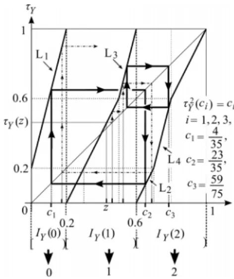
Fig. 1 The mapsτY andφYforPgiven by (11). The quantitiesc1 = 4/35,c₂=23/35, andc₃=59/75 satisfiesτ²_Y(ci)=c_i,i=1,2,3.

of ergodic theory since it can be regarded as a shift on the Markov process specified withP. As an example of (τY, φY), we consider the case whereM =|Y|=3 and

P=







0 0.5 0.5 0.25 0.5 0.25 0.25 0.25 0.5







. (11)

In this example A = Y²− {(0,0)}. The stationary distribution is (pY(0),pY(1),pY(2)) = (0.2,0.4,0.4).The maps τ_Y and φ_Y for P given by (11) are shown in Fig. 1. Let z ∈ [0,1) be an initial value. We consider the sequence φ_Y(z)φ_Y(τ_Y(z))· · ·φ_Y(τ^k−1_Y (z)) generated by the initial value z, the mapτY and the quantizerφY. Then, we have the following property.

Property 3(Kanaya[8], Oohama et al.[9]):

a) IY(a1a2· · ·ak) is equal to the set of initial valueszgen- eratingφ_Y(z)φ_Y(τ_Y(z))· · ·φ_Y(τ^k−1_Y (z))=a1a2· · ·a_k. b) The sequence{φY(τ^k−1_Y (z))}^∞_k₌₀ coincides with the pY-

ary representation ofz.

c) The procedure of producing sequence using iteration of τ_Yand quantization byφ_Yis equivalent to the decoding process in the arithmetic coding.

The followings are two examples ofpY-ary representations ofz∈I.

Example 1: We consider the example wherePis given by (11). The mapτYis shown in Fig. 1. In this figure the quantities c1 = 4/35, c2 = 23/35, and c3 = 59/75 satisfies τ²_Y(ci) = ci,i = 1,2,3. The line segments Li,i = 1,2 are related to the computation ofci,i=1,2. Those are explicitly given by

L₁:τ_Y(z)=4z+0.2 forz∈[0,0.2), L₂:τ_Y(z)=2z−1.2 forz∈[0.6,0.7).

The line segments L_i,i=3,4 are related to the computation

(5)

ofc3. Those are explicitly given by L3:τY(z)=4z−1.4 forz∈[0.5,0.6), L4:τY(z)=4z−2.6 forz∈[0.7,0.8).

It can be seen from Fig. 1 that we have φY(c1)=0, φY(τY(c1))=2, φY(c2)=2, φY(τY(c2))=0, φ_Y(c3)=2, φ_Y(τ_Y(c3))=1.











(12) Then by (12) and Property 3 parts a) and b), thepY-ary representations ofci,i=1,2,3 are

c1=0.02020202· · ·,c2=0.20202020· · ·, c3=0.21212121· · ·.

Example 2: We consider the case whereM=|Y|=3 and P=







0.25 0.25 0.5 0.25 0.5 0.25 0.25 0.25 0.5







. (13)

In this example A = Y². The stationary distribution is (pY(0),pY(1),pY(2)) = (1/4,1/3,5/12).The mapsτY and φ_YforPgiven by (13) are shown in Fig. 2. In this figure the quantitiesc⁰₁ =1/7,c⁰₂ =7/9 satisfiesτ_Y²(c⁰_i)=c⁰_i,i =1,2.

In Fig. 2, the line segments L_i,i = 1,2 are related to the computation ofc⁰₁. Those are explicitly given by

L₁:τ_Y(z)=(10/3)z+1/6 forz∈[1/8,1/4), L₂:τ_Y(z)=(12/5)z−7/5 forz∈[7/12,11/16).

The line segments Li,i=3,4 are related to the computation ofc⁰₂. Those are explicitly given by

L3:τY(z)=5z−23/12 forz∈[1/2,7/12),

Fig. 2 The mapsτYandφYforPgiven by (13). The quantitiesc⁰₁=1/7, c⁰

2=7/9 satisfyτ²_Y(c⁰_i)=c⁰_i,i=1,2.

L4:τ_Y(z)=(16/5)z−39/20 forz∈[11/16,19/24), It can be seen from Fig. 2 that we have

φY(c⁰₁)=0, φY(τY(c⁰₁))=2, φ_Y(c⁰₂)=2, φ_Y(τ_Y(c⁰₂))=1.

)

(14) Then by (14) and Property 3 parts a) and b), thepY-ary representations ofc⁰_i,i=1,2 are

c⁰₁=0.02020202· · ·, c⁰₂=0.21212121· · · .

3.2 An Explicit Representation of the Interval Algorithm In this subsection, we give an explicit form of the interval algorithm by using thepY-ary representation andpY-ary co- representation of the real number in the intervalI =[0,1).

It can easily be seen from the definition of the interval algorithm the interval IX(x) = [LX(x),UX(x)) corresponding to the target random numberx∈ Xhas a form of a disjoint sum of the intervalsIY(·). In our previous work we obtained an explicit form of the disjoint sum in the case where the source{Yt}^∞_t₌₁ representing coin tossings is a discrete memoryless source. In the present case where{Yt}^∞_t₌₁is a stationary Markov source the same result holds. This result is as follows.

Theorem 1: Forx ∈ X, letIX(x) = [LX(x),UX(x)) be an interval corresponding to the target random variable Xtak- ing values in X. Suppose that lower and upper endpoints L_X(x) andU_X(x) have the following p_Y-ary representation andpY-ary co-representations:

LX(x)=0.a1a2· · ·, LX(x)=0.¯a1a¯2· · ·, UX(x)=0.b1b2· · ·.

For eachx∈ X, there exists an integert=t(x) such that representations ofLX(x) andUX(x) have first different values at thet-th place at theirpY-ary representations. Then, we have

p_X(x)=p_Y(a^t−1)

"

X

at<a<bt

p_Y(a|a_t−1) + X

k≥t+1

npY(a^k−1_t |at−1)cY(¯ak|ak−1) +pY(b^k−1_t |at−1)cY(bk|bk−1)o#

, (15)

where X

at<a<bt

pY(a|at−1)=0

whenb_t =a_t+1. Furthermore, we have the following de- scription of IX(x) with the disjoint sum of intervals corresponding to the target random sequences in the interval algorithm:

IX(x)= X

a_t<y<b_t

IY(a^t−1y)

(6)

1330

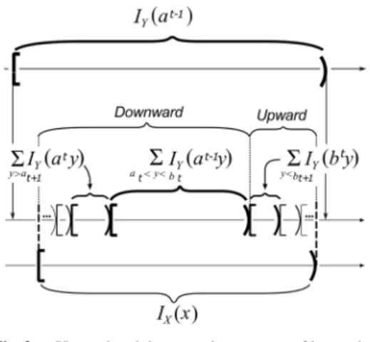
Fig. 3 Upward and downward sequences of intervals.

+ X

k≥t+1









 X

y>a_k

IY(a^k−1y)+X

y<bk

IY(b^k−1y)











. (16)

Proof of the equality (15) in Theorem 1 is quite parallel with that of the similar equality with respect top_X(x),x∈ X in[6]. For the equality (16) in Theorem 1, we give a simple and rigorous proof of this equality without depending on the equality (15). Lemma 1 is a key result for the proof. This lemma together with some simple observations on the p_Y- representations of two endpointsLX(x) andUX(x) ofIX(x), x∈ Xyields (16). The detail of the proof of Theorem 1 is given in Sect. 5.

It can be seen from the above presentation that the in- tervalP

a_t<y<b_tIY(a^t−1y) is in the middle of the intervalIX(x)

and that the sequence of intervals{P

y>a_k+1 I_Y(a^ky)}k≥t en-

tirely covers the lower part of the intervalIX(x). Those intervals are called downward sequencesin Han and Hoshi [3]. We also know that the sequence of intervals {P

y<b_k

I_Y(b^k−1y)}_k≥t₊₁in the third term in the right member of the above equation entirely covers the upper part ofIX(x). This sequence of the intervals are calledupward sequencein Han and Hoshi[3]. The result of Theorem 1 can be regarded as giving an explicit form of upward/downward sequences of intervals in the interval algorithm. Those sequences of intervals is shown in Fig. 3.

Based on the expression ofpX(x),x∈ Xin Theorem 1, set

D_t,x:=n

y^t:y^t−1=a^t−1,at< y_t<bt

o. (17) Furthermore, forl≥t+1, set

D_l,x:=n

y^l:y^l−1=a^l−1,al< y_lo

, (18)

U_l,x:=n

y^l:y^t−1=a^t−1, y_t^l−1=b^l−1_t , y_l<b_lo

. (19)

Then, we have the following.

S =X

x∈X











D_t,x+X

l≥t+1

D_l,x+X

l≥t+1

U_l,x











. (20)

Forx∈ X, define

D_x:=D_t,x+X

l≥t+1

D_l,x, U_x:= X

l≥t+1

U_l,x.

It is obvious thatS_x=D_x+U_x,x∈ X. In the remaining part of this section we present two examples of random number generation. For each example, we computeS_x,D_x, andU_x forx∈ X.

Example 3: We consider the case where M = 3, N = 4.

The target random variableXhas the following distribution:

pX =(pX(0),pX(1),pX(2),pX(3))

=(4/35,19/35,68/525, /16/75).

We assume that the stationary Markov process{Y_t}_t₌₁ specified with (11) in Example 1 generates coin random sequences. The p_Y-array representation for this example is discussed in Example 1. In the random number generation problem treated here the choice of pX is closely related to the periodic point of the mapτY defining the Markov shift.

In fact, we have LX(1) =4/35 =c1,LX(2) =23/35 =c2, LX(3)=59/75=c3, whereci,i=1,2,3 are the same quantity as those in Example 1. Those are the periodic points ofτY satisfyingτ²_Y(ci)=ci,i=1,2,3. Using the pY-array representations ofci,i=1,2,3 in Example 1, we have

LX(1)=0.02020202· · · , LX(2)=0.20202020· · · , LX(3)=0.21212121· · · .

Applying the formula (16) onIX(x),x∈ Xin Theorem 1 to the present example, we have the following:

IX(0)=X

k≥0

X

y<2

IY(0[20]^ky), IX(1)=IY(1)+X

k≥1

X

y>0

IY([02]^ky) +X

k≥1

X

y<2

IY([20]^ky), IX(2)=X

k≥0

X

y>0

IY(2[02]^ky)

+X

k≥1









 X

y<2

IY(2[12]^k1y)+IY(2[12]^k⁺¹0)









 , IX(3)=X

k≥0

IY(2[12]^k2).

Hence the setsS_x,D_x, andU_xforx=0,1,2,3 are S₀ =U₀=n

0[20]^k0,0[20]^k1o

k≥0, S₁ =D₁+U₁,











D₁ ={1}+n

[02]^k1,[02]^k2o

k≥1, U₁ =n

[20]^k0,[20]^k1o

k≥1, S₂ =D₂+U₂,









 D₂ =n

2[02]^k1,2[02]^k2o

k≥1, U₂ =n

2[12]^k10,2[12]^k11,2[12]^k⁺¹0o

k≥0,

(7)

S₃=D₃ =n

2[12]^k2o

k≥0.

Example 4: We consider the case where M = 3, N = 3.

The target random variableXhas the following distribution:

p_X =(p_X(0),p_X(1),p_X(2))=(1/7,40/63,2/9).

We assume that the stationary Markov process{Yt}_t₌₁specified with (13) in Example 2 generates coin random sequences. The pY-array representation for this example is discussed in Example 2. In the random number generation problem treated here the choice of pX is closely related to the periodic point of the mapτ_Y defining the Markov shift.

In fact, we have LX(1) = 1/7 = c⁰₁, LX(2) = 7/9 = c⁰₂, wherec⁰_i,i=1,2 are the same quantity as those in Example 2. Those are the periodic points ofτYsatisfyingτ²_Y(c⁰_i)=c⁰_i, i=1,2. Using thepY-array representations ofc⁰_i,i=1,2 in Example 2, we have

LX(1)=0.02020202· · ·, LX(2)=0.21212121· · ·. Applying the formula (16) onI_X(x),x∈ Xin Theorem 1 to the present example, we have the following:

IX(0)=X

k≥0

X

y<2

IY(0[20]^ky), IX(1)=IY(1)+X

k≥1

X

y>0

IY([02]^ky)

+X

k≥0











IY(2[12]^k0)+X

y<2

IY([21]^k⁺¹y)









 , I_X(2)=X

k≥0

I_Y(2[12]^k2).

Hence the setsS_x,D_x, andU_xforx=0,1,2 are S₀=U₀=n

0[20]^k0,0[20]^k1o

k≥0, S₁=D₁+U₁,











D₁={1}+n

[02]^k1,[02]^k2o

k≥1, U₁=n

2[12]^k0,[21]^k⁺¹0,[21]^k⁺¹1o

k≥0, S₂=D₂ =n

2[12]^k2o

k≥0.

4. Performance Analysis of the Interval Algorithm In this section we present a rigorous performance analysis of the interval algorithm using the expression of the interval algorithm we gave in the previous section.

4.1 Some Preliminaries

We define several quantities necessary for describing our result on the performance analysis of the interval algorithm.

LetS ∈S be a random variable with the distribution Prn

S =y^l∈ So

=pY(y₁)p_Y(y₂|y₁)· · ·pY(y_l|y_l−1).

Fory^l∈S define the mapϕ:S → Xsuch that

ϕ(y^l) :=xify^l∈ D_l,xory^l∈ U_l,x. (21) Defineϕ₁:S → {0,1}by

ϕ₁(y^l) :=(

0 ify^l∈ D_l,x

1 ify^l∈ U_l,x. (22)

SetV :=ϕ₁(S). Furthermore, define the mapϕ₂ :S → Y² by ϕ2(y^l) = (yl−1, yl). Set W := ϕ2(S). For each (a⁰,a)

∈ Y ×(Y − {0}), consider the set of integersl that satisfy y^l⁺¹ ∈ D_l₊_1,xand (yl, yl+1) =(a⁰,a).Letl1,a⁰,a,l2,a⁰,a,· · · be its elements arranged in the increasing order. By definition it is obvious that

t−1≤l1,a⁰,a<l2,a⁰,a<· · ·<lk,a⁰,a<lk+1,a⁰,a<· · ·. Similarly, for each (b⁰,b)∈ Y ×(Y − {M −1}), consider the set of integerslsatisfyingy^l⁺¹ ∈ U_l₊_1,xand (yl, yl+1) = (b⁰,b).Let ˜l_1,b⁰_,b,l˜_2,b⁰_,b,· · · be its elements arranged in the increasing order. By definition it is obvious that

t≤l˜_1,b⁰_,b<l˜_2,b⁰_,b<· · ·<l˜_k,b⁰_,b<l˜_k₊_1,b⁰_,b<· · · . Let

pS|VW X(y^l^k,a⁰^,a⁺¹|0,a⁰,a,x),k=1,2,· · ·,

denote conditional probabilities of S =y^l^k,a⁰^,a⁺¹ for given V = 0,W = (a⁰,a), andX = x. Let pS|VW X(·|0,a⁰,a,x) denote the probability distribution which consists of those probabilities. Similarly, let

pS|VW X(y^l^˜^k,b⁰^,b⁺¹|1,b⁰,b,x),k=1,2,· · ·,

denote conditional probabilities of S =y^l^˜^k,b⁰^,b⁺¹ for given V = 1,W = (b⁰,b), andX = x. Let pS|VW X(·|1,b⁰,b,x) denote the probability distribution which consists of those probabilities. In the remaining part of this subsection we compute the above two probability distributions, which will be useful for later arguments on the performance analysis of the interval algorithm. By the expression ofpX(x) using the coin random sequences we obtain

Prn

S =y^l^k,a⁰^,a⁺¹,V=0,W=(a⁰,a),X=xo

=Prn

Y^t−1=a^t−1,Y_t^l^k,a⁰^,a+1=a^l_t^k,a⁰^,aao

=pY(a^l_t^k,a⁰^,aa|a^t−1)pY(a^t−1)

(a)= pY(a^l_t^k,a⁰^,aa|at−1)p_Y(a^t−1), (23) where ifl1,a⁰,a =t−1, we definea^l_t^1,a⁰^,a =λ. Step (a) follows from the Markov property of coin random sequences.

Similarly, we obtain Prn

S =y^l^˜^k,b⁰^,b⁺¹,V=1,W=(b⁰,b),X=xo

=pY(b_t^l^˜^k,b⁰^,bb|at−1)pY(a^t−1). (24) Set

(8)

1332

η₀(a⁰,a,x|at−1) :=X

k≥1

pY(a^l_t^k,a⁰^,aa|at−1), (25) η1(b⁰,b,x|at−1) :=X

k≥1

pY(b^l_t^˜^k,b⁰^,bb|at−1). (26) From (23) and (25), we have

PrV=0,W=(a⁰,a),X=x =X

k≥1

1

×Prn

S =y^l^k,a⁰^,a⁺¹,V=0,W=(a⁰,a),X=xo

=X

k≥1

pY(a^l_t^k,a⁰^,aa|at−1)pY(a^t−1)

=η₀(a⁰,a,x|at−1)p_Y(a^t−1). (27) Similarly, from (24), and (26), we have

Pr

V=1,W=(b⁰,b),X=x

=η1(b⁰,b,x|at−1)pY(a^t−1). (28) From (23) and (24), we have

pS|VW X(y^l^k,a⁰^,a⁺¹|0,a⁰,a,x)

=Prn

S =y^l^k,a⁰^,a⁺¹

V =0,W =(a⁰,a),X=xo

= p_Y(a^l_t^k,a⁰^,aa|at−1)

η0(a⁰,a,x|at−1). (29)

Similarly, from (24) and (28), we have pS|VW X(y^˜^l^k,b⁰^,b⁺¹|1,b⁰,b,x)

= pY(b^˜^l_t^k,b⁰^,bb|at−1)

η₁(b⁰,b,x|a_t−1). (30)

Define two probability distributions on positive integers by p⁽⁰⁾_Y (·|a⁰,a,x,at−1)

:=

p_Y(a^l_t^k,a⁰^,aa|a_t−1)/η₀(a⁰,a,x|a_t−1)

k=1,2,···, p⁽¹⁾_Y (·|b⁰,b,x,at−1)

:=

pY(b^˜^l_t^k,b⁰^,bb|at−1)/η1(b⁰,b,x|at−1)

k=1,2,···. Then we have

pS|VW X(·|0,a⁰,a,x)=p⁽⁰⁾_Y (·|a⁰,a,x,at−1), (31) p_S_{|VW X}(·|1,b⁰,b,x)=p⁽¹⁾_Y (·|b⁰,b,x,a_t−1). (32) 4.2 Performance Evaluation of the Interval Algorithm In this subsection we state our main result on the performance analysis of the interval algorithm. In the following arguments,H(·) designates the entropy of a probability distribution or a random variable andD(·||·) designates the Kullback-Leibler divergence between two probability distributions.

For eachi∈ Y, letY2(i) be a random variable with the

distribution{P_{i j}}^M−1_j₌₀ . Entropy rate of{Y_t}^∞_t₌₁ is the following:

H(Y2|Y1)=

M−1

X

i=0

pY(i)

M−1

X

j=0

Pi j[−logPi j]

=

M−1

X

i=0

p_Y(i)H(Y₂(i)).

Define

Hmin(Y2(·)) := min

0≤i≤M−1H(Y2(i)), (33)

Hmax(Y2(·)) := max

0≤i≤M−1H(Y2(i)). (34)

Then we have

H_min(Y₂(·))≤H(Y₂|Y₁)≤H_max(Y₂(·)).

Here we have a certain nontrivial class of information sources where the above two bounds Hmin(Y2(·)) and Hmax(Y2(·)) match. For givenY1 = y1 ∈ Y, we define a probability distributionQy₁by

Qy₁ :=pY(·|y1)={Py₁y₂}_y₂_∈Y

LetS(Y) denote the representation of the symmetric group of permutations ofYby the|Y| × |Y|permutation matrix.

We consider the following condition.

Condition:We call that the stochastic matrixPsatisfies a symmetrical property if for any y₁, y⁰₁ ∈ Y, there exists Π∈S(Y) such thatQy⁰₁=Qy₁Π.

Then we have the following.

Lemma 2: If the stochastic matrix P of the stationary Markov information source{Yt}_t₌_1,2,···satisfies a symmetrical property, we have

Hmin(Y2(·))=H(Y2|Y1)=Hmax(Y2(·)).

Proof: Letimin ∈ Y be the symbol i such that it at- tainsH_min(Y₂(·)) defined by (33). Similarly, leti_max ∈ Ybe the symbolisuch that it attainsHmax(Y2(·)) defined by (34).

SincePsatisfies a symmetrical property, we have that Qimin =QimaxΠ for someΠ∈S(Y). (35) Then we have the following chain of equalities:

Hmin(Y2(·))=H(Qi_min)^(a)=H(Qi_maxΠ)^(b)=H(Qi_max)

=Hmax(Y2(·)).

Step (a) follows from (35). Step (b) follows from that the entropy is invariant under the permutation on the components

of the probability vectorQimax.

In the following we show three examples ofPwith a symmetrical property.

Example 5: We consider the case where M = 3. Set θi := P0i,i = 0,1,2. The following three stochastic ma- tricesPi,i=1,2,3 are examples ofPhaving a symmetrical

(9)

property.

P₁=





 θ₀θ₁θ₂ θ0θ1θ2

θ₀θ₁θ₂





 ,P₂=





 θ₀θ₁θ₂ θ1θ2θ0

θ₂θ₀θ₁





 ,P₃=





 θ₀ θ₁θ₂ θ0 θ2θ1

θ₀ θ₁θ₂





 . The above three examples have some specific properties.

WhenP = P1, the source becomes the stationary memoryless source specified with pY = (pY(0),pY(1),pY(2)) = (θ0, θ1, θ2). P2 is a doubly stochastic matrix. When we chooseθ0 =θ1 =0.25,θ2 =0.50 inP3,P =P3coincides with the stochastic matrix in Example 2.

The efficiency of the interval algorithm is measured by the average number of coin tosses necessary to obtain the target random variable. We denote it by ¯L. According to Han and Hoshi[3], we have the following:

Lemma 3(Han and Hoshi[3]):

LH¯ min(Y2(·))≤H(S)≤LH¯ max(Y2(·)).

Specifically, if the stochastic matrix P of the stationary Markov information source{Y_t}_t₌_1,2,···satisfies a symmetrical property, we have ¯LH(Y2|Y1)=H(S).

From this lemma we can see that an evaluation of ¯Lis reduced to an estimation of upper bound of H(S). On the upper bound of this quantity, we have the following lemma.

Lemma 4:

H(S)≤H(X)+log{2M(M−1)}+ζ, (36) whereζ:=H(S|VW X). For the quantityζ, we have

ζ=

N−1

X

x=0

pY(a^t(x)−1)











M−1

X

a⁰=0 M−2

X

a=0

η0(a⁰,a,x|at−1)

×H

p⁽⁰⁾_Y (·|a⁰,a,x,a_t−1) +

M−1

X

b⁰=0 M−1

X

b=1

η1(b⁰,b,x|at−1)

×H

p⁽¹⁾_Y (·|b⁰,b,x,at−1)

. (37)

Proof:We first prove (36). We have the following:

H(S)=H(ϕ(S)ϕ1(S)ϕ2(S)S)=H(XVWS)

=H(X)+H(VW|X)+H(S|VW X)

≤H(X)+log{2M(M−1)}+H(S|VW X),

where the last inequality follows from thatVis a binary random variable and thatW takes values inY ×(Y − {M−1}) ifV =1 and takes values inY ×(Y − {0}) ifV =0. From (27), (28), (31), and (32), we have (37).

Han and Hoshi[3]used several complicated arguments to derive the upper bound ofH(S|VW X). Their result is the following.

Theorem A(Han and Hoshi[3]):

H(X)

Hmax(Y2(·)) ≤L¯ ≤ H(X)

Hmin(Y2(·))+log{2M(M−1)}

Hmin(Y2(·)) + h(p_max)

(1−p_max)Hmin(Y2(·)), (38) where

p_max:= max

(y₁,y₂)∈Y²

P_y₁_y₂

andh(·) is the binary entropy function.

Define the geometrical distribution p^∗ with parameter p_maxby

p^∗:=

p_max^k−1(1−p_max)

k=1,2,···

Our main result on the performance analysis of the interval algorithm is the following.

Theorem 2:

H(X)

Hmax(Y₂(·)) ≤L¯ ≤ H(X)

Hmin(Y₂(·))+log{2M(M−1)}

Hmin(Y₂(·)) + h(p_max)

(1−p_max)Hmin(Y2(·))− ∆

Hmin(Y2(·)), (39) where∆is a nonnegative number defined by

∆ =

N−1

X

x=0

pY(a^t(x)−1)











M−1

X

a⁰=0 M−1

X

a=1

η₀(a⁰,a,x|at−1)

×D

p⁽⁰⁾_Y (·|a⁰,a,x,at−1) p^∗ +

M−1

X

b⁰=0 M−2

X

b=0

η1(b⁰,b,x|at−1)

×D

p⁽¹⁾_Y (·|b⁰,b,x,at−1) p^∗

. (40)

Specifically, if the stochastic matrix P of the stationary Markov information source{Yt}_t₌_1,2,···satisfies a symmetrical property, we have

H(X)

H(Y₂|Y1) ≤L¯≤ H(X)

H(Y₂|Y1)+log{2M(M−1)}

H(Y₂|Y1) + h(p_max)

(1−p_max)H(Y2|Y1)− ∆

H(Y2|Y1). (41) Proof of Theorem 2 is given in the next section. Let the upper bound of ¯Lby Han and Hoshi[3]in (38) be denoted by ¯LHH. Then our upper bound of ¯Lin Theorem 2 is

L¯≤L¯HH− ∆

H_min(Y₂(·)). (42)

Note that∆is nonnegative and may almost always be positive. Hence our upper bound improves ¯LHH. The bound (42) is equivalent to ¯L_HH−L¯ ≥∆/H_min(Y₂(·)), implying that the quantity ∆/Hmin(Y2(·)) serves as a lower bound on the deviation of ¯LHHfrom the true value of ¯L.

Remark:In[7], the author made a mistake in the derivation of the upper bound of ¯L. Hence the upper bound of ¯Lgiven