Parameter Estimation of Fractional Bandlimited LFM Signals Based on Orthogonal Matching Pursuit

(1)

PAPER

Parameter Estimation of Fractional Bandlimited LFM Signals Based on Orthogonal Matching Pursuit

Xiaomin LI^†,††a),Nonmember, Huali WANG^†††b),Member,andZhangkai LUO^{††††c)},Student Member

SUMMARY Parameter estimation theorems for LFM signals have been developed due to the advantages of fractional Fourier transform (FrFT).

The traditional estimation methods in the fractional Fourier domain (FrFD) are almost based on two-dimensional search which have the contradiction between estimation performance and complexity. In order to solve this problem, we introduce the orthogonal matching pursuit (OMP) into the FrFD, propose a modified optimization method to estimate initial frequency and final frequency of fractional bandlimited LFM signals. In this algorithm, the differentiation fractional spectrum which is used to form observation matrix in OMP is derived from the spectrum analytical formulations of the LFM signal, and then, based on that the LFM signal has approximate rectangular spectrum in the FrFD and the correlation between the LFM signal and observation matrix yields a maximal value at the edge of the spectrum (see Sect. 3.3 for details), the edge spectrum information can be extracted by OMP. Finally, the estimations of initial frequency and final frequency are obtained through multiplying the edge information by the sampling frequency resolution. The proposed method avoids reconstruction and the traditional peak-searching procedure, and the iterations are needed only twice. Thus, the computational complexity is much lower than that of the existing methods. Meanwhile, Since the vectors at the initial frequency and final frequency points both have larger modulus, so that the estimations are closer to the actual values, better normalized root mean squared error (NRMSE) performance can be achieved. Both theoretical analysis and simulation results demonstrate that the proposed algorithm bears a relatively low complexity and its estimation precision is higher than search-based and reconstruction-based algorithms.

key words: linear frequency modulation signal, parameter estimation, orthogonal matching pursuit, fractional Fourier transform

1. Introduction

Fractional Fourier transform (FrFT) is a powerful tool for analyzing LFM signals which are also known as chirp signals[1]. FrFT uses a transform kernel which essentially allows the signal in the time-frequency domain to be projected onto a line of arbitrary angle. The definition of FrFT is denoted by[2]:

Manuscript received May 15, 2019.

†The author is with School of Electronic and Optical Engi- neering, Nanjing University of Science and Technology, Nanjing 210094, China.

††The author is with School of Mechanical and Electrical En- gineering, Henan Institute of Science and Technology, Xinxiang 453003, China.

†††The author is with College of Communication Engineer- ing, The Army Engineering University of PLA, Nanjing 210007, China.

††††The author is with Science and Technology on Complex Elec- tronic System Simulation Laboratory, Space Engineering Univer- sity, Beijing 101416, China.

a) E-mail: [email protected]

b) E-mail: [email protected] (Corresponding author) c) E-mail: luo [email protected]

DOI: 10.1587/transfun.E102.A.1448

Xp(u)=n

Fp[x(t)]o

(u)=R∞

−∞x(t)Kp(t,u)dt (1) WhereF_pdenotes the FrFT operator. The kernel function is denoted by:

Kp(t,u)=











Aαexpjπh t²+u²

cotα−2utcscαi

, α,nπ

δ(t−u), α=nπ

δ(t+u), α=(2n+1)π

(2)

Where Aα = p

1−jcotα, and α = ^pπ₂ is the transform angle. FrFT can be interpreted as a signal decompo- sition in terms of a chirp basis as its kernel is constituted by chirp functions, so FrFT has a notable potential for analyzing chirp signals[1],[3]. For the LFM signal detection and parameter estimation, FrFT is densely used by making use of the change of the concentration, or equivalently the support. In the fractional Fourier domain (FrFD), support of LFM signals change associated with the transform angle and there exists an optimum transform angle in which the energy of chirp signals are most concentrated[4],[5].

when an LFM signal is transformed by FrFT at its optimum angle, transform kernel acts as a matched filter. Therefore, an optimum LFM detection and estimation can be done by sweeping all of the angles and finding the correct angle that maximizes the absolute amplitude. Almost all successful methods employing FrFT use the maximum peak of sweep in the FrFD[4],[6]–[11], which is an easy method to realize.

And obviously, the search-based algorithms above require numerous extra calculations and have the contradiction between estimation performance and complexity.

In recent years, numerous researchers have explored the parameter estimation problem of chirp signals from different aspects[1],[9],[12]–[22]. Inspired by the recently- developed sparse reconstruction method[23]–[28], we propose a fast and high accuracy parameter estimation method for LFM signals in the FrFD based on orthogonal matching pursuit (OMP). In this algorithm, We construct the observation matrix through the differentiation spectrum, and prove that the LFM signal and observation matrix are most rele- vant at the edge of the fractional spectrum, so the fractional spectrum edge information can be extracted by OMP. And the estimations of initial frequency and final frequency can be gotten through multiplying the sampling frequency resolution by the edge information.

Neither reconstruction nor peak-searching are needed in the proposed method, which can reduce the computa- Copyright c2019 The Institute of Electronics, Information and Communication Engineers

(2)

tional complexity greatly. And the estimation precision is higher than existing algorithms because of the larger modulus the vectors at the initial frequency and final frequency points have (see Sect. 3.3 for details). Simulation results demonstrate that the proposed algorithm has better normalized root mean squared error (NRMSE) performance.

The remainder of this paper is organized as follows: In Sect. 2, the basic preliminaries is presented. The new algorithm is proposed in Sect. 3. In Sect. 4, the parameters estimation performance is simulated and analyzed. Section 5 is the conclusion.

2. Preliminaries

2.1 Simplified Fractional Fourier Transform (SFrFT) FrFT is an extension of the ordinary Fourier transform (FT), which essentially allows the signal in the time-frequency domain to be projected onto a line of arbitrary angle[29].

Simplified fractional Fourier transform (SFrFT)[30]has the same effect as FrFT of orderαfor filter design, but it is sim- pler to implement digitally than the original FrFT. And the first type ofαth-order SFRFT is defined as[30]:

Yα(u)=(j2π)⁻¹²

×R∞

−∞exp

−jut+jt²cotα/2 y(t)dt

(3) whereαis the SFrFT order. The inverse SFrFT is denoted as follows:

y(t)=(j/2π)¹²exp

−ju²cotα/2

×R∞

−∞exp (jut)Yα(u)dt

(4) The digital implementation of SFrFT (DSFrFT) is given by [30]

Fα[m]=(j2π)⁻¹²∆t

N

X

n=−N

exp −j 2πmn 2N+1+ j

2n²cotα(∆t)²

!

·y[n]

(5)

Wherey[n] = y[n∆t], Fα[m] = Fα[m∆u],m, n = −N,

−N+1,N,∆tand∆u are the sample spacing in temporal domain and simplified fractional Fourier domain (SFrFD) respectively. And∆t∆u =2π/(2N+1). We can also write (5) in matrix form, expressed as

Fα=c1O^α_Fy

Wherec1 = (j2π)⁻¹²∆t, O^α_F−1

= O^α_F∗

, ∗ denotes the transposed conjugate operator, andO^α_F is a (2N+1)× (2N+1) unitary matrix whose elementh

O^α_Fi

mnat themrow, ncolumn has the following form:

O^α_F

mn =expl

−j2π(m−N−1)(n−N−1) 2N+1

m

·expl

j(n−N−1)²cotα(∆t)²/2m

whered·ereturns the nearest integer towards positive infin- ity. With the change ofα, the frequency axis of the SFrFT is located in different positions, and more abundant information about the frequency characteristics of the signal can be obtained compared to the FT.

2.2 Fractional Bandlimited LFM Signal and Its Spectral Features in SFrFD

A fractional bandlimited LFM signal f(t) has finite energy. The SFrFT of f(t) is zero outside the region (−u₀−u_α,−u₀+u_α)∪(u₀−u_α,u₀+u_α).

i.e.

Fα(u)=











Fα(u),u0−uα≤ |u| ≤u0+uα

0, otherwise (6)

Where 2uαis the fractional bandwidth of f(t). Accord- ing to Parseval’s theorem, the bandlimited LFM signal can also be expressed as:

R∞

−∞|f(t)|²dt=R−u_l

−uh |Fα(u)|²du+Ru_h

ul |F_α(u)|²du whereuh=u0+u_α, andul=u0−u_α.

The LFM signal model is given by x(t)=A·exp

j2πf0t+ jπKl f mt²

(7) Where f0is the initial frequency,Ais the amplitude ofx(t) which could be random or fixed.K_{l f m}is the modulation rate.

And using the results in Appendix, for the LFM signal whose duration time ish

−^T₂^d,^T₂^di , when

K_{l f m}+cotα/2π T_d² 1, its amplitude spectrum in SFrFD is

|X_α(u)|

≈ 1

pKl f m+cotα/2π·rect u−2πu₀cscα B⁰

! (8)

and its phase spectrum in SFrFD is θ(u)≈ −π(u−2πu0cscα)²

Kl f m+cotα/2π +π

4 (9)

Where B⁰ is the width of the spectrum in SFrFD, K_{l f m}⁰ = K_{l f m}+cotα/2π, andαis the fractional orders. And according to (6) and (8), the LFM signalx(t) whose duration time ish

−^T₂^d,^T₂^di

is a fractional bandlimited signal.

3. Proposed Parameter Estimation Method for Frac- tional Bandlimited LFM Signals

3.1 Method Description

In this part, we propose an optimization method to estimate initial frequency and final frequency of fractional bandlimited LFM signals by introducing the OMP. The proposed method is based on two principles. First, the LFM signal has a rectangular spectrum in the SFrFD ofα-th order when

(3)

T_d·p

|K_{l f m}+cotα| 1 (see Appendix for details), and the correlation between the LFM signal and observation matrix yields a maximal value at the edge of the fractional spectrum (see Sect. 3.3 for details). Second, OMP algorithm have the ability to search the maximum correlation information.

In the proposed method, the differentiation spectrum which is used to form the observation matrix is derived from the spectrum analytical formulations of the LFM signal in the FrFD, and then the correlation between the LFM signal and observation matrix is proved to be the largest at the edge of the fractional spectrum, as a result, the spectrum edge information can be extracted by OMP. Finally, multiply the sampling frequency resolution by the edge information to get the estimations of initial frequency and final frequency.

There are only two iterations in the method, neither reconstruction nor the traditional peak-searching procedures are needed, thus, the computational complexity is much lower than the existing methods. Meanwhile, since the vectors at the initial frequency and final frequency points both have larger amplitude, so that better NRMSE performance can be achieved as well.

3.2 The Differential Procedure for the Fractional Spec- trum of the LFM Signal

The fractional bandlimited LFM signals can be depicted as y_m=A·e^j[^2π(ⁿln/K+K_{l f m}n²/2K²)]^|n=0,1,···,K−1

=A·e^j

2π

nl K

n−ⁿ_2K²

+^nhKn2 2K

|_n₌0,1,···,K−1

=ym(0) ym(1) · · · ym(K−1)T

(10)

wherenl is the initial frequency point, nh is the final frequency point. K_{l f m} is the modulation rate. Kis the number of sampling data.

The DSFrFT ofy_mis[30]

Fα=c1O^α_Fym

the differentiating process forFαcan be expressed as y= Γ⁰·Fα= Γ⁰·c1O^α_Fy_m (11)

whereΓ⁰=







1 −1 · · · 0

0 1 ... 0

0 ... ... −1

0 · · · 0 1







K×K

is the differentiating matrix.c1=(j2π)^−1/2∆t,

O^α_F =







O^α_F(1,1) O^α_F(1,2) · · · O^α_F(1,K) O^α_F(2,1) O^α_F(2,2) · · · O^α_F(2,K)

... ... ... ...

O^α_F(K,1) O^α_F(K,2) · · · O^α_F(K,K)







K×K

is the DSFrFT matrix, andO^α_F is unitary matrix. The ele- ments of matrixO^α_F are:

O^α_F(m,n)=expl

−j^2π(m−N_2N⁰^−1)(n−N0+1 ⁰⁻¹⁾

m

·expl

j n−N⁰−12

cotα(∆t)²/2m m,n=1,· · ·,N⁰,· · ·,K,N⁰=l_K−1

2

m,∆t= ¹_f_s From Eq. (11),

y_m= Γ⁰·c1O^α_F⁻¹·y=G⁰·y (12) Where

G⁰= Γ⁰·c1O^α_F−1=(j/2π)^1/2/(K∆t)·







1

P

n=1

O^α_F(1,n)

2

P

n=1

O^α_F(1,n) · · ·

k

P

n=1

O^α_F(1,n)

1

P

n=1

O^α_F(2,n)

2

P

n=1

O^α_F(2,n) · · ·

k

P

n=1

O^α_F(2,n)

... ... ... ...

1

P

n=1

O^α_F(K,n)

2

P

n=1

O^α_F(K,n) · · ·

k

P

n=1

O^α_F(K,n)







∗

K×K

3.3 The Correlation betweenG⁰andy_m

Assume the initial residual res0 = ym, observation matrix G⁰ =

Γ⁰·c1O^α_F−1

, so the correlation betweenres0 andG⁰ can be computed according to their inner product as follows:

|res0,G⁰|=(j/2π)^1/2/(K∆t)·







|

1

P

n=1

O^α_F(n,1)ym(1)+· · ·+P¹

n=1

O^α_F(n,k)ym(k)|

|

2

P

n=1

O^α_F(n,1)ym(1)+· · ·+P²

n=1

O^α_F(n,k)ym(k)| ...

|

K

P

n=1

O^α_F(n,1)ym(1)+· · ·+P^K

n=1

O^α_F(n,k)ym(k)|







K×1

(13) Whereh·idenotes the inner product operator. Since the DS- FrFT ofym(n) is

Fα(m)=c1 K

P

n=1

O^α_F(m,n)·ym(n) Equation (13) can be reduced to:

|res0,G⁰|

=|res0, g⁰₁||res0, g⁰₂| · · · |res0, g⁰_K|T

=(j/2π)^1/2/(K∆t)·







|Fα(1)|

|F_α(1)+F_α(2)| ...

|Fα(1)+Fα(2)+· · ·+Fα(k−1)|

|Fα(1)+Fα(2)+· · ·+Fα(k−1)+Fα(k)|







K×1

=(j/2π)^1/2/(K∆t)·







|

1

X

m=1

Fα(m)||

2

X

m=1

Fα(m)| · · · |

K

X

m=1

Fα(m)|







T

(14)

(4)

According to (14), |D

res0, g⁰_kE

|, the kth element of

| hres0,G⁰i |, denotes the summation of the firstkterms from F_α(m), which is the DSFrFT ofy_m(n). And for the LFM signalym, whenTd·p

|Kl f m+cotα| 1, its amplitude spectrum and phase spectrum inα-th order discrete time simplified fractional Fourier domain (DTSFrFD) are respectively:

|X_α(u)|

≈ A

pKl f m+cotα·rect u−2πu₀cscα B⁰

! (15)

θ(u)≈π(u−2πu0cscα)² Kl f m+cotα +π

4 (16)

Substitute (15) and (16) into(14),

|D res0, g⁰_kE

|=











0, k<nl

|⁽^j/2π)

1 2

K∆t · √ ^A

K_{l f m}+cotα·

k−n_l

P

m=1

e^jφ(m)|, nl≤k≤nh

|⁽^j/2π)

12

K∆t · √ ^A

K_{l f m}+cotα·

k−n_l

P

m=1

e^jφ(m)|, k>nh

(17)

Whereφ(m)=−_K^π(m^∆⁾²

l f m+cotα+^π₄, 0≤m≤nh−nl, and

∆φ(m)=φ(m)−φ(m+1)=π(2m+1)∆²

K_{l f m}+cotα (18) whennl≤k≤nh,|D

res0, g⁰_kE

|can be expressed as the sum of ⁽^j/2π)

1 2

K∆t · √ ^A

K_{l f m}+cotα ·e^jφ(m), whose phase changes nonlin-

early in Eq. (18) as Fig. 1.

Let vectorB = ⁽^j/2π)_K_∆_t¹² · √ ^A

Kl f m+cotα ·e^jφ(m). And Fig. 1

also shows that vector B with constant magnitude, moves clockwise on a circle. Meanwhile, φ(m), the phase of B, increases with an interval of∆φ(m), therefore|D

res0, g⁰_kE

| will increase at first and then decrease. According to (18),

∆φ(m) increases asBmoves along the circle clockwise, the

Fig. 1 The vector B with constant magnitude.

accumulated phase energy of|D

res0, g⁰_kE

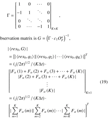
|reaches its maximum value within the first cycle. And this maximum value is corresponding to the estimation of initial frequency. Sim- ilarly, when differentiating matrix is

Γ =







1 0 · · · 0

−1 1 ... 0

0 ... ... 0

0 · · · −1 1







K×K

,

observation matrix isG=

Γ·c1O^α_F−1

,

| hres0,Gi |

=| hres0, g1i || hres0, g2i | · · · | hres0, g_Ki |T

=(j/2π)^1/2/(K∆t)·







|F_α(1)+F_α(2)+F_α(3)+· · ·+F_α(K)|

|Fα(2)+Fα(3)+· · ·+Fα(K)| ...

|Fα(K)|







K×1

=(j/2π)^1/2/(K∆t)·







|

K

X

m=1

Fα(m)||

K

X

m=2

Fα(m)| · · · |

K

X

m=K

Fα(m)|







T

(19)

And a similar analysis can be perform for| hres₀, gki |, as a result, the maximum value of| hres0, gki |is corresponding to the estimation of final frequency.

3.4 The Parameter Estimation Procedures Using OMP Assume res0 is the residual, i is the iteration count, Λ0

is a set of indices of the nonzero channel coefficients.

g⁰_k(k=1,2,· · ·,K) is the columns of observation matrixG⁰. Andym=G⁰·y. Accordingly, the initial frequency estimation procedures of the proposed method is summarized in Algorithm 1.

Algorithm 1: the initial frequency estimation (1) Initializeres₀=ym,i=1 andΛ0=∅.

(2) Determine the new indexλ⁰_iby selecting the maximum absolute value of the correlation betweenG⁰and previous residualres₀. That is,λ⁰_i=arg max

k=1,2,···,N/2|D res_i−1, g⁰_kE

|.

(3)combine the newly selected indexλ⁰_iwith the indexΛi−1, i.e., Λi= Λi−1∪n

λ⁰_io . Compute theyi=arg min_y

ym−G⁰_Λ

iy ₂. Compute the new residualres_i=ym−G⁰_Λ

iyi. (4) Seti=i+1 ifi<3 go to step 2.

The stopping criterion in Algorithm 1 isi =3, which means that two iterations fory_m =G⁰·yis required. As a result,λ⁰₁andλ⁰₂, the index which are corresponding to the maximum values of the correlation betweenG⁰and residual

(5)

Fig. 2 The relationship between |D res_i−1, g⁰_kE

|and the fractional “frequency”.

within each iterations, are obtained. And the estimated initial frequency of LFM signal in DTSFrFD is min

λ⁰₁, λ⁰₂

∆, where∆ =1/KT_s,Tsis the sampling interval.

Similarly, when observation matrix isG=

Γ·c1O^α_F−1

, conduct two iterations ony_m=G·yto generate two indexs λ1,λ2. Then the estimated final frequency in DTSFrFD is max (λ₁, λ₂)∆, where∆ =1/KT_s. Figure 2 illustrates the relationship between|D

resi−1, g⁰_kE

|,i=1,2 and the fractional

“frequency”. Figure 2(a) shows that there are two maximum values atnlandnhrespectively after the first iteration. Thus the indexλ⁰₁ corresponds to eithernlornh. Compared with Fig. 2(a),|D

res1, g⁰_kE

|has a smaller value atnh as shown in Fig. 2(b), because the update process in OMP removes the influence ofgλ⁰₁ from|D

res0, g⁰_kE

|. Accordingly, the maximum value obtained by the second iteration is the second largest value of|D

res0, g⁰_kE

|, i.e., the value corresponding to n_l. Since the LFM signal has approximate rectangular spectrum in DTSFrFD, so whenk>nh,Fα(m) is approximately zero, which leads to an almost constant value of|D

res₀, g⁰_kE

|, as shown in Fig. 2(a). Therefore, after two iterations, the index min

λ⁰₁, λ⁰₂

corresponds ton_l, which is the initial frequency.

Similarly, Fig. 3 illustrates the relationship between

| hresi−1, gki |i = 1,2 and the fractional “frequency”. And after two iterations, the index max (λ₁, λ₂) is corresponding tonhwhich is the final frequency.

Thus, the estimated initial frequency is

f0=u0·cscα=min λ⁰₁, λ⁰₂∆·cscα (20) the final frequency estimated is

f1=u1·cscα=[max (λ1, λ2)∆]·cscα (21) 3.5 Influence of the Fractional Order

According to the analysis above, algorithm 1 can effectively

Fig. 3 The relationship between| hres_i−1, g_ki |, and the fractional “frequency”.

extract the edge information of the spectrum in DTSFrFD.

Since theαth-order SFrFT can be regarded as the projection on the rotated frequency axisu, so the spectrum distribution of the signal directly depends on the order of the SFrFT. Ac- cording to the analysis in Appendix, for a discrete-time LFM signal with the duration ofh

−^T^d

2,^T₂^di

, its amplitude spectrum in DTSFrFD is

|X_α(u)| ≈ A

pKl f m+cotα·rect u−2πu0cscα B⁰

! ,

when

Kl f m+cotα/2π

T_d²1. WhereB⁰is the bandwidth of the spectrum,αis the fractional orders.

whenT_dandK_{l f m}are constant, the fluctuation of Fresnel integral decreases as cotαincreases. So the shape of|Xα(u)| is closer to rectangle and the edge feature of the spectrum is more distinct as shown in Fig. 4, which improves the effi- ciency of Algorithm 1.

4. Simulation and Analysis

4.1 Simulation Configurations

To evaluate the performance of the proposed method, a uni- formly sampled chirp signal is tested. The original chirp signal in discrete-time domain is denoted by x(n). The noisy signal is x(n)+w(n), wherew(n) is the zero-mean Gaus- sian noise. The SNR is defined by 10 log

kxk²/kwk . x(n) is given by x(n) = Ee^jπK^{l f m}ⁿ²^/f^{NY Q}² cos 2πfln/fNY Q, where Eis the amplitude of the signal which could be random or fixed. Kl f m=0.200×10⁹Hz/sis the signal modulation rate.

The Nyquist sampling rate is f_{NY Q}=u_{NY Q}cscα=2.2GHz, whereuNY Qis the sampling rate in FrFD.αis the bandlimited order which varies from−0.50×10⁻⁸to−0.36×10⁻⁸ with a step of −0.01×10⁻⁸. The signal duration time is T =1s. So the bandwidth ofx(n) isB=Kl f m·T =10MHz,

(6)

Fig. 4 The amplitude spectrums of the LFM signal in DTSFrFD with different orders(S NR=15dB).

fl = 1GHz is the initial frequency. The signal is both frequency bandlimited and fractional bandlimited with different bandwidths in the observation interval. Simulations were conducted to valid ate parameter estimation accuracy.

Each simulation has 300 trials to ensure statistically stable results.

4.2 Parameter Estimation Accuracy

In this experiment, we test the parameter estimation accuracy of our proposed method, compared with the tradi-

Fig. 5 The performance in the noise-free case.

tional search-based method [11] and reconstruction tech- nique[28]. The parameter estimation accuracy is evaluated by the NRMSE in the noise-free and noisy cases. And the NRMSE is defined as:

fNRMS E=

s

1 N

PN n=1

_

f_n−f_n 2

max _

f_n

−min _

f_n

WhereNis the number of Monte Carlo trials,

_

fnis the estimation signal frequency from then-th Monte Carlo experiment, fn is the original signal frequency. Figure 5 depicts the tradeoff between NRMSE and the fractional order α in the noise-free case. The orders α varies from

−0.50×10⁻⁸to−0.36×10⁻⁸with a step of−0.01×10⁻⁸. Ac- cording to the previous analysis, fractional orderαmay lead to changes in the spectral width. The wider the spectrum, the better estimation performance can be achieved. And it is observed that a smaller NRMSE correspond to largerαand vice versa.

In the noisy case, the simulations demonstrated two aspects:

the tradeoff between NRMSE and the fractional order α, and the balance between NRMSE and signal-to-noise ratio (SNR).

(7)

Fig. 6 The relationship between the NRMSE and ordersαin the noise case.

Figure 6 shows the relationship between the NRMSE and orders α. In Fig. 6, the SNR is {5,25}dB, the orders αvaries from−0.50×10⁻⁸ to−0.36×10⁻⁸with a step of

−0.01×10⁻⁸. The increase ofαleads to the wider bandwidth and the NRMSE decreases.

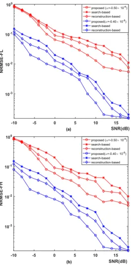
In Fig. 7, the SNR varies from−10dBto 18dBwith a step of 2 dB. The fractional orderαisn

−0.50×10⁻⁸,−0.40

×10⁻⁸o

. It is common that the NRMSE decreases with in- creasing SNR in both the proposed method and compared methods. And it is clear that the proposed method has better accuracy.

Figure 8 depicts the performance in terms of NRMSE with different SNRs and fractional orderαfor the proposed method. The SNR varies from−105dBto 18dBwith a step of 2dB. The fractional orderαvaries fromn

−0.50×10⁻⁸o ton

−0.36×10⁻⁸o

with a step ofn

−0.02×10⁻⁸o

. It is observed that the NRMSE has the opposite trend as the SNR.

5. Conclusion

This paper introduces a parameter estimation method to determine the initial frequency and final frequency of the fractional bandlimited LFM signals by using OMP. The edge

Fig. 7 The relationship between the NRMSE and SNR.

Fig. 8 The relationship between the NRMSE and SNR.

information of the spectrum can be extracted effectively in DTSFrFD, and the corresponding frequencies are obtained.

The proposed method avoids reconstruction and the traditional peak-searching procedure, and it only needs two iterations. The theoretical analysis and the simulations results

(8)

demonstrate better performance of the proposed method in comparison with existing methods.

Acknowledgments

This work is supported by National Natural Science Founda- tion of China (No. 61271354) and Henan Province Science and Technology Key Project (No. 142102210431).

References

[1] A. Serbes, “On the estimation of LFM signal parameters: Analyti- cal formulation,” IEEE Trans. Aerosp. Electron. Syst., vol.54, no.2, pp.848–860, 2018.

[2] H.M. Ozaktas, Z. Zalevsky, and M.A. Kutay, The Fractional Fourier Transform: With Applications in Optics and Signal Processing, Wi- ley, 2001.

[3] R. Tao, B. Deng, and Y. Wang, “Research progress of the fractional Fourier transform in signal processing,” Sci. China, vol.49, no.1, pp.1–25, 2006.

[4] L. Qi, R. Tao, S. Zhou, and Y. Wang, “Detection and parameter estimation of multicomponent LFM signal based on the fractional Fourier transform,” Sci. China Ser. F: Inf. Sci., vol.47, no.2, pp.184–

198, 2004.

[5] C. Capus and K. Brown, “Fractional Fourier transform of the Gaus- sian and fractional domain signal support,” IEE Proceedings - Vi- sion, Image and Signal Processing, vol.150, no.2, pp.99–106, 2003.

[6] Y. Zhao, Y. Hua, W. Gang, J.I. Fei, and F. Chen, “Parameter estimation of wideband underwater acoustic multipath channels based on fractional fourier transform,” IEEE Trans. Signal Process., vol.64, no.20, pp.5396–5408, 2016.

[7] X. Liu and C. Wang, “A novel parameter estimation of chirp signal inα-stable noise,” IEICE Electron. Express, vol.14, no.8, pp.1–11, 2017.

[8] Y. Liu, Y. Zhao, J. Zhu, Y. Xiong, and B. Tang, “Iterative high- accuracy parameter estimation of uncooperative OFDM-LFM radar signals based on FrFT and fractional autocorrelation interpolation,”

Sensors, vol.18, no.10, pp.3550–3559, 2018.

[9] L. Tao, Z. Qian, X. Fan, and P. Chen, “Parameter estimation of LFM signal intercepted by improved dual-channel Nyquist folding receiver,” Electron. Lett., vol.54, no.10, pp.659–661, 2018.

[10] J. Song, Y. Liu, and Y. Wang, “Iterative interpolation for parameter estimation of LFM signal based on fractional Fourier transform,”

Circuits Syst. Signal Process., vol.32, no.3, pp.1489–1499, 2013.

[11] Y. Chen, L. Guo, and Z. Gong, “The concise fractional Fourier transform and its application in detection and parameter estimation of the linear frequency-modulated signal,” Chinese J. Acoust., no.1, pp.70–86, 2017.

[12] Y.X. Zhang, R.J. Hong, C.F. Yang, Y.J. Zhang, Z.M. Deng, and S. Jin, “A fast motion parameters estimation method based on cross- correlation of adjacent echoes for wideband LFM radars,” Applied Sciences, vol.7, no.5, p.500, 2017.

[13] Y. Jin and D. GAO, “Parameter estimation of LFM signals based on synchrosqueezing chirplet transform in complicated noise,” J. Elec- tron. Inf. Technol., vol.39, no.8, pp.1906–1912, 2017.

[14] S. Barbarossa, “Analysis of multicomponent LFM signals by a combined Wigner-Hough transform,” IEEE Trans. Signal Process., vol.43, no.6, pp.1511–1515, 1995.

[15] G. Bai, Y. Cheng, W. Tang, and S. Li, “Chirp rate estimation for LFM signal by multiple DPT and weighted combination,” IEEE Sig- nal Process. Lett., vol.26, no.1, pp.149–153, 2019.

[16] F.G. Geroleo and M. Brandt-Pearce, “Detection and estimation of LFMCW radar signals,” IEEE Trans. Aerosp. Electron. Syst., vol.48, no.1, pp.405–418, 2012.

[17] T. Jensen, J.K. Nielsen, J.R. Jensen, M.G. Christensen, and S.H.

Jensen, “A fast algorithm for maximum likelihood estimation of harmonic chirp parameters,” IEEE Trans. Signal Process., vol.65, no.19, pp.5137–5152, 2017.

[18] D. Fourer, F. Auger, K. Czarnecki, S. Meignen, and P. Flandrin,

“Chirp rate and instantaneous frequency estimation: Application to recursive vertical synchrosqueezing,” IEEE Signal Process. Lett., vol.24, no.11, pp.1724–1728, 2017.

[19] X. Meng, A. Jakobsson, X. Li, and Y. Lei, “Estimation of chirp signals with time-varying amplitudes,” Signal Process., vol.147, pp.1–

10, 2018.

[20] Y. Doweck, A. Amar, and I. Cohen, “Fundamental initial frequency and frequency rate estimation of random amplitude harmonic chirps,” IEEE Trans. Signal Process., vol.63, no.23, pp.6213–

6228, 2015.

[21] W. Yi, Z. Chen, R. Hoseinnezhad, and R.S. Blum, “Joint estimation of location and signal parameters for an LFM emitter,” Signal Process., vol.134, pp.100–112, 2017.

[22] D. Ding, N. Cheng, and Y. Liao, “LFM signal parameters estimation using optimization approach initialized by Lipschitz constant assisted DIRECT algorithm,” Circuits, Syst. Signal. Process., vol.34, no.6, pp.2037–2051, 2015.

[23] L. Applebaum, S.D. Howard, S. Searle, and R. Calderbank, “Chirp sensing codes: Deterministic compressed sensing measurements for fast recovery,” Appl. Comput. Harmon. Anal., vol.26, no.2, pp.283–

290, 2009.

[24] S.I. Adalbj¨ornsson, A. Jakobsson, and M.G. Christensen, “Multi- pitch estimation exploiting block sparsity,” Signal. Process., vol.109, pp.236–247, 2015.

[25] L. Gao, S.-Y. Su, and Z.-P. Chen, “Orthogonal sparse represen- tation for chirp echoes in broadband radar and its application to compressed sensing,” J. Electron. Inform. Technol., vol.33, no.11, pp.2720–2726, 2011.

[26] B. Fang, G.M. Huang, and J. Gao, “A multichannel blind compressed sensing framework for linear frequency modulated wideband radar signals,” Zidonghua Xuebao/acta Automatica Sinica, vol.41, no.3, pp.591–600, 2015.

[27] L. Hu, J. Xiong, Z.Z. Guang, and S.Q. Fu, “Compressed sensing of superimposed chirps with adaptive dictionary refinement,” Sci.

China Inf. Sci., vol.56, no.12, pp.1–15, 2013.

[28] B. Fang, G. Huang, J. Gao, and W. Zuo, “Compressive sensing of linear frequency modulated echo signalsin fractional Fourier do- mains,” J. Xidian University, vol.42, no.1, pp.200–206, 2015.

[29] L.B. Almeida, “The fractional fourier transform and time-frequency representations,” IEEE Trans. Signal Process., vol.42, no.11, pp.3084–3091, 1994.

[30] S.C. Pei and J.J. Ding, “Simplified fractional fourier transforms,” J.

Opt. Soc. Am. A, vol.17, no.12, pp.2355–2367, 2000.

Appendix:

Spectrum distribution characteristics of LFM signal in SFrFD

A monocomponent LFM signal is defined by:

x(t)=A·expx

j2πf0t+jπKl f mt²

(A·1) Where f0is the initial frequency.Ais the amplitude ofx(t) which could berandom or fixed.Kl f mis the modulation rate.

And the duration time ofx(t) ish

−^T^d

2,^T₂^di . The SFrFT ofx(t) can be calculated by

Xα(u)=A(j2π)^−1/2Z ∞

−∞

exp

−jut+jt²cotα/2

· exp

j2πf0t+jπK_{l f m}t² dt

(9)

=A(j2π)^−1/2 Z ∞

−∞

exp jπ

K_{l f m}+cotα/2π

t²+ j2πf0t

·

exp (−jut)dt (A·2)

According to (A·2), Xα(u), the SFrFT of x(u), denotes the FT of another LFM signal whose modulation rate is K_{l f m}⁰ =Kl f m+cotα/2π, initial frequency is f0, and the frequency interval ish

f0−K_{l f m}⁰ ^T₂^d,f0+K_{l f m}⁰ ^T₂^di

. So the bandwidth isB⁰=K_{l f m}⁰ ·Td. It can be interpreted that the SFrFT rotates the time-frequency distribution curve ofx(t) in the clockwise direction with angleα, so that the modulation rate and bandwidth changes.

Thus,

Xα(u) = √^A

2K⁰_{l f m}exp

−^j(u−2πu_4πK⁰0^csc^α)² l f m

· {[c(u2)+c(u1)]+ j[s(u2)+s(u1)]} Where

c(u)=Ru 0 cos_π

2x² dx and

s(u)=Ru 0 sin_π

2x² dx is the Fresnel integral. And









 u1= q

2K_{l f m}⁰ Td

2 −^u−2πu⁰^csc^α

K_{l f m}⁰

u2= q 2K_{l f m}⁰

T_d

2 +^u−2πu_K⁰⁰^csc^α

l f m

(A·3)

whereu0= f0sinα.

So the amplitude spectrum ofXα(u) is

|X_α(u)|= A q2K_{l f m}⁰

·

n[c(u2)+c(u1)]²+[s(u2)+s(u1)]²o1/2

(A·4) and the phase spectrum is

θ(u) = θ₁(u)+θ₂(u)

= −(u−2πu0cscα)²

4πK_{l f m}⁰ +arctan

"

s(u2)+s(u1) c(u₂)+c(u₁)

#

(A·5) SubstitutingK_{l f m}⁰ = ^B_T⁰ into Eq. (A·5):









 u₁= √

2B⁰T_d₁

2 −^u−2πu⁰^csc^α

B⁰

u2= √ 2B⁰Td

₁

2 +^u−2πu_B⁰⁰^csc^α (A·6)

According to the property associated with Fresnel integral, whenB⁰Td 1, i.e.K_{l f m}⁰ T_d² 1,c(u2)≈s(u2)≈ ¹₂, so

|Xα(u)| ≈ √^A

K_{l f m}⁰ ·rect_u−2πu

0cscα B⁰

= √ ^A

Kl f m+cotα/2π ·rect_u−2πu₀_csc_α

B⁰

, θ(u)≈ −^π(u−2πu⁰^csc^α)²

K_{l f m}⁰ +^π₄

=−^π(u−2πu_K ⁰^csc^α)²

l f m+cotα/2π +^π₄. Therefore, when

K_{l f m}+cotα/2π

T_d² 1,|X_α(u)|is approximately a rectangular spectrum.

Xiaomin Li received the B.Eng. degree in electronic engineering from Nanjing Univer- sity of Science and Technology, China, in 2011.

Currently she is a research student working towards the Ph.D. degree in Nanjing University of Science and Technology, China. Her research interests include information processing and time-frequency analysis for communication signals.

Huali Wang received the Ph.D. degree in electronic engineering from the Nanjing Univer- sity of Science and Technology, China, in 1997.

He is currently a Professor with the College of Communication Engineering, The Army Engi- neering University of PLA, Nanjing, China. His research interests include satellite communication and signal processing.

Zhangkai Luo received the B.Eng. degree in measurement, control and instruments from Hebei University of Technology, Tianjin, China, in 2011. Currently he is a research student working towards the Ph.D. degree in PLA Univer- sity of Science and Technology, China. His research interests include information processing and confrontation.