Statistical-Mechanics Approach to Theoretical Analysis of the FXLMS Algorithm ∗

PAPER

Statistical-Mechanics Approach to Theoretical Analysis of the FXLMS Algorithm ^∗

Seiji MIYOSHI^†a)andYoshinobu KAJIKAWA^††,Senior Members

SUMMARY We analyze the behaviors of the FXLMS algorithm us- ing a statistical-mechanical method. The cross-correlation between a pri- mary path and an adaptive filter and the autocorrelation of the adaptive filter are treated as macroscopic variables. We obtain simultaneous differ- ential equations that describe the dynamical behaviors of the macroscopic variables under the condition that the tapped-delay line is sufficiently long.

The obtained equations are deterministic and closed-form. We analytically solve the equations to obtain the correlations and finally compute the mean- square error. The obtained theory can quantitatively predict the behaviors of computer simulations including the cases of both not only white but also nonwhite reference signals. The theory also gives the upper limit of the step size in the FXLMS algorithm.

key words: FXLMS algorithm, adaptive filter, active noise control, statistical-mechanical informatics, long-filter assumption

1. Introduction

The adaptive filter is one of the major techniques in digi- tal signal processing. Its purpose is to identify an unknown system through which a reference signal propagates. Active noise control (ANC), which has been practically realized owing to the progress of digital signal processing technol- ogy [1]–[4], is an application of the adaptive filter. ANC is divided into two types, feedforward and feedback ANC [3],[4]. In this paper, we focus on the feedforward ANC.

In the ANC system, it should be noted that a secondary path also exists, which is the propagating path from the canceling loudspeaker to the error microphone.

The least-mean-square (LMS) algorithm is the most commonly used algorithm in adaptive filters. The LMS al- gorithm was proposed more than half a century ago[5]–[7].

When the LMS algorithm is applied to ANC, the secondary path should be estimated beforehand and a signal that has passed through the estimated secondary path is used. We call this procedure the Filtered-X LMS (FXLMS) algorithm [8]. This algorithm is a generalization of the LMS algorithm

Manuscript received May 1, 2018.

Manuscript revised July 31, 2018.

†The author is with the Department of Electrical, Electronic and Information Engineering, Faculty of Engineering Science, Kansai University, Suita-shi, 564-8680 Japan.

††The author is with the Department of Electrical and Electronic Engineering, Faculty of Engineering Science, Kansai University, Suita-shi, 564-8680 Japan.

∗The contents of this paper were partially presented at 2012 IEEE Statistical Signal Processing Workshop (SSP2012), 2013 IEEE Int. Conf. Acoustics, Speech, and Signal Processing (ICASSP2013), and 2015 IEEE Int. Conf. Acoustics, Speech, and Signal Processing (ICASSP2015).

a) E-mail: [email protected] DOI: 10.1587/transfun.E101.A.2419

because the FXLMS algorithm is equivalent to the LMS al- gorithm when the secondary path impulse response is a sin- gle unit pulse with no delay in time domain.

To theoretically analyze the behaviors of the LMS al- gorithm, various methods have been proposed. One of the most commonly used methods is the independence assump- tion[9]–[11], and the FXLMS algorithm has also been ana- lyzed on the basis of this assumption[12]–[15]. In a finite- duration impulse response (FIR) filter, which is commonly used as the adaptive filter [6],[7], the elements of the tap input vector are shifted along the tapped-delay line. Theo- retical treatment of the effect of such a tap input vector is intractable. Professor Haykin [6] expressed this difficulty as “Indeed, despite the extensive effort that has been ex- pended in the literature to analyze the LMS filter, we still do not have a direct mathematical analysis of its stability and steady-state performance, and quite probably we never will.” To evade this difficulty, with the independence as- sumption, successive tap input vectors of the tapped-delay line are assumed to be independently generated at each time step. However, the actual elements of the tap input vector are merely shifted to the next position. Hence, each tap in- put vector is related to the previous one and the vectors are thus not independent. Owing to this fact, analyses based on the independence assumption involve essential and poten- tial problems[6],[7]. Note that this assumption is incorrect even if the reference signal is independently generated, that is, the reference signal is white.

Various previous studies have been based on assump- tions other than the independence assumption. In[16]–[19], another form of independence was assumed. That is, the correlation between the tap input vectors is assumed to be greater than the correlation between the coefficient vector of the adaptive filter and the tap input vectors. However, analytical results naively based on such assumptions can- not precisely predict experimental results, particularly when there is little or no background noise. In[15],[20]and[21], it was assumed that the step size is small. In[22],[23]and [24], it was assumed that the reference signal is sinusoidal.

Thus, a general theory for the FXLMS algorithm has not been given in the literature even though these algorithms are widely used.

Meanwhile, statistical mechanics, which is a branch of physics, was constructed with the aim of understanding the macroscopic properties of gases and magnets from the properties of microscopic elements such as molecules and atoms. In statistical mechanics, numerous powerful ana- Copyright c2018 The Institute of Electronics, Information and Communication Engineers

lytical and numerical methods have been developed. The field in which these methods are used to solve problems in information technology or information science is called statistical-mechanical informatics[25], which is producing significant results in many fields, such as associative mem- ory models [26], [27], error-correcting codes [28], wire- less communications[29], image processing[30], statisti- cal learning [31], and so forth. In statistical-mechanical informatics, universal properties, which are independent of the realizations of individual problems, are macroscopically discussed by assuming the large-system limit. In regard to statistical learning, numerous models have been analyzed, in which learning machines are modeled using perceptrons [25],[31].

Comparing an FIR filter with a linear perceptron that has a linear output function, it can be observed that they resemble each other in that their outputs are the sums of products of many inputs and coefficients. Focusing on this point, in this paper we theoretically analyze the be- haviors of the FXLMS algorithm by applying a statistical- mechanical method that has been used to analyze on-line learning[25],[31]–[33]. Cross-correlations between the el- ements of a primary path and those of an adaptive filter and autocorrelations of the elements of the adaptive filter are treated as the macroscopic variables. We obtain simul- taneous differential equations that describe the dynamical behaviors of the macroscopic variables under the condition that the tapped-delay line is sufficiently long. The obtained equations are deterministic and closed-form. We analyti- cally solve the equations to obtain the correlations and fi- nally compute the mean-square error (MSE). That is, we tackle the intractable problem by using the assumptions that the correlation between the coefficient vector of the adap- tive filter and the tap input vectors is small and that the im- pulse responses of the primary path and the adaptive filter are sufficiently long. Note that this long-impulse-response assumption or long-filter assumption used in our analysis is reasonable, considering actual acoustic systems. The ob- tained theory quantitatively agrees with the results of com- puter simulations as shown later.

The authors previously reported an approximate ver- sion [34] of the theory based on a statistical-mechanical method. However, the approximate version cannot predict simulation results when the step size is large since it ne- glects the correlations, which are generated by the effect of the secondary path, between past tap input vectors and the coefficient vector of the adaptive filter. In this paper, we de- rive an exact theory taking the above correlations into con- sideration and describe details of the analysis to show the ef- fectiveness of the statistical-mechanical method in the field of signal processing. In contrast to the approximate version [34], the obtained theory is valid even when the step size is large since it computes the correlations between past tap in- put vectors and the coefficient vector of the adaptive filter.

This breakthrough also makes it possible to obtain the upper bound of the step size as described in this paper.

The analysis considering the above correlations was

partially reported in [35]. However, for analytical conve- nience in [35]as well as in [34], the primary path was a series connection of an unknown system and the secondary path in the model. This assumption was also a severe limita- tion. Therefore, in this paper we obtain a theory in which the primary path does not include the secondary path. Further- more, our previous theories [34],[35]treated only a white reference signal. This assumption was also a severe limita- tion since a reference signal is not necessarily white. There- fore, in this paper, we generalize the previous theories to the case where the reference signal is not necessarily white by introducing the correlation function of the reference sig- nal. In addition, we show that the theory can predict the behaviors in the case of an actual primary path by absorbing the autocorrelations of the primary path. These generaliza- tions were partially reported in[36]and[37], respectively.

However, in this paper, we present the entire theory, which has been further generalized regarding the tap lengths of the primary path and adaptive filter, and we discuss the valid- ity and limitations of the theory in detail. Furthermore, the steady-state analysis is discussed in this paper.

This paper is organized as follows. After describing the analytical model considered in this paper in Sect. 2, the theory of the FXLMS algorithm is derived in Sect. 3 using a statistical-mechanical method. In Sect. 4, the validity of the derived theory is verified by comparison with simula- tion results. In addition, the learning curves under several conditions, the steady-state analysis, and the effect of the estimation error of the secondary path are discussed. Con- clusions are presented in Sect. 5.

2. Analytical Model

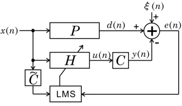
Figure 1 shows a block diagram of the feedforward ANC system considered in this paper. The primary pathPis rep- resented by anNp-tap FIR filter. Its coefficient vector is

p=[p1,p2, . . . ,pN_p]^T, (1)

where^T denotes the transpose of a vector. Each coefficient pi is assumed to be generated from the stochastic process expressed as

hpii=0, D pipi−j

E=κj, (2) and is time-invariant. Here, h·i denotes expectation. If κj = 0 when j , 0 in (2), the elements of the impulse re- sponse of the primary path are uncorrelated with each other.

In this paper, we consider the autocorrelated primary path by introducing the covariance functionκ_j.

The adaptive filterHis anNh-tap FIR filter. Its coeffi- cient vector is

h(n)=[h1(n),h2(n), . . . ,hN_h(n)]^T, (3) wherendenotes the time step. The initial valuehi(0) of each coefficient is assumed to be generated from the stochastic process expressed as

Fig. 1 Block diagram of the feedforward ANC system.

hh_i(0)i=0, D

h_i(0)h_j(0)E

=δ_i,j. (4) Here,δdenotes the Kronecker delta, defined asδi,j=1 (i= j),or 0 (otherwise).Note that the case where hi(0) are all zero can be analyzed in the framework of the present paper by a slight modification of the initial value of the differential equations as described in Sect. 3.

The reference signalx(n) is assumed to be drawn from a distribution with

hx(n)i=0, hx(n)x(n−k)i= rk

Nh

. (5)

The reference signalx(n) is shifted through the tapped-delay line. Therefore, the tap input vectors of the primary pathP and adaptive filterHare

xp(n)=[x(n),x(n−1), . . . ,x(n−Np+1)]^T (6) and

xh(n)=[x(n),x(n−1), . . . ,x(n−Nh+1)]^T, (7) respectively. In the above model, kpk and kh(0)k are O(p

Np)^† and O(√

Nh), respectively. On the other hand, kx_p(n)kandkx_h(n)kareO(1). Here,k·kdenotes the`₂-norm.

The covariance of the reference signal x(n) is normalized byNh in (5). Assuming such a covariance and normalizing the time stepnbyN_h, we can compare the learning curves of different Nh as described later. Note that generality is not lost by this normalization because we can determine the value ofrksuch thatrk/Nhequals the actual covariance. For example, if the actual variance of the reference signal is 0.1 and the actual numberNhof taps of the adaptive filterHis 200, we only have to setr0 = 20. Considering the limit Np,Nh → ∞as described later, we can analytically obtain dynamical behaviors that are independent ofNpandNh. It should also be noted that only the mean and covariance of the distribution are defined in (5). No specific distributions, for example, the Gaussian distribution, are assumed. The same statements are true for both the coefficients of the pri- mary pathPand the initial values of the coefficients of the

†We use the bigOnotation throughout this paper. We express f(N)=O(g(N)) if and only if there exists a positive real numberL and a real numberN0such that|f(N)| ≤L|g(N)|for allN>N0.

adaptive filter H. Ifr_k = 0 whenk , 0 in (5), the refer- ence signal is white. In this paper, we analyze the behavior of the FXLMS algorithm for a nonwhite reference signal by introducing the covariance functionrk.

Since both P andH are FIR filters, their outputs are convolutions of their own coefficients and a sequence of ref- erence signals. That is, the outputsd(n) of the primary path Pandu(n) of the adaptive filterHare

d(n)=p^Txp(n), u(n)=h(n)^Txh(n), (8) respectively.

The secondary pathCis modeled by aK-tap FIR filter.

Its coefficient vector is

c=[c1,c2, . . . ,cK]^T (9)

and is time-invariant. SinceCis also an FIR filter, its output is a convolution of its coefficients and its input sequence.

Therefore, the outputy(n) of the secondary pathCis y(n)=

K

X

k=1

cku(n−k+1). (10)

The error signal e(n) is generated by adding an inde- pendent background noise ξ(n) to the difference between d(n) andy(n). That is,

e(n)=d(n)−y(n)+ξ(n). (11)

Here, the mean and variance ofξ(n) are zero andσ²_ξ, respec- tively.

The LMS algorithm is used to update the adaptive fil- ter. Here, the coefficient vectorcof the secondary pathC is unknown in general. Therefore, the estimated secondary path ˜C, which has been estimated in advance by a certain method, is used to update the adaptive filter. This procedure is called the FXLMS algorithm. When the estimated sec- ondary path ˜Cis aK-tap FIR filter and its coefficient vector is

˜

c=[˜c1,c˜2, . . . ,c˜K]^T, (12) the update procedure obtained by the FXLMS algorithm is

h(n+1)=h(n)+µe(n)

K

X

k=1

˜

ckxh(n−k+1), (13) whereµis the step size.

3. Theory

In this section, we theoretically analyze the behaviors of the FXLMS algorithm using a statistical-mechanical method.

From (10) and (11), the MSE is expressed as follows[34]–

[37].

De²(n)E

=D d²(n)E

+

K

X

k=1 K

X

k⁰=1

ckck⁰u(n−k+1)u(n−k⁰+1)

−2

K

X

k=1

ckhd(n)u(n−k+1)i+σ²_ξ (14) Equation (14) includes many means of the products of uanduand the products ofdandu, including cases where their time steps are different. To calculate these products, we introduce theNh-dimensional vectors

kj(n)=[kj,1(n),kj,2(n), . . . ,kj,N_h(n)]^T. (15) Here, j=−M, . . . ,Mand the elements of the vectors are

kj,i(n)=hmod(i+j−1,N_h)+1(n), (16) where mod(i+j−1,Nh) denotes the remainder wheni+j−1 is divided byNh. Therefore, (15) and (16) indicate that shifts of up toMare considered. This means that the correlations for up to M shifts are considered as described later. Note that k₀(n) = h(n). Here, the fact that k_j(n) is the shifted vector ofh(n) is important. Although (16) expresseskj(n) as the circularly shifted vector of h(n), circular shifting is not essential. In the long-filter assumption described below, generality is not lost even if we assume a linearly shifted vector instead of a circularly shifted vector because the ef- fect of the ends ofh(n) andk_j(n) can be ignored macroscop- ically since these vectors are infinitely long in the long-filter assumption.

In the following, long filters, that is,Np,Nh → ∞, are assumed. This condition corresponds tothe thermodynamic limitin statistical mechanics[25]. With this assumption, we can deterministically describe the macroscopic behaviors of the system, as described later, although the reference sig- nal is stochastically generated. The long-filter assumption is more acceptable than the independence assumption[9]–

[15]used in the literature since the numbers of taps of the unknown system and the adaptive filter are usually large in actual acoustic systems.

If the shift numberjisO(1), we obtain

h(n)^Tx_h(n)=k_j(n)^Tx_h(n−j). (17) Equation (17) is justified in Appendix A. Equation (17) is based on the fact that the shift of the tap input vector is can- celed by the shift of the elements of the adaptive filter. Here, the effect of the ends of the adaptive filter can be ignored since bothh(n) andkj(n) areNh-dimensional, i.e., infinitely long, vectors. Equation (17) implies that the shift j in the time direction can be replaced by the subscript of vectork.

In addition, we consider that a= Np

Nh

(18) is kept constant and introduce two macroscopic variables Rj(n) andQj(n) defined by

R_j(n)= 1

¯ aNh

¯ aNh

X

i=1

p_ik_j,i(n), (19)

Fig. 2 Relationships amongp,h,k, and correlationsRandQ.

Qj(n)= 1 N_h

N_h

X

i=1

hi(n)kj,i(n). (20) Here, ¯ais the smaller value ofaand 1, that is,

¯

a=min(a,1). (21)

Considering (16), it can be seen that Rj(n) and Qj(n) are equal to the means of p_ih_i+j(n) and h_i(n)h_i+j(n), respec- tively. That is, Rj(n) and Qj(n) are the cross-correlation between pandh(n) and the autocorrelation ofh(n), respec- tively. Figure 2 shows the relationships among the vectors and the correlations. Note thatQj(n) is symmetric, that is, Qj(n) = Q−j(n), from the definitions of Qj(n) and kj(n).

Q0(n) is the mean ofh²_i(n) and is omitted in Fig. 2.

Then, we obtain hd(n−j)u(n)i=a¯

M

X

i=−M

Ri(n)ri−j, (22)

hu(n−j)u(n)i=

M

X

i=−M

Qi(n)ri−j, (23)

hd(n−j)d(n)i=a

L

X

i=−L

κiri−j. (24)

Equations (22) and (24) are derived in detail in Appendix B and Appendix C, respectively. As described in Appendix B, we derived (22) based on the assumption that the correlation betweenh(n) andx_h(n) is small[16]–[18]. As described in Sect. 1, theoretical treatment of the LMS algorithm is in- tractable[6]. Therefore, we tackle this difficult problem by using the above small-correlation assumption and the long- filter assumption. Equation (23) is obtained in the same manner as (22). Equations (22) and (23) indicate that the correlations for up to only Mshifts are considered. There- fore, the 2M+1 vectors{kj}, j=−M, . . . ,Mare considered and it is assumed thatRj=Qj=0 when|j|>M. The larger the value of M, the larger the computational cost and the more precisely the theory can predict the simulation results as shown later. In (24),Lis the range in which two elements of the primary path have some correlation. From (22)–(24), we can express the MSE (14) in terms ofR_j(n) andQ_j(n) as

De²(n)E

=

K

X

k=1

c_k

M

X

i=−M K

X

k⁰=1

c_k⁰Q_i(n)ri−k+k⁰

−2¯aRi(n)ri+k−1

! +a

L

X

i=−L

κiri+σ²_ξ. (25) This formula shows that the MSE is a function of the macro- scopic variablesRj(n) andQj(n). Therefore, we derive dif- ferential equations that describe the dynamical behaviors of these variables in the following.

We first derive a differential equation forRj(n). When the coefficient vectorh(n) of the adaptive filter is updated, the j-shifted vectork_j(n) is also changed. This change can be described as

kj(n+1)=kj(n)+µe(n)

K

X

k=1

˜

ckxh(n−k+1−j). (26) Note that the time step of the tap input vectorx_h in (26) is shifted by jcompared with that in (13). We define theNh- dimensional vector ¯pas

¯

p=[p1,p2, . . . ,paN¯ _h,0, . . . ,| {z }0

(1−¯a)Nh

]^T. (27)

Multiplying both sides of (26) on the left by ¯p^T and using (20), we obtain

¯

aNhRj(n+1)=aN¯ hRj(n)+µe(n)

K

X

k=1

˜

ckd(n−k¯ +1−j). (28) Here, ¯d(n)=¯p^Tx_h(n). Then, we obtain

Dd(n¯ −j)u(n)E

=hd(n−j)u(n)i, (29) Dd(n¯ −j)d(n)E

= a¯

ahd(n−j)d(n)i. (30) In (28), the left-hand side and the first term on the right- hand side areO(N_h) and the other term isO(1). This means that the coefficient vectorh(n) of the adaptive filter should be updatedO(Nh) times to changeRj(n) by O(1). There- fore, we introduce timet =n/Nhand use it to represent the adaptive process. Setting the variance and covariance of the reference signal x(n) to be O(N_h⁻¹) as in (5) and consider- ing the limit Nh → ∞, we can deterministically describe the system’s behavior using a small number of macroscopic variables as follows. Then, t becomes a continuous vari- able since the limitN_h → ∞is considered. This is a stan- dard method in the statistical-mechanical analysis of on-line learning[31].

If the adaptive filter is updatedbNhdtctimes in an in- finitely small time dt, we can obtain bNhdtc equations as follows:

¯

aNhRj(n+1)=aN¯ hRj(n) +µe(n)

K

X

k=1

˜

c_kd(n¯ −k+1−j), (31)

¯

aN_hR_j(n+2)=aN¯ _hR_j(n+1) +µe(n+1)

K

X

k=1

˜

c_kd(n¯ −k+2−j), (32)

... ... ...

¯

aNhRj(n+bNhdtc)=aN¯ hRj(n+bNhdtc −1) +µe(n+bNhdtc −1)

×

K

X

k=1

˜

ckd(n¯ −k+bNhdtc − j), (33) where bNhdtc denotes the largest integer not greater than Nhdt. Summing all these equations, we obtain

¯

aNh(Rj+dRj)=aN¯ hRj

+bNhdtcµ

×

* e(m)

K

X

k=1

˜

ckd(m¯ −k+1− j) +

. (34) Here, from the law of large numbers, we have represented the effect of the probabilistic variables by their means since the updates are executedbNhdtctimes, that is, many times, to changeR_jbydR_j. This property is calledself-averaging in statistical mechanics[25]. In (31)–(33), the difference in the time steps of eand ¯d is−k+1− j. To express this, an auxiliary time stepmhas been introduced in (34). From (10), (11), (22), (24), (29), (30), and (34), we obtain a dif- ferential equation that describes the dynamical behavior of Rjin a deterministic form as follows:

dR_j dt =µ

K

X

k⁰=1

˜ ck⁰

L

X

i=−L

κ_iri+k⁰+j−1

−

K

X

k=1

ck M

X

i=−M

Riri+k−k⁰−j

!

. (35)

Next, multiplying (13) by (26) and proceeding in the same manner as for the derivation of the above differential equation forRj, we can derive a differential equation forQj, which is given by (36), where sgn(·) andΘ(·) are the sign function and step function defined by

sgn(x)=1 (x≥0), or −1 (otherwise), (37) Θ(x)=1 (x≥0), or 0 (otherwise), (38) respectively. In addition,

α= Θ(γ)γ−k⁰⁰, β= Θ()−k⁰⁰, (39)

γ= j+1−k⁰, =−j+1−k⁰. (40)

Here, we have to treat the correlations carefully and execute complicated calculations since the past tap input vectors x_h affect both the coefficient vectorhof the adaptive filter and its shifted vector k_j. The derivation of (36) is outlined in Appendix D.

Equations (35) and (36) are first-order ordinary differ- ential equations with 3M+2 variables since the correlations for up to Mshifts are considered as described before. That is,

d

dtz=Gz+b, (41)

dQj

dt =µ

K

X

k⁰=1

˜ ck⁰

( M

X

i=−M

"

¯ aRi

ri−γ+ri−

−

K

X

k=1

ckQi

ri−k⁰+k+j+ri−k⁰+k−j

#

−µ

"

sgn(γ)

|γ|

X

k⁰⁰=1

δ_α,0σ²_ξ+a

L

X

i=−L

κ_ir_i+α

−

K

X

k=1

ck M

X

i=−M

¯

aRiri+k−1−α+aR¯ iri+k−1+α−

K

X

k⁰⁰⁰=1

ck⁰⁰⁰Qiri−k+k⁰⁰⁰−α

! ^K X

i=1

˜

cirk⁰−i−j+α

+sgn()

||

X

k⁰⁰=1

δβ,0σ²_ξ+a

L

X

i=−L

κiri+β

−

K

X

k=1

ck M

X

i=−M

¯

aRiri+k−1−β+aR¯ iri+k−1+β−

K

X

k⁰⁰⁰=1

ck⁰⁰⁰Qiri−k+k⁰⁰⁰−β

! K

X

i=1

˜ cirk⁰−i+j+β

#)

+µ²

" K

X

k=1

c_k

M

X

i=−M K

X

k⁰=1

c_k⁰Q_iri−k+k⁰−2¯aR_ir_i+k−1

! +a

L

X

i=−L

κ_ir_i+σ²_ξ

# K

X

k⁰⁰=1 K

X

k⁰⁰⁰=1

˜

c_k⁰⁰c˜_k⁰⁰⁰r_k⁰⁰−k⁰⁰⁰−j, (36)

z=[Q₀, . . . ,Q_M,R−M, . . . ,R₀, . . . ,R_M]^T. (42) Here, the matrixGand vectorbare determined by (35) and (36). For example, the (2M+2+j,2M+2+i) element of the matrixGis equal to the coefficient ofRi on the right-hand side of (35), that is,

G_ji=−µ

K

X

k⁰=1

˜ c_k⁰

K

X

k=1

c_kr_i+k−k⁰−j, (43) where−M≤i,j≤M. Note thatR0is the (2M+2)th element ofzas shown in (42). As another example, the (2M+2+j)th element of the vectorbis

bj=µ

K

X

k⁰=1

˜ ck⁰

L

X

i=−L

κiri+k⁰+j−1 (44)

as seen on the right-hand side of (35), where−M≤ j≤M.

All initial values ofQj(j,0) andRjare equal to zero becauseh_i(0) and p_iare independently generated. The ini- tial value ofQ0 is unity since the initial valuehi(0) of each coefficient is generated from the stochastic process given by (4). Therefore,zatt=0 is

z(0)=[1,0, . . . ,| {z }0

3M+1

]^T. (45)

Using (45) as the initial condition, we can analytically solve (41) to obtain

z(t)=e^Gt

z(0)−G⁻¹e^−Gtb+G⁻¹b

, (46)

wheree^Dis the matrix exponential function defined by e^D=

∞

X

k=0

1

k!D^k=I+ 1 1!D+ 1

2!D²+· · ·. (47) If we consider the case where the initial values of the

coefficientsh_i(0) are all zero, we can obtain the solution by modifying (45) to

z(0)=[0, . . . ,| {z }0

3M+2

]^T (48)

since the initial value ofQ₀is zero in this case.

The averaging method and the ordinary differential equation (ODE) method are well-known methods for an- alyzing the dynamical behaviors of discrete-time update systems [7], [21], [38], [39]. Here, we describe the dif- ference between these methods and our proposed method.

When the averaging method and ODE method are ap- plied, continuous-time differential equations are derived from discrete-time equations based on the theorem that the dynamical behaviors of the variables correspond to the av- erage behaviors in the small-step-size limit. Therefore, the small-step-size limit is essential in the averaging method and ODE method. In contrast, in our proposed method, the small-step-size condition is not explicitly used. In this case, continuous-time differential equations are derived through the reasonable processes described in this section. Here, we note the following. Although the variance and covariance of the reference signal are normalized byNh, as shown in (5), this normalization is not equivalent to the small-step-size as- sumption. This is because the magnitude of the output of the adaptive filter is kept to the same order whenNhapproaches infinity since not only the variance and covariance of the reference signal become small as shown in (5) but also the length of the adaptive filter becomes large. Therefore, the theory derived in this section is also expected to predict the experimental behaviors of a system in which neither the step size nor the covariance of the reference signal is infinitely small. To show the validity of the theory, in Sect. 4 we com- pare and discuss the results obtained using the theory and simulation results for a primary path and an adaptive filter with finite numbers of taps when neither the step size nor

the covariance of the reference signal is infinitely small.

4. Results and Discussion

In this section, we discuss the validity of the theory obtained in the previous section by comparison with simulation re- sults. The conditions of the analysis and the simulation in the following subsections may not appear to be consistent.

This is because each set of conditions is specifically selected depending on the purpose of each subsection. The main con- ditions in each subsection are summarized in Table 1.

4.1 Learning Curves and Ranges of Correlations

We first investigate the validity of the theory by compar- ison with simulation results regarding the dynamical be- haviors of the MSE, that is, the learning curves. Figure 3 shows the learning curves obtained using the theory in the previous section, along with the corresponding simulation results. The conditions are shown in Table 1. The step size is µ = 0.1. The parameters that determine the vari- ance and covariance of the elements of the primary path are κk = δk,0, that is, the elements of the primary path are un- correlated. The parameters that determine the variance and covariance of the reference signal arerk =δk,0, that is, the reference signal is white. There is no background noise, that is,σ²_ξ=0. In Fig. 3, the curves represent theoretical results and the polygonal lines represent simulation results. In the theoretical calculation, the results are obtained by substitut- ingRjandQj, which are obtained by solving (41), into (25) in the cases where the ranges of the correlations considered areM =0,1,2,6,and 10. Here, (41) is numerically solved by the Runge-Kutta method because the calculation of the analytical solution (46) involves numerical instability^††. In the computer simulations, four given primary paths are used in the both cases of the numbers of taps of the primary path and the adaptive filter are N_p = N_h = 80 and 2000. For all the computer simulations, ensemble means for 200 tri- als are plotted for each given primary path. Each coefficient piof all the primary paths is independently generated from the Gaussian distribution with a mean of zero and variance of unity. Here, note that all of the simulation results using Np =Nh =80 and 2000 and the theoretical results derived usingNp,Nh → ∞can be compared along a single vertical axis because the variance of the reference is normalized by Nh, as shown in (5), and the variablet=n/Nhis introduced instead of the number of updatesn itself as described be- fore. The steady-state MSE, as well as the learning curves, is independent ofNhsince the variance of the reference sig- nal is normalized byN_hin the model assumed in this paper.

All initial values of the coefficientshi(0) are set to zero in the simulation, and the initial condition (48) is used in the

††The numerical instability regarding the analytical solution originates from the fact that the analytical solution includes the ma- trix exponential function defined by (47). Since (47) is expressed as an infinite series, some numerical computations are necessary and instability exists.

Fig. 3 Learning curves obtained theoretically and by simulation. The theoretical results forM=6 andM=10 almost overlap.

theoretical calculation to compare the derived theory with the previous theory in[19]. The reason why the theory in [19]was chosen for comparison is that it is a relatively new theory that avoids the independence assumption and is used to analyze the dynamical behaviors of the MSE, similarly to the theory derived in this paper.

Figure 3 shows that the learning curves obtained by the computer simulations considerably vary in the case ofNp = Nh =80, whereas the variation is small in the case ofNp = N_h = 2000. The theory derived in this paper predicts the simulation results well in the average sense. The larger the value of M, the more closely the theoretical results agree with the average simulation results. The theoretical results for M = 6 andM =10 almost overlap and agree with the average simulation results reasonably well. The long-time dynamical behaviors can be predicted by using a large value ofM.

The four learning curves obtained from the theory in [19], which assumes a small step size and statistical inde- pendence between the adaptive filter and the tap input vec- tors, are shown with thin lines in Fig. 3. In each of the four cases, exactly the same primary path as that used in the com- puter simulations forN_p =N_h=80 has been used. Note that the theory in[19]does not provide an asymptotic analysis.

Therefore, the results depend on the realized concrete val- ues of the primary path. The theoretical results obtained by the theory in [19]excessively vary and are too sensitive to the given primary path. The theory cannot predict the corre- sponding simulation results in the model setting described in this paper. On the other hand, the theory derived in this pa- per predicts the average simulation results reasonably well.

The theory derived in this paper can also predict sim- ulation results for largeNpandNh, i.e., 2000, using a rela- tively smallM, that is, using a small number of macroscopic variables, which is a noteworthy characteristic of the derived theory. It is the fundamental principle of statistical mechan- ics that the behavior of a system composed of a very large number of elements can be represented by a small number of macroscopic variables. Therefore, the expression ‘large Nh’, which is not quantified and appears imprecise, is not inappropriate. Note that Fig. 3 shows that the derived theory can predict average simulation results not only for largeNp

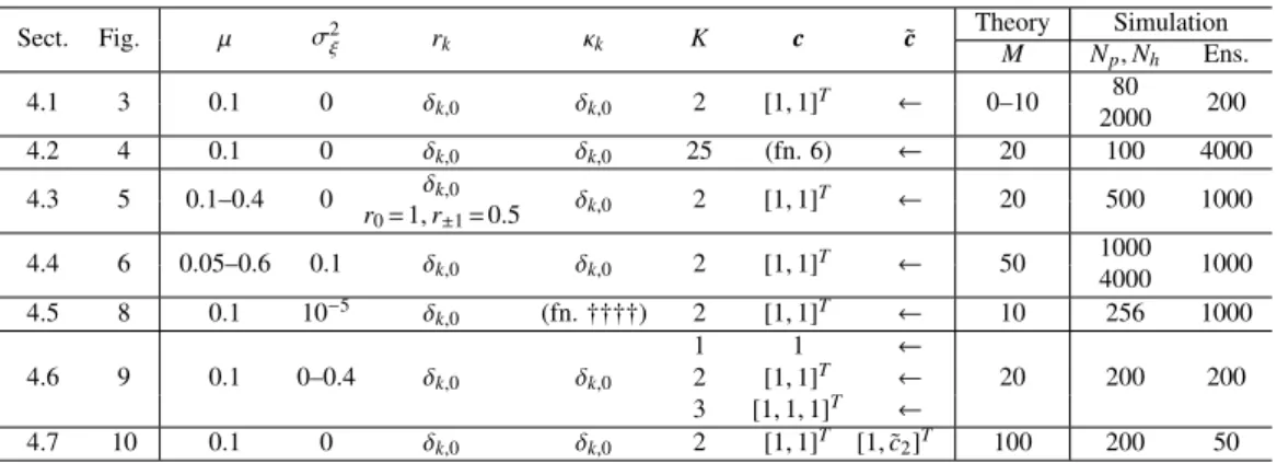
Table 1 Summary of the main conditions.

Sect. Fig. µ σ²_ξ r_k κk K c ˜c Theory Simulation

M N_p,N_h Ens.

4.1 3 0.1 0 δk,0 δk,0 2 [1,1]^T ← 0–10 80

2000 200

4.2 4 0.1 0 δk,0 δk,0 25 (fn. 6) ← 20 100 4000

4.3 5 0.1–0.4 0 δk,0 δk,0 2 [1,1]^T ← 20 500 1000

r0=1,r±1=0.5

4.4 6 0.05–0.6 0.1 δk,0 δk,0 2 [1,1]^T ← 50 1000

4000 1000 4.5 8 0.1 10⁻⁵ δk,0 (fn.††††) 2 [1,1]^T ← 10 256 1000

4.6 9 0.1 0–0.4 δk,0 δk,0

1 1 ←

20 200 200

2 [1,1]^T ←

3 [1,1,1]^T ←

4.7 10 0.1 0 δk,0 δk,0 2 [1,1]^T [1,c˜₂]^T 100 200 50

µ: step size,

σ²_ξ: variance of the background noise,

rk: parameter that decides the autocorrelation of the reference signal, κk: covariance of the elements of the primary path,

K: number of taps of the secondary pathC, c: coefficients of the secondary pathC,

˜

c: coefficients of the estimated secondary path ˜C,

M: range in which the macroscopic variablesR_jandQ_jare considered in the proposed theory, N_p: number of taps of the primary pathPin the simulation,

N_h: number of taps of the adaptive filterHin the simulation,

Ens.: number of trials for which the ensemble means are calculated in the simulation, fn.: footnote,

δ: Kronecker delta.

˜

c₂is varied from−1 to+3 in Sect. 4.7.

andNh, i.e., 2000, but also for relatively small Np andNh, i.e., 80.

There is some background (BG) noise in actual situa- tions where ANC is applied. Previous studies[12]and[19]

also treated the case where there is some BG noise. How- ever, when there is BG noise, the accuracy of the theory is unclear since the MSE is buried in the BG noise. In contrast, much higher accuracy is needed when attempting to use the theory to predict the simulation results in the case of no BG noise. Therefore, to verify the theory, it is more rigorous and reasonable to show the agreement with simulation re- sults in the case of no BG noise. For this reason, the results for a case with no BG noise are shown in Fig. 3. Of course, the proposed theory is also valid when there is BG noise, as shown later in Figs. 6, 8, and 9.

4.2 Long Impulse Response of Secondary Path

Figure 3 shows the results forK =2, that is, the secondary path has a small number of taps. Next, we investigate the case of a largeK to show the effectiveness of the obtained theory in a more realistic case. Figure 4 shows the result for K=25. In both the theoretical calculation and the computer simulations, the coefficient vectorcof the secondary path is the normalized version of the vector reported in[2]^†††. The

†††c = [−0.073844, 0.280609, −0.778907, −0.321869, 2.563927, −5.876712, 11.504314, −18.114344, 25.967108,

−33.871861, 41.345085, −47.070049, 50.785450, −51.863720, 50.043129, −45.990845, 39.786583, −33.078777, 25.692730,

−18.861567, 12.781915, −8.174841, 4.567914, −2.076808, 0.728670]^T

Fig. 4 Learning curves obtained theoretically and by simulation when K=25.

initial coefficients h_i(0) are independently generated from the Gaussian distribution with a mean of zero and variance of unity in the simulation, and the initial condition (45) is used in the theoretical calculation. Ensemble means in the simulation are taken by averaging over not only the refer- ence signals but also the stochastically generated primary path. The other conditions are shown in Table 1. Figure 4 shows that the theory also predicts the average simulation results when the number of taps of the secondary pathKis large.

4.3 Nonwhite Reference Signal

Figures 3 and 4 show the results for white reference sig- nals. However, the reference signal is not necessarily white in the actual application of an ANC system. Therefore, we next investigate the case of a nonwhite reference signal

Fig. 5 Learning curves obtained theoretically and by simulation when the reference signal is white and nonwhite.

to show the effectiveness of the obtained theory. Figure 5 shows the learning curves obtained theoretically along with the corresponding simulation results[36]. The correlation functions of the reference signal arer_k = δ_k,0 (white) and r0 =1,r±1 =0.5,r±k=0 whenk≥2 (nonwhite). The ini- tial coefficientsh_i(0) are independently generated from the Gaussian distribution with a mean of zero and variance of unity in the simulation, and the initial condition (45) is used in the theoretical calculation. Ensemble means in the sim- ulation are taken by averaging over not only the reference signals but also the stochastically generated primary path.

The other conditions are shown in Table 1.

Figure 5 shows that the theoretical results agree with the simulation results including the difference between the behaviors for white and nonwhite reference signals. It is also shown that the upper bound of the step sizeµfor the white reference signal is larger than 0.4, whereas that for the nonwhite reference signal is smaller than 0.4 because the learning curve ofµ = 0.4 for the nonwhite reference signal diverges.

4.4 Effect of Step Size on Learning Curves

We next investigate the relationship between the step sizeµ and the learning curves. This is important from the view- point of the actual application of ANC systems.

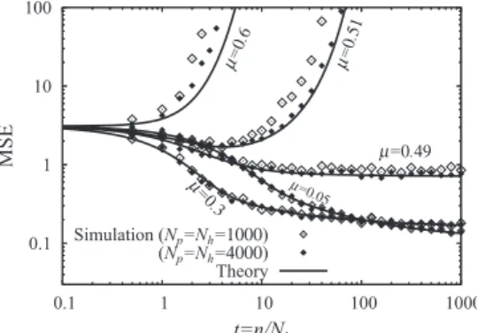
Figure 6 shows the learning curves obtained theoret- ically along with the corresponding simulation results for various step sizesµ. The variance of the background noise isσ²_ξ =0.1. The initial coefficientshi(0) are independently generated from the Gaussian distribution with a mean of zero and variance of unity in the simulation, and the initial condition (45) is used in the theoretical calculation. Ensem- ble means in the simulation are taken by averaging over not only the reference signals but also the stochastically gener- ated primary path. The other conditions are shown in Ta- ble 1.

Figure 6 shows that the theoretical results agree with the simulation results reasonably well when µ is smaller than 0.5. However, there is significant disagreement when µ ≥ 0.5. The simulation results for Np = Nh = 4000 more closely agree with the theoretical results than those for

Fig. 6 Learning curves for various step sizesµobtained theoretically and by simulation.

Fig. 7 Example of impulse response of an actual primary path.

Np =Nh =1000. The reason for this disagreement is con- sidered to be that the theory is derived using the long-filter assumption, that is, Np,Nh → ∞, whereas the simulations are executed using finite values ofN_p andN_h. The depen- dence of the bias on the system size is an example of the phenomenon known asthe finite-size effectin statistical me- chanics. The condition ofµ=0.5 corresponds to the phase transition point at which the MSE changes from being con- vergent to divergent. Figure 6 shows that this theory quanti- tatively predicts the simulation results for a finite number of taps when the step size is smaller than the transition point, which is usually the case for the FXLMS algorithm.

4.5 Actual Primary Path

In the derivation of the theory, the elements piare assumed to be stochastically generated as shown in (2). In addi- tion, Fig. 3 shows the results forκk =δk,0, that is, the case where the elements of the primary path Pare uncorrelated.

However, the actual elements of the impulse response of a primary path are not stochastic but deterministic. In ad- dition, the elements are generally strongly correlated with each other, that is, the primary path has a strong autocorre- lation. For example, Fig. 7 shows an example of the impulse response of a primary path obtained experimentally[37]^††††. While the variance of the elements of the impulse response

††††The autocorrelations of this primary path are ˆκj ≡

1 N_P−j

PN_P

i=1+jpipi−j are (1.211, 0.963, 0.392, −0.134, −0.363,

Fig. 8 Learning curves obtained theoretically and by simulation in the case of the actual primary path.

of this primary path is ˆκ₀ ≡ ¹

NP

PNP

i=1p²_i = 1.211×10⁻³, the correlation between the neighboring elements is ˆκ1 ≡

1 NP−1

PNP

i=2pipi−1 = 0.963×10⁻³. This indicates that there are strong correlations between the elements of the impulse response of the actual primary path. Therefore, it is im- portant to investigate whether the derived theory can predict the behaviors of computer simulations using the impulse re- sponse of the actual primary path. For this purpose, the the- ory can absorb the characteristics of the primary path by settingκ_j=κˆ_j, whereκ_jis defined by (2).

Figure 8 shows the learning curves obtained theoreti- cally along with the corresponding simulation results in the case of the actual primary path[37].

In the theoretical calculations, the results of six cases are plotted, that is, jmax=0,1,2,5,10,and 20. Here,jmax is the maximum value of the subscriptjofκ_jdefined by (2).

For example, jmax = 0 means that κj = 0,|j| > 0, that is, the theory only considers the variance of the elements of the impulse response of the primary path. jmax = 2 means that κ_j = 0,|j| > 2, that is, the theory consid- ers κj,j = −2,−1,0,1,2. In the computer simulations, Nh = Np = 256 and ensemble means for 1000 trials are plotted. The impulse response of the primary path in the computer simulation is that shown in Fig. 7, that is, the ac- tual impulse response measured experimentally. Note that the ensemble means are obtained by averaging over only ref- erence signals. This averaging is different from that in the simulations in Sects. 4.1–4.4, where the ensemble means are obtained by averaging over both reference signals and chan- nels. The other conditions are shown in Table 1.

Figure 8 shows that the theory forjmax=0, that is, the theory only using the variance, cannot predict the behaviors of the computer simulation. The theory for jmax =1 also cannot predict the behaviors. However, the larger the value of jmax, the more closely the theoretical results agree with the simulation results. The theoretical results forjmax=10

−0.312, −0.161, −4.41, 0.0156, 0.0406, 0.0284, −0.0243,

−0.0757, −0.0680, −0.00586, 0.0290,−0.0362,−0.177,−0.287,

−0.286,−0.184)×10⁻³.

Fig. 9 Relationship between step sizeµand steady-state MSE obtained theoretically and by simulation.

and 20 almost overlap and agree with the simulation results reasonably well.

As described in this section, by using the autocorrela- tions of the primary path, the derived theory can predict the behaviors in the case of an actual primary path. This shows that even if the realized values of the actual elements, which are inherently deterministic, of the impulse response of the primary path are not known, the theory can predict the be- haviors in the case of an actual primary path through the statistic ˆκ.

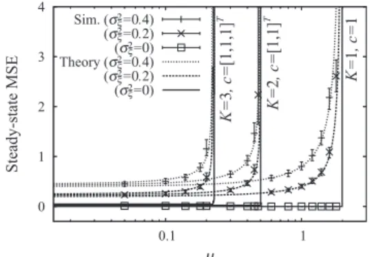
4.6 Steady-State MSE

We next investigate the steady-state MSE on the basis of the derived theory. Steady-state values ofRandQcan be cal- culated by letting the left-hand side of (41) be a zero vector.

That is, the steady-state valuez_stofzis

zst=−G⁻¹b. (49)

Substituting the obtained steady-stateRandQ, that is, the elements of z_st, into (25), we analytically obtain the steady- state MSE. We compare the theoretically obtained steady- state MSE and simulation results. The conditions regarding the numberKof taps and the coefficient vectorcof the sec- ondary pathC are K = 1 (c = 1), K = 2 (c = [1,1]^T), and K = 3 (c = [1,1,1]^T). The variances of the back- ground noise are σ²_ξ =0,0.2, and 0.4. Figure 9 shows the results obtained theoretically and by simulation[35]. In the computer simulations, the medians and standard deviations of the 200 squared errors fromt = 9000 tot = 11000 in 200 trials are plotted using error bars. These values oftin the simulations are sufficient for the MSE to reach a steady- state value. Ensemble means in the simulation are taken by averaging over not only the reference signals but also the stochastically generated primary path. The other conditions are shown in Table 1. The theoretical results agree with the simulation results reasonably well in Fig. 9.

4.7 Effect of Estimation Error of Secondary Path

Figures 3–9 show results in the case of ˜c= c, i.e., the esti- mated secondary path has no error. However, the estimated

Fig. 10 Relationship between estimated secondary path and steady-state MSE.

secondary path inevitably has some error in actual active noise control. Therefore, it is important to investigate its effect. The obtained theory is also applicable to cases where the secondary path estimation has some error since the the- ory treats the secondary path and the estimated secondary path separately.

Figure 10 shows the relationship between the estimated secondary path and the steady-state MSE obtained theoret- ically along with the corresponding simulation results. The secondary pathCis a two-tap FIR filter, that is,K=2, and its coefficients arec1 = c2 = 1. The first element of the estimated secondary path is ˜c₁ =1 and the second element is varied from ˜c2 = −1 to+3. The step size is µ = 0.1.

In the computer simulations, the means and standard devi- ations of 50 squared errors in the case of t = 10000 are plotted using error bars. In the theoretical calculation, the steady-state MSE is obtained by the calculation described in Sect. 4.6. Ensemble means in the simulation are taken by averaging over not only the reference signals but also the stochastically generated primary path. The other conditions are shown in Table 1.

When ˜c2 = 1, which corresponds to no estimation er- ror, the steady-state MSE is minimized. The larger the es- timation error, the larger the steady-state MSE. The theo- retical results qualitatively agree with the tendency of the simulation results in Fig. 10.

The so-called 90^◦ condition [40]–[42]is well known for stability of the feedforward ANC. According to the 90^◦ condition, the phase error between the secondary pathCand the estimated secondary path ˜C has to be in the region of

−π/2 to π/2 for the MSE to converge. This condition is equivalent to that the argument ofC(ω)/C(ω) has to exist˜ in the region of−π/2 toπ/2. Here,ωdenotes the angular frequency. C(ω) and ˜C(ω) denote the frequency responses ofCand ˜C, respectively.

WhenK=2, we obtain C(ω)

C(ω)˜ = c1+c2e^−jω

c˜1+c˜2e^−jω. (50) We can easily calculate the real part of (50) as

c1c˜1+c2c˜2+(c1c˜2+c˜1c2) cosω

((˜c₁+c˜₂) cosω)²+(˜c₂sinω)² . (51)

Here, the denominator of (51) is obviously positive. There- fore, the numerator of (51) should be positive for the argu- ment of C(ω)/C(ω) to exist in the region of˜ −π/2 toπ/2.

That is, the necessary condition for stability is

c1c˜1+c2c˜2+(c1c˜2+c˜1c2) cosω >0. (52) Substitutingc1=c2=c˜1 =1, that is, the conditions in this subsection, into (52), we obtain

(1+c˜₂)(1+cosω)>0. (53) Therefore, the condition for stability is

˜

c₂>−1. (54)

It can be seen that the behavior in Fig. 10 is consistent with (54).

However, the 90^◦ condition is valid for the infinitely small step sizeµ[41],[42]. This means that the 90^◦con- dition is not a sufficient condition but a necessary condition when the step sizeµis not infinitely small. Therefore, the right-hand side of (54) does not agree with the value of ˜c2

for which the MSE diverges in Fig. 10.

The necessary and sufficient condition in the case where the step size is not infinitely small was derived in [41],[42], written by one of the authors of this paper. The condition is

1−µkx_h(n)k²C(ω) ˜C^∗(ω)

<1, (55) where∗denotes the complex conjugate.

Substitutingµ=0.1,kxh(n)k=1, andc1 =c2 =c˜1 = 1, that is, the conditions in this subsection, into (55) and nu- merically calculating the lower bound of ˜c2satisfying (55) for arbitrary ω in the region of−π < ω < π, we obtain

−0.7802 as the lower bound of ˜c2. This bound is exactly in agreement with the behavior in Fig. 10. This indicates that the theory derived in this paper and the theory derived in[41], [42]justify each other. The authors consider this justification to be significant.

5. Conclusions

We have analyzed the behaviors of active noise control with the FXLMS algorithm using a statistical-mechanical method. The obtained theory can treat not only a white ref- erence signal but also a nonwhite reference signal. In ad- dition, we have also shown that the theory can predict the behaviors in the case of an actual primary path by using the autocorrelations of the actual primary path. Furthermore, the effect of the estimation error of the secondary path was investigated using the derived theory. The theory quantita- tively agrees with the results of computer simulations. The principal assumption used in this paper is that the tapped- delay lines of the primary path and the adaptive filter are sufficiently long.