Dynamics of water circulation and anthropogenic activities in paddy dominant watersheds

(1)

Dynamics of water circulation and anthropogenic activities in paddy dominant watersheds

−− From field-scale processes to catchment-scale models −−

Takeo Yoshida

Hydrology and Water Resources Management, Hydraulic Engineering Research Division

Abstract

Irrigation in Japan accounts for 70% of total water diversion and is predominantly used for rice cultivation. Water movement within irrigated areas is complicated not only by the substantial volumes involved but also by repeated cycles of diversion and return flow, by which diverted water gradually drains from irrigated areas. Thus, understanding tivater use and its management is crucial for characterizing flow regimes in watersheds where irrigated paddies predominate. Recent changes in our natural and social environments are increasing the vulnerability of the water resources used for rice irrigation, which has been designed and operated under the assumption of stationarity. Distributed hydrological models have often been used to assess the vulnerability of water resources. However, although the importance of such assessments in analyzing anthropogenic water use in catchment-scale hydrological systems is being increasingly recognized, few models have attempted to incorporate the dynamics of water circulation associated with rice paddy irrigation. A model suitable for assessing water resources for rice irrigation must have the following capabilities. First, it must simulate water movements within irrigated rice fields, including water diversion from rivers, allocation through channels, and return flow from irrigated areas. Second, it should represent natural hydrological cycles in the whole watershed and should, integrate natural and anthropogenic water movement within the watershed.

In this thesis, the author presents an integrated model that couples catchment-scale natural hydrological cycles and human- related water cycles in irrigated paddy areas; hereafter the catchment-scale water circulation model. The main objective of model development is to assess the interaction between human-related and natural water cycles, especially in watersheds where densely irrigated paddies are dominant. Chapter 2 introduces the base model for this study. The base model simulates the interaction between catchment-scale hydrological cycles and paddy water uses. The author also traces some of the shortcomings of the base model and outlines the concept of the new model. In Chapter 3 presents the core issue of this thesis to be addressed: the representation of water circulation in densely developed irrigated paddy areas, and the integration of this model with natural hydrological cycles. The newly developed model is applied to a typical watershed in which irrigated paddies are dominant in Japan, and the interaction between natural and anthropogenic water cycles are evaluated. In Chapters 4 and 5, for extend the applicability of the new model, sub-models for snowmelt and flood inundation processes are introduced and validated. Finally, in Chapter 6, the catchment-scale water circulation model is applied to three experimental watersheds, each of which is donunated by different land uses and cultivation statures: namely cultivated paddies, abandoned paddies, and forest. We then discuss the ability of the new model to reproduce the hydrological changes associated with physical changes in paddy conditions.

The concepts in the model should contribute to ongoing discussions on how to incorporate anthropogenic impacts into distributed hydrological models. There are two potential beneficiaries of this model: the climate-change impact-assessment community and managers of water resources in paddy-dominant watersheds. A number of studies have examined the impacts of climate change on water resources. However, the effects of anthropogenic water cycles in paddy-dominant watersheds have not yet been examined explicitly, and thus the impact of climate change on paddy water-use systems is not fully understood. The proposed model calculates both natural and anthropogenic water cycles in watersheds. It thus provides not only stream flow changes, but also the potential effects of climate change on reservoir storages and the amounts of water diverted for paddy irrigation. Also, the model has the potential to contribute to water resources management, especially in watersheds undergoing rapid societal change.

The expected societal changes in paddy-dominant watersheds in Japan will lead not only to an increase in the number of abandoned paddies, but also to increases in the number of crop varieties used and the length of irrigation periods, or increases in water demand due to changes in field water management. Moreover, in developing countries in the Asian Monsoon region, the area under irrigation and the number of reservoirs being developed are increasing at a tremendous rate. This model should be highly useful in the planning for optimum management of such watersheds.

Keywords:catchment, distributed hydrological model, rice paddies, irrigation, water resources 農工研報54

!# "

$ 1〜72, 2015

(2)

CONTENTS

1. Introduction ………3

1.1 Background ………3

1.2 Previous research on modeling watersheds with rice paddy irrigation ………4

1.2.1 Distributed hydrological models and their application in water resources assessment ………4

1.2.2 Catchment-scale interactions between rice paddy irrigation and hydrological cycles ………4

1.2.3 Status of paddy cultivation and runoff characteristics ………5

1.3 Objective and methods ………5

1.4 Thesis outline ……….6

2. Structure of the base model and novel concepts in the newly developed model ………6

2.1 Introduction ………6

2.2 Basic structure of the base model ……… 6

2.2.1 Runoff module ………6

2.2.2 Cropping pattern and area module ………8

2.2.3 Actual ET module ………8

2.2.4 Paddy water use module ………8

2.3 Novel concepts introduced in the new model 8 2.4 Summary ……… 9

Appendix 2: Calculation of Reference Evapotranspiration ………9

3. Modeling of water circulation in river basins pos- sessing large areas of irrigated paddy by incorpo- ration of a water allocation and management mod- ule ………9

3.2 Structure of water allocation and management module ………10

3.2.1 Reservoir operation scheme ………10

3.2.2 Water allocation scheme ………11

3.3 Study watershed ………12

3.3.1 Topography, geology and climate of the study watershed ………12

3.3.2 Agricultural water use in the basin ……12

3.3.3 Collected data and data input procedures ………12

3.3.4 Settin s for the water allocatto and management module ………14

3.4 Results aild discussion ………14

3.4.1 Validation of model with rivere discharges ………14

3.4.2 Changes to the flow regime simulated by the reservoir operation scheme …………15

3.4.3 Estimated water circulation within an irrigated areas ………15

3.4.4 Retei-n 1-atio of divet-ted water from irrigated areas ………16

3.5 Summary ………17

Appendix 3 ………19

Appendix 3A: Hydrographs at Takada ………19

Appendix 3B: Changes in calculated discharges at Futagojima due to incorporation of water allocation and management module …20 Appendix 3C: Changes in calculated discharges at Takada due to incorporation of return flow processes into the model …………21

4. A snowfall and snowmelt module for warm climate watersheds and its integration into DWCM-AgWU ………22

4.1 Introduction ……… 22

4.2 Development of the snowfall and snowmelt module ………22

4.2.1 Estimation of snowmelt based on the en- ergy balance ………22

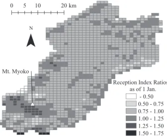
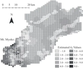
4.2.2 Estimation of the spatial extent of parameter ksl ………23

4.3 Study watershed ………24

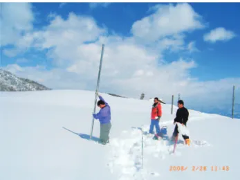
4.3.1 Winter- precipitation in the study watershed ………24

4.3.2 Collected winter precipitation data ……24

4.4 Results and discussion ………25

4.4.1 Estimated spatial distribution of parameter ksl ………25

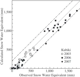
4.4.2 Comparison of observed and calculated SWE ……… 26

4.4.3 Calculated river discharges after incorporation of the developed snowfall and snowmelt module ……… 27

Appendix 4A: Time series of SWE at all the observed points included in the Kubiki Area ………29

Appendix 4B: Time series of SWE at all the observed points included in the Ikenodaira Area ………32

Appendix 4C: Time series of SWE at all the ob-served points included in the Ｍyoko Area ………33

Appendix 4D: Time series of SWE at all the observed points included in the Iiyama Area ………34

Appendix 4E: Hydrographs in winter (from De- cember through May) ………35

5. Integration of an inundation module for low- gradient rivers into DWCM-AgWU ………36

5.2 Representation of inundation processes and its integration into DWCM-AgWU ………36

(3)

5.2.1 Development of inundation module for low-gradient 1-ivers ………36 5.2.2 Integration of the inundation module into

DWCM-AgWU ………36

5.3 Study watershed ………37 5.3.1 Inundation in the study watershed ……37 5.3.2 Data collection in the study watershed 37 5.4 Results and discussion ………39

5.4.1 Application to the case study

watershed ……… 39

5.4.2 River flows without the inundation

module ………39

5.4.3 River flows with the inundation

module ……… 39

Appendix 5A: Observed discharges and calculated discharges with/without inundation processes at the Mahaxay flow gauge …41 Appendix 5B: Observed and calculated dis-

charges with/without inundation processes at the Xebanfai Bridge flow gauge …… 42 6. Short-term runoff modelling in hilly watersheds

where paddy fields are prevalent ………43

6.2 Experimental watersheds and hydrological

observation ………43

6.2.1 Study area ………43 6.2.2 Selection of experimental watersheds …43 6.2.3 Hydrological observations and data anal-

ysis ………44 6.3 Comparison of runoff characteristics based on

paddy cultivation conditions ………46 6.3.1 Comparison of runoff ratios ………46 6.3.2 Comparison of peak runoff coefficients 46 6.3.3 Comparison of retention characteristics 47 6.3.4 Changes in peak runoff coefficients and

runoff with more abandoned paddies …48 6.4 Rainfall-runoff modelling of watersheds charac-

terized by terraced paddy ………48 6.4.1 Modelling runoff processes in cultivated

and abandoned paddies ………48 6.4.2 Initial conditions for short-term calcula-

tions ………49

6.4.3 Model application to experimental water-

sheds ………49

6.5 Results ………50

6.5.1 Comparison of discharges and storage in unsaturated and saturated zones calculated at different time intervals ……… 50 6.5.2 Results of short-term runoff calculations

and comparison with observed values …51 6.5.3 Initial conditions for short-term calcula-

tions ………53

6.5.4 Effects of initial soil wetness on short- term runoff characteristics . ………53

Appendix 6: Observed discharges and calculated discharges in the rainfall events listed in Table 5 56

7. Conclusion ……… 65

7.1 Main findings ………65

7.2 Outlook ………66

1. Introduction 1.1 Background

Irrigation in Japan accounts for 70% of the total water diversion and is used predominantly for rice cultivation. Water movement within irrigated areas is complicated not only by the substantial volumes involved but also by repeated cycles of diversion and return flow, when diverted water gradually drains from the irrigated areas. Understanding the dynamics of return flow is crucial for characterizing flow regimes in watersheds where irrigated paddies predominate.

Recent changes in our natural and social environments are in creasing the vulnerability of the water resources used for rice irrigation, which uses systems that were designed and are operated under the assumption of stationarity (Milly et al., 2007). Distributed hydrological models are often used to assess the vulnerability of water resources. However, although the importance of such assessments in analyzing anthropogenic water use in catchment-scale hydrological systems is being increasingly recognized, few models have attempted to incorporate the dynamics of water circulation associated with rice paddy irrigation.

A model suitable for assessing water resources for rice irrigation must have the following capabilities. First, it must simulate water movements within irrigated rice fields, including water diversion from rivers, its allocation through channels, and the return flow from irrigated areas. Second, it should also represent natural hydrological cycles in the whole watershed and should integrate natural and anthropogenic water movements within the watershed.

In this thesis, I presents an integrated model that couples catchment-scale natural hydrological cycles with human-related water cycles in irrigated paddy areas. The main objective was to produce a model that could be used to assess the interaction between the human-related and natural water cycles, especially in watersheds where densely irrigated paddies are dominant. In addition, to extend the applicability of the model to a broad range of hydrological conditions, several sub-models were developed for representing flooding and snow-melting

(4)

processes and subsequently integrated into the catchment-scale water circulation model.

1.2 Previous research on modeling watersheds with rice paddy irrigation

1.2.1 Distributed hydrological models and their application in water resources assessment Hydrological models are categorized into lumped models and distributed models according to how they spatially represent hydrological processes. Lumped models are developed to predict stream flow at a point of in- terest in a watershed based on the storage-discharge re- lationships. In contrast, Freeze and Harlan (1969) proposed that various hydrological processes could be represented by distributed hydrological models, in which catchment-scale hydrological cycles are modeled by combinations of equations based on laboratory results or plot-scale observations.

Numerous models based on the proposals of Freeze and Harlan (1969) have been developed, including SHE (Abbot et al., 1986) and IHDM (Calver and Wood, 1995). These distributed models are based on well- understood small-scale (local) processes (e.g., Richards’

equation to describe flow in porous media), but they can be used to quantify large-scale processes (e.g., base-flow recession at the outlet of a catchment), as long as equivalent or effective values of scale-dependent (flow and transport) parameters can be identified. However, many of the needed parameters are not directly measur- able, nor can they be determined by automated procedures, because hydrological modeling is subject to equi- finality, which means that hydrological processes can potentially be well represented by multiple sets of parameters. Therefore, even models that produce a full physical representation of a hydrological system do not necessarily contribute to our understanding of complicated hydrological processes in watersheds (Beven, 2011).

Low-dimensional distributed models attempt to simulate hydrological cycles in a relatively simplified manner with only a few degrees of freedom. However, if the major processes that govern a watershed’s hydrological cycles are not appropriately represented by such models, the perceived hydrological cycles may be false. An example of a low-dimensional model is TOPMODEL (Beven and Kirkby, 1979). Topographic similarity plays a crucial role in hydrological modeling with this model.

TOPMODEL uses a topographic index of hydrological similarity for different points in a watershed, determined by analyzing topographic data. This index is calculated as ln(a/tan `), where a is the area draining through a point from upslope and tan` is the local slope angle. A higher index value at a point means that the upslope contributing area is larger and the slope gradient is lower, and thus the soil is more likely to be saturated. In

addition, Boorman et al. (1995) proposed a hydrological classification scheme for soil types of the UK that makes use of the fact that the physical properties of a catchment’s soils, and the soil structure in particular, have a major influence on the catchment hydrology.

Such semi-distributed models are easier to implement and require much less computer time than fully distributed models, and as a result, they have been applied to real-time flood forecasting and assessment studies of the impacts of climate change (Bell and Moore, 1998; Bell et al., 2009).

In addition, advances in computational and remote sensing techniques, by making it possible to assess water resources at large scale and in sparsely observed watersheds, have led to global-scale modeling of water resources. Fujihara et al. (2008) evaluated the impact of climate change on water resources, focusing on agricultural water use in a watershed in Turkey. Global models have been developed for assessing water resources, water trade, and climate change (Hanasaki et al.,2008a, 2008b; Rost et al.,2008). In those models, however, agricultural water use is simulated mainly for upland crops, and water flows in watersheds in humid climates where irrigated rice paddies are prevalent are not represented.

1.2.2 Catchment-scale interactions between rice paddy irrigation and hydrological cycles Water-balance methods have been used to evaluate basic properties of water movement in irrigated paddies.

For example, Okamoto (1973) proposed a water-balance method, called the critical block method, for evaluating actual water usage and return flow in irrigated paddy areas. However, water-balance approaches are based on observations of inflow and efflux within irrigated areas;

hence, the scale at which they can be applied is limited, because even in small irrigated areas continuous observations at multiple influx and efflux points are labori- ous. Their application is also limited by the assumption of steady-state conditions, characterized, for example, by little rainfall and a constant intake of water for irrigation. In addition, the available water-balance methods were not designed to evaluate the interaction between natural and anthropogenic water flows but only to estimate the necessary water demand for irrigated areas.

Analytical methods that employ time series of meas- ured river flows at multiple points in a watershed in which both water diversion and return flow takes place have been developed to evaluate time-variant water diversion and return flow (Shiraishi et al. 1976; Tanji, 1986). Although these approaches are quite effective for estimating the current status and time-variant nature of internal states within an irrigated area and for evaluating interactions between rivers and irrigated areas, they do not represent the physical structure of irrigated areas.

(5)

Hence, they cannot be used to properly assess the impacts of natural or social watershed changes on watershed environments.

To physically represent hydrological processes within watersheds with heterogeneous land uses and land covers, Maruyama et al. (1979) and Tomita et al. (1979) have proposed the complex tank model, a lumped model in which multiple tanks are used to account for rainfall- runoff processes from each land use or cover type. Nak- agiri et al. (1998, 2000) extended this approach to evaluate the return flow of diverted water in a watershed with a highly developed irrigated system in Japan. How- ever, lumped models generally require model parameters to be calibrated by using time series of river discharge data. Therefore, their application is limited to exten- sively observed watersheds. To quantify return flow in ungauged watersheds, a full understanding of the cumulative effects of natural and anthropogenic water interactions is needed.

Distributed hydrological models have been developed to model Japanese rivers strongly influenced by anthropogenic activities, including rice paddy irrigation (Goto, 1983), as well as to model the wide variety of rice cultivation systems in use in the Mekong River basin, which is a typical large watershed of the Asian monsoon region (Taniguchi et al., 2009a, 2009b, 2009c; Masumoto et al., 2009). Because these models do not only represent hydrological cycles in the watershed but also simulate spatial and temporal variations in planting area and water use, they can be used to evaluate the interaction between natural and anthropogenic water use cycles.

However, most rice paddies in the Mekong River basin are rainfed or irrigated from small irrigation facilities.

As a result, those models simulate water flows associated with each irrigated paddy area within a single grid cell. In addition, reservoir operations in the watershed are not fully implemented, although they can strongly impact flow regimes in highly developed watersheds.

To explicitly represent anthropogenic water flows in watershed with highly developed rice paddy irrigation systems, a model able to represent water diversion, allocation, and return flow within irrigated paddy areas is required. Moreover, such a model could be used to evaluate the interaction between natural and anthropogenic water flows as well as to assess the impacts of recent changes in the natural and social environment on the vulnerability of water resources.

1.2.3 Status of paddy cultivation and runoff characteristics

Watersheds in which paddy cultivation is predominant have different runoff characteristics than pristine watersheds because the water management systems used by rice paddies are unique.

In mountainous areas in particular, rice paddies are

typically surrounded by high levees to keep the ponding water level high.

Thus, some portion of the surface runoff during storm events remains in the paddies. If the storage capacity of the paddies is larger than that of the surrounding environment, in fact, paddy areas can fill a flood reduction function by reducing peak flows during floods. How- ever, recent social changes, including abandonment of rice paddy cultivation, have decreased this function of rice paddies (Hayase, 1994).

Changes in runoff characteristics caused by the abandonment of paddy cultivation have been investigated by carrying out fieldscale observations of the physical structures of rice paddies that dominantly account for the changes in runoff characteristics from abandoned paddies, for example, modified soil surface properties, including soil porosity changes and the development of large cracks (Yoshida et al., 1997; Masumoto et al., 1997; Koga et al., 1997), and changes in the height of the levees and outlet of the paddies (Hayase et al., 1992).

Moreover, several studies have modeled such fieldscale changes of paddies (Chiba et al., 1997; Masumoto et al., 2003). Physically based hydrological models, which are able to take such changes into account, are particularly useful for predicting changes in flow regimes caused by changes of land use and land cover.

However, watershed-scale observations of runoff characteristics that focus on changes of land use and management are rare, although Tanakamaru and Kadoya (1994 a, 1995b) investigated differences in long-term runoff characteristics due to farm land reclamation in Japan.

1.3 Objective and methods

The objective of this thesis is to present an integrated model, called the distributed water circulation model incorporating agricultural water use (DWCM-AgWU) that couples watershed-scale hydrological cycles and human- related water cycles in irrigated paddy areas. The integrated model was developed as follows:

1) To represent water management in paddy fields, the model developed by Taniguchi et al. (2009a, 2009b, 2009c) for the Mekong River basin was used as a base model. In particular, two modules from this base model were used, the cropping pattern and area module and the paddy water use module. The first simulates spatial and temporal variations in the planting area and the second simulates water use within each model grid cell.

2) To explicitly represent human-related water flow in a watershed predominated by irrigated rice paddies, including reservoir management for irrigation, allocation of diverted water to large irrigated paddies, and return flow from irrigated paddies to rivers, a new water allocation and management module was

(6)

Precipitation

Snowfall/Melt Evapotranspiration Surface Runoff

Root Zone Unsaturated Zone

Percolation

Base flow (to river) Saturated flow (to downstream) Saturated Zone

Irrigation developed. What is novel about this module, and

the core theme of this thesis, is that it represents water fluxes across multiple grid cells.

3) To assess the interaction between hydrological characteristics and paddy conditions, the integrated model’s ability to reproduce differences in runoff characteristics between a watershed with highly developed irrigation systems and a mountainous watershed in which terraced paddy fields are prevalent was investigated. To represent near-surface hydrological processes in abandoned paddies in mountainous watersheds, a sub-module was developed and incorporated into DWCM-AgWU.

4) To extend the applicability of the model to a broader range of hydrological conditions, snowfall/

snowmelt and flood inundation modules were developed and integrated into the main model.

1.4 Thesis outline

Section 2 introduces the base model, which simulates water use associated with both rice paddy irrigation and watershed hydrological cycles. Some of the shortcomings of the base model are described, and the conceptual basis of the new model is outlined. Section 3 presents the core theme of this thesis: the water allocation and management module, which represents water circulation in densely developed irrigated paddy areas and its integration with natural hydrological cycles. The newly developed model with this new module is applied to a typical watershed in Japan in which irrigated paddies are dominant, and the interaction between natural and anthropogenic water cycles in the watershed are evaluated. In Sections 4 and 5, the applicability of the new model is extended by introducing and validating modules for snowmelt and flood inundation processes. Fi- nally, in Section 6, the developed model is applied to three experimental watersheds, each of which is domi- nated by different land uses and cultivation statuses:

namely, cultivated paddies, abandoned paddies, and forest. Then, the ability of the new model to reproduce the hydrological changes associated with physical changes in paddy conditions is discussed.

2. Structure of the base model and novel concepts in the newly developed model

2.1 Introduction

This section describes the structure of the base model and some of its shortcomings (Taniguchi et al., 2009a, 2009b, 2009c), along with the modifications and novel concepts introduced in developing the new model.

While the calculation time step dt is a day, we shorten the time step (e.g., to 1 h) in the module that simulates the generation of surface runoff (2.2.1.2) and routing of surface and stream flow (2.2.1.3). It should be noted

that in the description of the base model, the spatial and temporal dimensions of the variables are omitted because each calculation is completed within a single grid cell and time step.

2.2 Basic structure of the base model

The base model consists of four modules: runoff, actual evapotranspiration, cropping pattern and area, and paddy water use. The base model can simulate both natural and anthropogenic water flow. The hydrological components of the catchment are represented in a grid cell composed of three conceptual soil layers: the root zone, the unsaturated zone, and the saturated zone (Fig. 1). There are various land uses associated with each grid cell, and the model simulates the generation of surface runoff and actual evapotranspiration (ET) for each land use type. Then, actual ET (Allen et al., 1998), the amounts of overland flow and agricultural water use are calculated for the whole grid cell . The generated surface runoff is routed by using a one-dimensional kinematic wave for channel flow (Li et al., 1975) so that the daily flow rate can be calculated at any point of in- terest.

2.2.1 Runoff module

(1) Water fluxes and storage in a grid cell

The grid cells are dynamically connected by various processes, including surface runoff, vertical drainage, and water fluxes via surface and subsurface flow pathways. The maximum capacity of root zone storage in each grid cellSrmax (mm) is calculated as the areal average of the storage for each land use type. The change in the root zone storage Sr (mm) is calculated from the water budget as follows:

where I is infiltration rate (mm/dt), Ea is actual evapotranspiration (mm/dt). Each term in (1) will be discussed in more detail later.

Fig. 1 Storage and runoff structure in a grid cell

(7)

Vertical drainage by gravity is generated when Sr exceeds Srmax. Although the base model assumes that all vertical drainage reaches the saturated zone immediately after it is generated, the new model assumes gradual water movement and accounts for the time delay by introducing unsaturated zone storage. Qv (mm/d) is estimated by the following equation (Beven and Wood, 1983):

whereSu is storage in unsaturated zone (mm), Ds is the water deficit in saturated zone (mm), and Td is a parameter to account for the time delay (dt/mm). The frac- tion of water that does not reach the saturated zone remains in the unsaturated zone.

Water flux from the saturated zone has two components: lateral flux Qb (m³/dt) and direct runoff to river channel Rc (m³/dt). Thus, the water budget of the saturated zone is calculated by the following equation:

The lateral flux Qb is simulated by assuming that the flux decreases exponentially with storage in the saturated zone and that it flows in the direction of the surface flow and slope (equation (5)).

whereQb0 is the water flux when the saturated zone is full (m²/dt), Sc is the surface slope, Ls is the length of the grid cell(m), andfbis the recession parameter (mm).

The base flow is estimated by assuming the storage in the saturated zone. The base model generates base flow when the storage in the saturated zone exceeds a certain threshold, whereas the modified model assumes that the generation of base flow is continuous:

whereRc0is the base flow when the saturated zone storage is full (m²/dt), fr is a recession paramter (mm),Lc is the river length within the grid-cell (m).

(2) Generation of overland flow

Overland flow is assumed to be generated by two processes: infiltration excess overland flow occurs during heavy rainfall, and saturation excess overland flow occurs around wet riparian zones.

Infiltration excess overland flow is generated when the rainfall intensity pt (mm/dt) exceeds the infiltration ratef (mm/dt), which is calculated with the Green-Ampt

equation (Green and Ampt, 1911). The changes in infiltration ratef in one calculation time step (from time t to t+dt) is estimated as follows (Chow et al., 1988). First, the current potential infiltration rate ftis calculated from the known value of cumulative infiltrationFt(mm) .

where Ksat is hydraulic conductivity (cm/dt), ! is the suction of wetting front (mm), and effective porosity 6e

= 1 - Sr/Srmax. The resulting value of ft is compared to the rainfall intensity pt (mm/dt). If ft is less than or equal to pt overland flow is generated throughout the calculation time step.

In contrast, ifftis larger thanptand there is no ponding at the beginning of the time interval, it is assumed that no ponding will occur throughout the interval; then, the infiltration rate is ft and the tentative cumulative infiltration value at the end of the time interval is

Next, the corresponding infiltration rate f’t+dt is calculated from F’t+dt. If F’t+dt is greater than pt, there is no ponding throughout the interval. Thus, Ft+dt = F’t+dt and the problem is solved for this interval.

If f’t+dt is less than or equal to pt, ponding occurs during the interval. The cumulative infiltration Fp at the ponding time is found by setting ft = pt and Ft = Fp in equation (7) and solving for Fp to give, for the Green- Ampt equation,

Excess rainfall is calculated by subtracting cumulative infiltration from cumulative rainfall.

Saturation excess overland flow occurs in completely saturated grid cells: that is,Sr = Srmax andDs = 0. Once the grid cell meets these conditions at time t, all precipitation pt becomes saturation excess overland flow; if these conditions are met after the beginning of the time interval, then the precipitation that falls after they are met becomes overland flow.

(3) Routing scheme for overland flow

The flow routing module is configured to convert es- timates of overland runoff to river flow with a delay associated with surface flow in the grid cells. The routing scheme is based on a discrete approximation of a one- dimensional kinematic wave equation with lateral inflow that relates channel flow Q (m³/s) to lateral inflow per unit length of the riverq(m²/s).

where A is cross-section of the channel (m²), andK and P are parameters that are determined for each of sub-

(8)

watershed from the channel width and average slope of the sub-watershed.

In the base model, the routing scheme uses a 5-day moving average of generated overland flow to account for the delay caused by surface flow in a grid cell with a length of 10 km (Taniguchi et al., 2009c); however, the averaging period must be objectively determined.

Thus, to account for the delay, the new model assumes that overland flow in the grid cells can be schematically represented by a channel between two slopes. The generated overland flowre(m/dt) is then treated as flow on the slopes.

where h is water depth (m), and k and p are flow parameters. Parameter k is represented as k = (N/√s)^p, whereN is a friction parameter and sis the gradient of slope. The standard value ofN are 1.5 (sm^-1/3) for forest, 0.4 (sm^-1/3) for upland fields, and 2.5 (sm^-1/3) for rice paddies, and p is normally set to 0.6. The gradient of slopesis estimated with the standard deviation of elevation in the grid-cells Selv. Here, a digital elevation map with a spatial resolution of 50 m was used to calculates ass= 2 ×Selv/Lc.

Equation (10) can be expressed by the following finit- edifference equation:

This equation has been arranged so that it can be nu- merically solved for the unknown discharge Q^j+¹ . Li et al. (1975) performed a stability analysis and showed that the scheme using equation (14) is unconditionally stable. They also showed that a wide range of values of dt/dx could be used without introducing large errors in the shape of the discharge hydrograph.

2.2.2 Cropping pattern and area module

Because a wide variety of water use and irrigation systems are used in the Mekong River basin, the base model represents temporal and spatial differences in the planting pattern and area used for rice. To do this, it categorizes rice paddies into four classes: namely, rainfed without supplemental irrigation, rainfed with supplemental irrigation, irrigated, and flood utilization paddies.

It also categorizes irrigation systems into six classes:

namely, gravitational, pump, reservoir, colmatage, groundwater, and tidal irrigation. Rice varieties are also grouped into two classes: photosensitive and non- photosensitive rice. Please see Taniguchi et al. (2009) for details regarding the planting pattern and area module.

The basic idea of the planting pattern and area module is that the planting starts when required water Pcum

(mm) is supplied to paddies, and the planted area stead- ily increases once planting begins:

whereAcis the actual planted area (m²),AP is the potential planted area for rice in each grid cell (m²),D is the number of days elapsed since the start of transplanting, and Ttra is the duration (days) of the transplanting period .

2.2.3 Actual ET module

The actual ET module calculates ET from the land surface by using the reference ET (ET0) estimated by the Modified Penman-Monteith equation (Allen et al., 1998).

where, Rn is net radiation (MJ/m²/dt), G is ground heat flux (= 0) (MJ/m²/dt), U is wind speed (m/s), Ta is air temperature (!),es is saturated vapor pressure (kPa), ea

(Ta) is vapor pressure at temperature Ta (kPa), 6 is the slope of saturation vapor pressure curve (kPa/!), a is psychrometeric constant (kPa/!). The detailed procedure for calculating each term of equation (16) is described in appendix of this section.

Actual ET (Ea) is estimated from the areal average of each land use type in the grid cell:

where Agc, Awt, Al are areas of the grid cell, water surface and land surface areas (m²), and Ewis evaporation from water surface(=ET0). Evapotranspiration from land surfaceEl(mm/d) is the averaged value from land usei:

where crop coefficient Kc(i, t) is a function of the land usei and timet; its value is 1.1 for planted paddies and forest, 0.6 for upland crops, and 0.3 for non-planted paddies (Allen et al., 1998).

2.2.4 Paddy water use module

The paddy water use module simulates the water supply to and runoff from the paddies; here, the ponding depth of the paddies governs the entire process. The ponding depth is calculated by using the output of planting pattern and area, runoff, and actual ET modules.

The actual water supply to paddies Qi (m³/dt) depends on the gross water requirement Qgw (m³/dt), flow rate in the grid cell Qch (m³/dt), and the capacity for diversion Qif (m³/dt). Because both Qch and Qif constrain the amount of water farmers can supply to the paddies, Qiis estimated as follows:

i+1

(9)

The gross water requirement Qgw is calculated from the irrigation efficiencyIe and the net water requirement Qnw(m³/d).

where p is precipitation (mm/dt), Ip is infiltration at paddies (mm/dt), Ea is actual ET (mm/dt). The difference between Qgw and Qnw is regarded as water loss through water allocation in a grid cells; thus, it is water supplied to the root zone.

The ponding depth of the paddies is estimated from the actual water supplyQias follows:

whereHpout(mm/dt) is flow out of the paddies, which is calculated with overflow weir formula.

2.3 Novel concepts introduced in the new model The base model simulates the planting pattern and water uses of rice paddies (Fig. 2). Because the base model was developed for application to the Mekong River basin, where most rice paddies are rainfed and irrigation reservoirs when present are small, complex irrigation systems covering multiple grid cells and large reservoirs are not modeled.

The new model represents not only processes applica- ble to individual grid cells but also water fluxes across multiple grid cells. The included water fluxes are flows from reservoirs for irrigation, diverted water flows allocated to large irrigated paddies, and return flows from irrigated paddies to rivers. In particular, representation of water fluxes across multiple grid cells is essential for assessing the return flow of diverted water from large irrigated areas. A distinguishing characteristic of the new model is that these components are managed in a uni- fied manner by a water allocation and management module (Fig. 2; see Section 3).

2.4 Summary

This section describes the basic structure of the four modules that compose the base model, and the novel concepts introduced during new model development.

The base model and the novel aspects of the new model can be summarized as follows:

1) The base model simulates planting patterns and areas and water use in rice paddies, including its interaction with natural hydrological cycles in a river basin where rice paddies are prevalent. The model explicitly represents water cycles in paddy areas as well as natural hydrological cycles, thus enabling water management for irrigated paddies to be as- sessed.

2) In addition to the processes represented in the base

model, the new model accounts for water fluxes, including flows from reservoirs for irrigation, diverted water flows to large irrigated paddies, and return flows from irrigated paddies to rivers. To simulate such anthropogenic water flows in a uni- fied manner, a new water allocation and management module was developed. This module is described in the next section.

Appendix 2: Calculation of Reference Evapotranspi- ration

The variables used in the equation (16) are calculated by the following equations (Allen et al., 1998).

where P is atmospheric pressure (kPa), z is elevation (m), Hx and Hn are daily maximum and minimum of relative humidity (%), andTxandTnare daily maximum and minimum of temperature (!). Saturated vapor pres- suree0 (T) (kPa) for a given temperature T is estimated withe0(T) = 0.6108 exp ((17.27T)/(T+ 237.3)).

Net radiationRnis calculated as follows:

Fig. 2 Structure of the distributed water circulation model (base model) incorporating the new water allocation and management module (Numbers in the figure indicate corresponding sections in this paper

(10)

River Flow

Unsaturated Zone Saturated Zone Root Zone

Irrigation Canal

Diversion Weir

Reservoir Snowfall/Snowmelt

Irrigated Paddies Water Allocation

where Rns is net short-wave radiation (MJ/m²/d), Rnl is net longwave radiation (MJ/m²/d), _ is albedo (= 0.23), Rs is shortwave radiation (MJ/m²/d), Rs0 is clear-sky short wave radiation (MJ/m²/d), TKn and TKx are minimum and maximum temperature (K), and m is Stefan- Boltzmann constant (= 4.903 x 10^-9(MJ/K⁴/m²/d)).

whereRa is extraterrestrial radiation (MJ/m²/d), dr is inverse relative distance Earth-Sun, ! sunset hour angle (rad)," is latitude (rad),#is solar delination (rad), D is julian day.

3. Modeling of water circulation in river basins pos- sessing large areas of irrigated paddy by incorpo- ration of a water allocation and management mod- ule

3.1 Introduction

Section 3 presents the core of this thesis: the representation of water circulation in densely developed irrigated paddy areas and its integration with the natural hydrological cycle. Then the newly developed model, DWCM-AgWU, is applied to a typical watershed in Ja- pan in which nearly 20% of the watershed is irrigated paddies, and the interaction between natural and anthropogenic water cycles is evaluated.

DWCM-AgWU consists of five modules: water allocation and management, planting pattern and area, paddy water use, actual evaporation, and runoff. Two modules from the base model are employed to represent spatial and temporal variations in planting area and water use in a watershed, namely, the cropping pattern and area and paddy water use modules. In the new model, however, a novel approach that represents water fluxes over multiple grid cells is used, and the development of this approach is the core theme of this thesis.

The included water fluxes are flows from reservoirs for irrigation, diverted water flows allocated to large irri-

gated paddies, and return flows from irrigated paddies to rivers.

Although the default calculation time step dt is one day, the time step can be shortened (e.g., to 1 hour) in the reservoir operation scheme (3.2.1). It should be noted that the spatial and temporal dimensions of each variable are omitted because each calculation is completed within a single grid cell and time step.

3.2 Structure of water allocation and management module

The components included in the water allocation and management module of DWCM-AgWU are schematically illustrated inFig. 3.The water allocation and management module has two major schemes, namely, a reservoir operation scheme and a water allocation scheme.

3.2.1 Reservoir operation scheme

The reservoir operation scheme is used to estimate releases from the reservoir to diversion weirs for irrigation (Horikawa et al., 2011). Typical water releases from a reservoir, such as releases for hydropower generation or releases of excess water via a spillway, are simply calculated from the inflow into the reservoir and its storage capacity. In contrast, for calculation of irrigation releases, flow rates at the diversion weirs must be taken into account, because the amount of water released must be enough to meet the water demand at the downstream diversion weirs when the flow rates at those weirs are less than the water demand.

The scheme is based on the water balance in the reservoir:

where Qrin(t) and Qrout(t) are the inflow and release of water (m³/dt), and Vr(t) (m³) is the storage in the reservoir at timet (day). The total amount of water released

Fig. 3 Schematic representation of components of the water allocation and management module in irrigated paddy areas.

(11)

from the reservoir is estimated by summing the amounts released for different reasons:

where Qru(t), Qspill(t), and Qrf(t) (all m³/dt) are the amounts released for water use, as spillway flow, and to maintain the minimum required environmental flow, respectively.

(1) Release for water use

Release for water use from reservoirs Qru(t) are the sum of amounts released for irrigation Qri(t), domestic useQrd(t), and hydropower generationQrp(t) (all m³/dt).

a) Release for irrigation

Water required for irrigation Qri(t) (m³/dt) is released to fulfill the water deficit at diversion weirs, when the water demand at the diversion weir Qwr (m³/dt) exceeds the available river flow at the weir Qrsf (t - 1) (m³/dt).

Thus,Qri(t) is their difference:

Although the water demand at the diversion weir varies temporally,Qwr is assumed by the model to be equal to the maximum diversion capacity of the weir.

Typically, the ratio of river flow to total water diversion in irrigation areas in Japan is relatively large, compared with the ratio in other countries, both because the distance from reservoir to diversion weir is generally relatively long, and because the base flow from the part of the watershed below the reservoir is stable. The amount released for irrigation is thus just the amount of supplemental water needed to meet the difference between the water demand and river flow at the diversion weir.

b) Release for domestic water use

Release for domestic water use is set to a constant as the planned value.

c) Release for hydropower generation

The amount of water released for power generation is calculated as the product of the maximum that can be released for hydropower generation Qrpmax(m³/dt) and the ratio of storage in the reservoirVr(t - 1) (m³) on the previous day to the effective storage of the reservoir Vrmax(m³), which is the difference between the maximum and minimum storage volumes.

(2) Release from spillways

Water is released via spillways when the storage in the reservoir exceeds its maximum capacity Vrmax. Thus,

when the sum of the storage on the previous day Vr (t- 1) and the reservoir inflow Qrin(t)(m³/dt) exceeds Vrmax,Qspill(t)(m³/dt) is calculated as follows:

3.2.2 Water allocation scheme

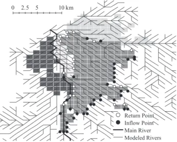
The water allocation scheme simulates water diversion at the weirs, followed by its allocation to the associated irrigated areas. The estimated amount of diverted water Qi (m³/dt) is allocated among the modeled irrigation systems along the flow pathways of the irrigation channel networks as described below. Thus, the amount of diverted water is calculated independently of the surface water flows in the runoff module. In the base model, the diverted water is supplied to paddies within the same grid cell, but the new model can simulate water allocation across multiple grid cells.

(1) Extraction of irrigation networks using GIS data- base

To model water fluxes across large irrigated areas, precise data describing water use facilities and channel networks are needed. These data were obtained from a recently configured GIS database of water use facilities throughout Japan (Japan Institute for Irrigation and Drainage, 2010; data acquired on 2014.5.12). This database includes specifications for irrigation facilities, irrigation channel networks, and irrigation block polygons;

the latter two have rarely been incorporated into hydrological models.

The database includes water use facilities (diversion weirs, drainage pumps, and reservoirs) and irrigation and drainage channels that serve an area exceeding 100 ha; the former are represented by point data and the latter by line data. These data have attributes of function and name, and they can be separated or grouped according to their connectivity. However, the database lacks information necessary to link the vector (i.e., point and line) data to the polygon (areal) data of the irrigation blocks. Therefore, an algorithm was developed to link the vector and polygon data for simulation of water allocation to irrigated areas. The algorithm is implemented in two steps. First, an irrigation network is created by linking water diversion facilities (point data) to irrigation channels (line data). Second, the irrigation network is overlaid on the irrigated blocks (polygon data) to link the diversion facilities with their associated irrigated areas. In this way, the spatial extent of each irrigation system is determined, and water allocation to each irrigation area can be simulated.

(2) Water diversion and allocation schemes

First, the amount diverted daily at each diversion weir Qi is determined as the minimum value among the fol-

(12)

Water Intake Q_i

Precipitation p

Irrigation Supply to Paddies Q_a Paddies

ET Infiltration Surface Runoff River Flow Water Loss

during Allocation Q_dr Allocated Water

to Grid-cell Q_gw lowing: daily river discharge Qch(m³/dt), designed maxi-

mum intake capacity Qif(m³/dt), and the water requirement of the associated irrigation areaQgw(m³/dt).

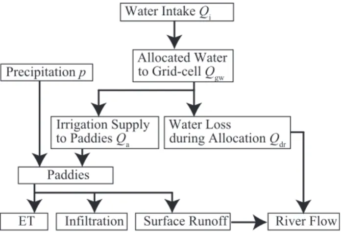
Then, Qi is allocated by dividing it into irrigation water supplied to paddies and management water loss (i.e., the management water requirement). The management water loss, which consists of water that does not reach the irrigated area (paddy fields), gradually returns to streams. In the paddy fields, the irrigation supply is divided into percolation, runoff from fields, and ET. The management water requirement and runoff from paddy fields are passed to the surface runoff module.

The water allocation calculation is independent of the surface runoff calculation. In the runoff module, the flow direction in each grid cell depends on the local topography and the stream flow direction, but in the water allocation scheme, water flow to irrigated areas follows the irrigation channel network. Therefore, the model simulates water allocation to the irrigation areas according to the priority order of the grid cells composing each irrigated block of paddies (here, an irrigated block can be represented by multiple grid cells or by a single grid cell). Paddies in a grid cell in the upper part of an irrigation block that is directly connected to an irrigation channel have a higher priority than those in a grid cell in the lower part of a block that is not directly connected to a channel. Thus, the priority order of each grid cell is determined by 1) its distance from the diversion weir, 2) its distance from an irrigation channel, and 3) its elevation. Water is then allocated to each grid cell following its priority order in the irrigation block according to the water demand in that grid cellQgw.

The gross irrigation water requirement (mm/d) (i.e., the amount of water that must actually be extracted from the diverted water) is computed by dividing the net irrigation requirement by the irrigation efficiency Ie, which represents the water loss during the distribution and application of the water to the paddies.

Repetitive use of water within irrigated blocks is not accounted for in this model, and irrigation and drainage channels are assumed to be separate. Hence, the total Qgwin an irrigated area may exceed the diverted amount Qi, depending on the available river flow. In this case, water is not allocated to grid cells with a low priority order.

Qgw consists of allocated water Qa(m³/dt)(= QrqAir/ 1,000) and water loss during allocation Qdr(m³/dt) (Fig. 4). Water lost during allocation returns to the drainage channels within a day (Sato et al., 1998); thus, Qdris added to the lateral inflow into drainage channels on the day following the allocation. If the sum of water

allocated to all irrigated grid cells in the irrigated block is less than the total amount of diverted waterQi, the re- mainder of the water is distributed equally to all grid cells in the irrigated block or added to the drainage channels via lateral inflow.

For irrigated blocks that consist of a single grid cell, the water diversion and allocation scheme is the same as that of the base model: that is, allocated water Qais determined as follows:

3.3 Study watershed

3.3.1 Topography, geology and climate of the study watershed

The Seki River basin in central Japan was selected for a case study. The Seki River is 64 km long, and its catchment area is 1140 km². The land cover is dominantly forest (79%), but 17% of the land area of the catchment is agricultural land, mainly rice paddies. The Seki River flows from the Myoko Mountains (highest peak, Myoko Mountain, 2425 m a.s.l.) to the Japan Sea (Figs.5, 6). Hillslopes are steep, and the bedrock is a mixture of various Tertiary sedimentary rocks, which are mantled by alluvium. The climate of the basin is humid, typical of the Japan Sea area, and snowfall is heavy in winter. Average annual precipitation is more than 3000 mm, over half of which falls as snow in winter.

3.3.2 Agricultural water use in the basin

The total irrigated area of the basin is approximately 9000 ha, and it is mostly used for rice paddies. There are two major irrigation systems on the eastern side of the Seki River (Fig. 6); the Uwae (approximately 2000 ha) and the Nakae (approximately 3000 ha) systems.

The Nakae diversion weir was originally located 3 km downstream from the Uwae diversion weir, which led to complex conflicts between the two systems when the conventional water use rule was applied, because Nojiri

Fig. 4 Schematic diagram of water flows in the water allocation scheme.

(13)

Meteo. Obs. point Elevation (m)

- 500 500 - 1,000 1,000 - 1,500 1,500 - 2,000 2,000 - 2,500 0 5 10 15 20 km

Flow Gauge (Futagojima) Sasagamine

Dam Shozenji Dam Flow Gauge (Takada)

Nojiri Lake Seki River Basin

Sea of Japan

Niigata Pref. Hokura River

Seki River

Flow Gauge (Arishima)

0 5 10 km

Sea of Japan Hokura R.

Seki R. Itakura DW Flow Gauge

(Takada)

Sekikawa DW

Kenshoji DW

Iida R.

Bessho R. Kushiike R.

Ookuma R.

Uwae IC Nakae IC Ohbuke IC Inarinakae IC Koyasu IC DW: Diversion Weir IC: Irrigation Canal R: River Yashiro R.

Koyasu DW

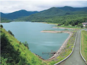
Lake (effective storage for irrigation: 9.8 × 10⁶m³), one of the major irrigation reservoirs, is controlled by the Nakae system. However, the construction of Sasagamine dam 9.2 × 10⁶m³,Fig. 7) and the Itakura diversion weir (Fig. 8), which now serves both systems, resolved these conflicts (Shinzawa, 1962). Currently, the Itakura diversion weir not only diverts and allocates water to both the Uwae and Nakae irrigation systems, it also diverts water for hydropower generation. Other irrigation systems shown in (Fig. 6) include the Inari-Nakae system on the western side of the Seki River (approximately 600 ha) and the Ohbuke irrigation system along the Ho- kura River (approximately 1600 ha). Shozenji dam (effective storage 4×10⁶m³, Fig. 5) stores water for domes- tic use.

3.3.3 Collected data and data input procedures For the model application, the Basic Grid Square (Third Area Partition) of the Standard Regional Mesh Code was used for the grid. In this system, each grid cell covers 45 seconds of arc in the longitudinal direction and 30 seconds of arc in the latitudinal direction, and in central Japan its area corresponds to approximately 1 km². Elevation and land use/cover data for each grid cell were obtained from the National Land Numerical Information website of the Ministry of Land, Infrastructure and Transportation (data acquired on 2014 /09/20) and the GIS database of water use facilities in Japan (Japan Institute for Irrigation and Drainage, data acquired on 2014/05/12). The steepest descent method was used to determine the water flow direction in each grid cell, and the direction of river flow in a grid cell was toward the lowest grid cell among the eight neigh- boring grid cells.

Required meteorological data (precipitation, temperature, humidity, and wind speed) were collected from

Fig. 7 Photograph of Sasagamine dam looking west. See Fig. 5 for its location.

Fig. 5 Location of the Seki River basin (inset), and locations of hy- drometeorological observation points in the basin. The grid applied to the study area and its topography are also shown.

Fig. 8 Photograph of the Itakura diversion weir looking upstream (north). See Fig. 6 for its location.

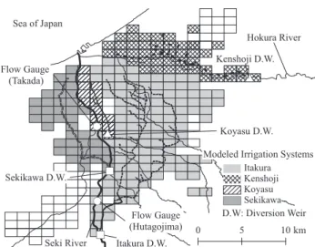
Fig. 6 The major irrigation facilities in the areas served by the Land Improvement Districts of the lower Seki River basin. Differ- ent irrigation areas are shown by different hatching patterns and gray shading.

(14)

0 5 10 km Sea of Japan

Hokura River

Seki River Itakura D.W.

Sekikawa D.W.

Kenshoji D.W.

Modeled Irrigation Systems Itakura Kenshoji Koyasu Sekikawa Koyasu D.W.

D.W: Diversion Weir Flow Gauge

(Hutagojima) Flow Gauge

(Takada)

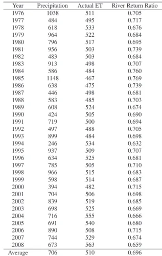
1976 through 2008 at existing observation stations (Fig. 5). The meteorological data were obtained from the database of the Automated Meteorological Data Ac- quisition System (Japan Meteorological Agency), the River Bureau of Ministry of Land, Infrastructure and Transport, and the Myoko-Sasagamine Station of the National Institute for Earth Science and Disaster Preven- tion. To estimate the spatial variation in the observed meteorological variables, the inverse distance weighting method was employed. In this method, the grid cell values are determined by calculating the weighted average of values observed at observation stations in the neigh- borhood of each grid cell. The closer a station is to the center of the cell being estimated, the greater its weight in the averaging.

Precipitationp(x) (mm/d) in grid cellx was estimated by calculating the average of data from three observation stations, weighted according to the distance from x to the observation station. Then, the ratio of the observed precipitation to the estimated climatic value r(i) (where i = 1, 2, 3) in the grid cell of station i was calculated as follows:

where po(i) (mm/d) is the observed precipitation at station i and pm(i) (mm/d) is the climatic value derived from Mesh Climatic Data 2000, which is the monthly climatic precipitation for the corresponding Basic Grid Square (Third Area Partition) estimated from the observed spatial distribution of rainfall from 1971 through 2000 (Japan Meteorological Agency, 2003).

Then, ratio r(i) is interpolated to each grid square of the model by using the inverse distance weighting method as follows:

where d(i) is the distance from grid cell x to observation stationi.

Finally,p(x) is estimated by multiplyingr(i) bypm(i).

Ideally, the estimated grid cell x should be located within a triangle formed by the three observation points;

however, the same procedure was applied for grid cells outside of such a triangle. Snowfall and snowmelt processes, which were also incorporated in the precipitation estimation, are described in Section 4.. The values of other meteorological variables used for ET estimation were similarly interpolated by using the inverse distance method.

River discharge, which was observed at Takada and Futagojima flow gauge stations (Fig. 5) from 2003 through 2008, was used to validate the model. The upstream station (Futagojima) is located immediately

downstream of the largest diversion weir, and the downstream station (Takada) is located near the basin outlet.

The recorded data at both stations were affected by both water diversion and return flow.

Actual ET, calculated by the method proposed by Ohtsuki (1984), was used for the adjustment of the root zone storage Srmax so that the actual ET calculated with equation (17) (see Section 2) would equal the Actual ET value. Then, the annual water balance at Takada station was calculated, and areal precipitation was corrected to satisfy the water balance of the watershed.

3.3.4 Settings for the water allocation and management module

To apply the water allocation and management module, 16 irrigated blocks were delineated in the watershed by the method described in Section 2. Three major irrigation blocks, for which water is diverted at the Itakura, Sekikawa, and Kenshoji diversion weirs, respectively, are shown inFig. 9.

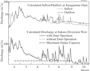
In the reservoir operation scheme, each reservoir needs to be linked to a diversion weir, so that the water released for irrigation can be estimated. Here, the Sasa- gamine dam reservoir is linked to the Itakura diversion weir, and Nojiri Lake is linked to the Sekikawa diversion weir. The maximum release from each reservoir for hydropower generation was set to 3.28m³/s based on the published operation rule (Niigata Prefecture, 1985).

The paddy outlet height was set to 30 mm, and the maximum infiltration rate at the paddy surface was set to 5 mm/d, based on survey data obtained by the Ho- kuriku Regional Agricultural Administration (1984).

Planting starts when the allocated water is greater than 120 mm, which is the water requirement for irrigation planning in this region, and the cropping period was set to 100 days.

Fig. 9 The modeled irrigated areas and their associated irrigation facilities in the lower Seki River basin.