線形計画法を用いた区間解析(科学技術における数値計算の理論と応用II)

線形計画法を用いた区間解析

山村清隆

群馬大学工学部情報工学科

群馬県桐生市天神町

1-5-1

あらまし 区間解析は非線形方程式のすべての解を求める代表的な方法として知られてい るが, 問題の次元の増加とともに計算時間が指数関数的に増大する欠点をもつ

.

区間解析の 計算効率を改善するためには, 与えられた領域に解が存在しないことを判定する強力なテスト を開発する必要がある

.

本論文では

,

区間解析に線形計画法を導入することにより

,

線形項の

多い非線形方程式に対しては, そのすべての解を非常に効率よく求められることを示す.

本手 法の基本的な考えは次の通りである

.

まず与えられた領域に対し

,

区間拡張を用いて非線形関 数を長方形 (あるいは多次元の直方体) で囲み, その領域内のすべての解を含むような実行可 能領域をもつ線形計画問題を定式化する

.

そのような実行可能領域の存在非存在を単体法の

Phase I

で確認することにより, 非線形方程式の解の非存在を判定することができる

.

さらに

Phase II

を利用して実行可能領域を含む最小の直方体を求めることにより

,

同じ解を含むより 小さな領域を得ることができる

.

このテストは従来の区間解析で用いられているテストよりも 遥かに強力で, 区間解析の計算効率を飛躍的に改善することができる

.

Interval Analysis

Using Linear Programming

Kiyotaka

YAMAMURA

Department

of Computer Science, Gunma University, Kiryu 376, Japan

$\mathrm{E}$

-mail:

[email protected]

Tel:

0277-30-1812

Fax:

0277-30-1814

Abstract A

new

computational

test is proposed for nonexistence of

a

solution to

a

system

of

nonlinear equations in

a

convex

polyhedral

region

$X$

.

The

basic

idea proposed here

is

to

formulate

a

linear

programming

problem whose

feasible

region

contains

all

solutions

in

X. Therefore, if the

feasible

region

is empty

(which

can

be easily checked by Phase I

of

the

simplex

method),

then the system

of

nonlinear equations has

no

solution in

$X$

.

The

linear

programming

problem

is

formulated

by surrounding the component nonlinear functions

by

rectangles using interval extensions. This test is much

more

powerful

than

the conventional

test if the

system

of nonlinear

equations

consists of

many

linear terms

and

relatively

a

small number of nonlinear terms.

By

introducing the

proposed

test

to

interval

analysis,

all

solutions

of

nonlinear equations

can

be

found very

efficiently.

1. Introduction

This paper deals with the problem of finding all solutions ofa system of nonlinear equations:

$f_{1}(_{X_{1}}, X_{2,,n}\ldots X)$ $=$ $0$ $f_{2}(X_{1}, X_{2,n}\ldots, X)$ $=$ $0$ (1)

.

$\cdot$

.

. $f_{n}(x_{1}, x_{2,n}\ldots, X)$ $=$ $0$

containedin a bounded rectangular region$D$in$R^{r\mathrm{r}}$, where $f_{1},$ $f_{2},$_$\cdots,$$f_{n}$ are real-valued nonlinear

func-tions. In vector notation the system (1) will be written as $f(x)=0$.

As a computational method to find all

solu-tions of nonlinear equations, interval analysis is well-known, and various algorithms based on in-terval computation have been developed $[1],[2],[5]-$

$[19],[23]-[28],[30]$

.

Using the interval analysis, all

solutions of (1) contained in $D\subset R^{n}$ can be found

with mathematical certainty. However, the compu-tation time of the interval analysis tends to grow

exponentiallywith thedimension$n$

.

Evenfor small

problems, the interval analysis often requires enor-mous computation time if the nonlinearity of the problems is very large or the problems are ill-conditioned.

In order to improve the computational effi-ciency of the interval analysis, it is necessary to develop a powerful method for excluding interval vectors ($n$-dimensional rectangules) containing no

solution very effectively. In this paper, we propose a new computational test fornonexistence ofa so-lution tothe system ofnonlinearequations (1) in a region$X$

.

The basic ideaproposedhereisto

formu-late a linear programming problem whose feasible region contains all solutionsin$X$

.

Hence, if the

fea-sible region is empty (which can be easily checked by Phase I of the simplex method), then $X$

con-tainsnosolution,andwe canexcludeit from further consideration. The linearprogramming problem is formulated by surrounding the component nonlin-ear functions by rectanglesorsuitableconvex

poly-go.ns.

This test is

_{much.morep-owerful}

than the conventional test if the system of nonlinear equa-tions consists ofmany linear terms and relatively a small number of nonlinear terms. By numerical ex-amples, it is shownthat all solutions can be found very efficiently by using the proposed test.

Most of the theoretical results of this paper have been presented in $[36]-[381\cdot$ This workis an

extension of the ideas in [21] and [40] to finding all solutions ofnonlinear equations.

2. Interval Analysis

In this section, we summarize the basic procedure oftheinterval analysis briefly.

Intervals will be denoted by capital letters. An $n$-dimensional interval vector with components

$x_{i}--[a_{i},$$b_{i}$

}

$(i=1,2, \cdots , n)$ is denoted by

$X=(_{-\lambda_{1}^{r},x}2, \cdots,X_{n})T$

.

(2)

Geometrically, $X$is an$n$-dimensional rectangle.

In the interval analysis, the following proce-dure is performed recursively beginning with the initial region $X=D$

.

Ateach level,we analyze the region $X$

.

Ifthere is no solution of (1) in $X$, then

we exclude it from further consideration. If there is a uniquesolution of (1)in$X$, thenwecomputeitby

some iterativemethod. In the field of interval anal-ysis, computationally verifiable sufficient conditions fornonexistence, existence and uniqueness ofa so-lutionin$X$have been developed. If these conditions

are not satisfied

_and.the

existence or nonexistence ofa solution in$X$cannot be$\mathrm{c}\mathrm{h}\mathrm{e}\mathrm{C}\mathrm{k}\mathrm{e}\dot{\mathrm{d}}$

,then bisect$X$

in some appropriately chosen coordinate direction to form two new rectangles; we then continue the above procedure with one of these rectangles, and

put the otherone on astack forlater consideration. The nonexistence of a solution in $X$ can

be checked by using interval extensions. If in

$f(x_{1,2,n}x\cdots, x)$ the variables $x_{i}$ are replaced by

intervals $X_{i}$ and the alithmetic operations are

re-placed by the corresponding interval operations (for

example, $x_{1}+x_{2}$ is replaced by _{$X_{1}+X_{2}=[a_{1}+$}

$a_{2},$$b_{1}+b_{2}])$, then an interval-valuedvector function

$F(X)$ is_{obtained which} is_{called theinterval}

exten-sion of $f(x)$. It is known that $F(X)$ contains the

rangeof $f(x)$ over $X$

.

Hence, if

$0\not\in F(X)$ (3)

holds, then there is no solution of(1) in$X$. This is

the computationally verifiable sufficient condition fornonexistence ofa solution to (1) in $X$, whichis

usedasthetest fornonexistenceintheconventional interval analysis $\dagger$

.

Geometrically, (3) implies that there exists an

$\dot{i}$ such that the

$(n-1)$-dimensional solution sur-face satisfying $f_{i}(x)=0$ does not exist in $X$

.

In

other words, if all solution surfaces of $f_{i}(X)=0$ $(i=1,2, \cdots, n)$ exist in $X$, then _{$0\in F(X)$} holds.

However, although all solution surfaces exist in $X$,

asolutiondoesnotexist unless theyintersect at the samepoint. Hence, $\mathrm{O}\in F(X)$ is merelya necessary

condition for existence of solutions in $X$

.

In

prac-tical applications, $0\in F(X)$ often holds although

there is no solution in $X$, especially when the

rect-angle $X$ is large or $f(x)$ is ill-conditioned. _Thus,

(3) is not necessarily a powerful test for excluding

\dagger As _{another computationally verifiable sufficient}

condition for nonexistence ofa solution to (1) in $X$,

$K(X)\cap X=\phi$ _{is known where}$K(X)$ is the Krawczyk

regions. In order to improve the computational ef-ficiencyof the interval analysis, it is very important to develop a powerfultest which checks the nonex-istence ofa solutionin $X$

.

3. A New Test Using Linear Programming 3.1 Basic Idea

In practical problems, the system of nonlinear equa-tions often consists of many linear terms and rela-tively a small number of nonlinear terms. The test proposed in this paper is suited to such systems. In this section, we first consider the casewhere (1) can be represented as

$\sum_{i\in J_{i}}gii(X_{j})+\sum_{j=1}^{n}$

hijxj–si

$=0,$ $i=1,2,$$\cdots,$$n$

(4) where$g_{ij}(x_{j})$isanonlinear function ofonevariable,

$h_{ij}$ and $s_{i}(i, j=1,2, \cdots, n)$ are constants, and $J_{i}$ is asubset of $\{$1, 2,$\cdots$,$n\}$

.

Assume that $\sum_{i=1}^{n}|J_{i}|$

is not a so largenumber,where $|J_{i}|$denotesthe

car-dinality of the set $J_{i}$

.

The case where nonseparable

functions ofmore than one variables are contained will be considered later. As a typical example of the system of nonlinear equations of the form (4), nonlinearcircuit equations inhybridrepresentation [4], [35] is known, where$J_{i}=\{i\}$ holds for all $\dot{i}$

.

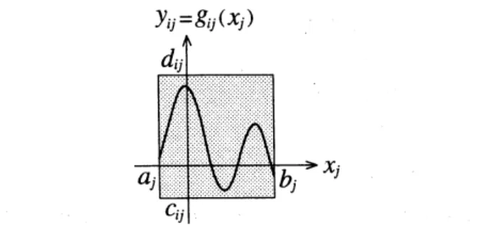
Let therangeof$g_{ij}(x_{j})(i=1,2, \cdots, n, j\in J_{i})$

over $[a_{j}, b_{j}]$be$[c_{ij}, d_{ij}]$. Here, therangemay be the

exact range (if possible) or the interval extension containing the exact range. Then, we introduce auxiliary variables $y_{ij}$ $(i=1,2, \cdots, n, j \in J_{i})$

and put $y_{ij}=g_{ij}(X_{j})$. If $a_{j}\leqq x_{j}\leqq b_{j}$, then

$c_{ij}\leqq y_{ij}\leqq d_{ij}$

.

Nowweconsider the following linear program-ming $(\mathrm{L}\mathrm{P})$ problem:

$\max$ (arbitrary function)

subject to

$\sum_{j\in J}.\cdot yij+\sum_{j=1}^{n}h_{ij^{X_{j}}}-s_{i}=0$, $i=1,2,$$\cdots,$$n$

$a_{i}\leqq x_{i}\leqq b_{i}$, $i=1,2,$$\cdots,$$n$ $c_{ij}\leqq y_{ij}\leqq dij$, $i=1,2,$$\cdots,$$n$,

$j\in J_{i}$

.

$(5)$

Geometrically, the inequality

constraints

in (5) implies that the component nonlinear functions

$gij(Xj)$ are surrounded by rectangles as shown in

Fig. 1.

$\mathrm{E}\mathrm{v}\mathrm{i}\mathrm{d}\mathrm{e}\dot{\mathrm{n}}\mathrm{t}\mathrm{l}\mathrm{y}$, all solutions of (4) which exist in

$X=([a_{1,1}b], \cdots, [a_{n}, b_{n}])^{\tau}$ satisfy the constraints

Fig. 1 $\ln$the proposedtest, nonlinear functionsare

sur-rounded by rectangles.

in (5) if we put $y_{i\mathrm{j}}=g_{ij}(x_{j})$. Namely, the feasible

region of the LP problem (5) is a convex polyhe-dron containingallsolutions of (4) in $X$

.

Hence, if

the feasible region is empty, then we can conclude that there is no solution of (4) in $X$

.

The emptiness or nonemptiness of the feasible region of (5) can be checked by Phase I of the sim-plex method $\dagger$

.

This is the new computational test for nonexistence of a solution to (4) in $X$

.

This

test is very simplebecause we just apply Phase I of the simplex method to (5). Since there are many good softwares of the simplex method, the imple-mentation of the proposed test is very easy. For simplicity, we will refer to the proposed test as the LP test.

Note that if the feasible region is empty, then any system of nonlinear equations of the form (4) where therange of$gij(x_{j})$ $(i=1,2, \cdots , n, j\in J_{i})$

over $[a_{j}, b_{j}]$is contained in $[c_{ij}, d_{ij}]$doesnot have a

solution in $X$

.

Asshowninthefollowingexample, theLPtest is more powerful (often much more powerful) than the conventional test (3). This is because the

struc-ture of (4) is fully exploited in the new test. Example: Consider a system of nonlinear equa-tions:

$f_{1}(x_{1},$$X_{2}\mathrm{I}=x_{1}-x_{2}=0$

$f_{2}(X_{1}, x_{2})=(x_{1}-1)^{2}-x_{2}=0$

.

Let $X=([-10,0], [-10,10])T$

.

Using the exact range, we obtain $F(X)=([-20,10], [-9,131])^{T}$

.

Since $0\in F(X)$, the conventional test (3) cannot

exclude this region. However, since the feasible

re-$\frac{\mathrm{g}\mathrm{i}\mathrm{o}\mathrm{n}\mathrm{S}\mathrm{a}\mathrm{t}\mathrm{i}\mathrm{S}\mathrm{f}\mathrm{y}\mathrm{i}\mathrm{n}\mathrm{g}}{\mathrm{t}\mathrm{T}\mathrm{h}\mathrm{i}\mathrm{S}\mathrm{i}\mathrm{d}\mathrm{e}\mathrm{a}\mathrm{i}\mathrm{s}\mathrm{a}\mathrm{n}\mathrm{e}\mathrm{X}\mathrm{t}\mathrm{e}\mathrm{n}\mathrm{s}\mathrm{i}\mathrm{o}\mathrm{n}\mathrm{o}\mathrm{f}\mathrm{t}\mathrm{h}\mathrm{e}\mathrm{i}\mathrm{d}\mathrm{e}\mathrm{a}\mathrm{s}\mathrm{i}\mathrm{n}[21]\mathrm{a}\mathrm{n}\mathrm{d}}$

[40] to finding all solutions of nonlinear equations. In [21],the concept ofpolyhedral circuit (i.e., circuitwith resistive elements whose characteristics are polyhedra)

is introduced andtheemptiness or nonemptiness of the solution domain of the polyhedral circuit is checked by Phase I of the s\’implex method. In [40], anLP problem similar to (5) isformulated for finding all solutions of piecewise-linear circuits.

$x_{1}-x_{2}=0$ $y_{1}-x_{2}=0$

$-10\leqq X_{1}\leqq 0$ $-10\leqq x_{2}\leqq 10$

$1\leqq y_{1}\leqq 121$

isempty, theLP test can exclude this region. $\square$

Now let us examine the size ofthe tableau in the LP test. In the implementation of the simplex method to (5), we _{apply the variable} transforma-tion $\overline{x}_{i}=x_{i}-a_{i}$ and $\overline{y}_{ij}=y_{ij}-c_{ij}$ so that the

LP problem becomes the form with nonnegativity constraints:

$\max$ (arbitrary function)

subject to

$\sum_{j\in j}.\cdot\overline{y}_{ij}+j=\sum hij\overline{x}j-\overline{s}_{i}=01n$, $\dot{i}=1,2,$$\cdots,$$n$

$\overline{x}_{i}\leqq b_{i}-a_{i}$

,

$i=1,2,$

$\cdots,$$n$

$\overline{y}_{ij}\leqq d_{ij}-C_{ij}$, $i=1,2,$_{$\cdots,$$n,$} $j\in J_{i}$

$\overline{x}_{i}\geqq 0$, $\overline{y}_{ij}\geqq 0$, $i=1,2,$

$\cdots,$$n,$ $j\in J_{i}$

.

(6) This LP problem has $n$ equality constraints and

$\sum_{i=1}^{n}(l_{i}+1)$ inequality constraints (excluding the

nonnegativity constraints) where $l_{i}=|J_{i}|$

.

In-troducing the slack variables $\lambda_{i}$ and $\mu_{ij}(\dot{i}$ $=$

$1,\mathit{2},$$\cdots$,_$n,$ $j\in J_{i}$), (6) is transformed into a

stan-dard form:

$\max$ (arbitrary function)

subject to

$\sum_{j\in j}\dot{.}\overline{y}_{ij}+j=\sum hij^{\overline{X}}j-\overline{s}i=01n$, $i=1,2,$_$\cdots,$$n$

$\overline{x}_{i}+\lambda_{i}=b_{i}-ai$, $i=1,2,$

$\cdots,$$n$

$\overline{y}_{ij}+\mu_{ij}=dij-Cij$, $i=1,2,$_{$\cdots,$$n,$} $j\in J_{i}$

$\overline{x}_{i}\geqq 0$, $\overline{y}_{ij}\geqq 0$, $\lambda_{i}\geqq 0$, $\mu_{ij}\geqq 0$,

$i=1,2,$$\cdots,$$n,$ $j\in J_{i}$

.

In Phase I, we introduce artificial variables to ob-tainaninitial basicfeasiblesolution. Since $b_{i}-a_{i}>$

$0$and_{$d_{ij}-c_{ij}>0(\dot{i}=1,2, \cdots, n, j\in J_{i})$} hold,we

only need to introduce $n$ artificial variables for the

first $n$ equality

constraints.

Hence, the

size

of the

tableauis $\{\sum_{i=1}^{n}(l_{i}+2)+1\}\cross\{\sum_{i=1}^{n}(l_{i}+1)+1\}$

.

Remark1: The LP testcanbe applied to thecase where$X$ isaconvexpolyhedron _{otherthan a}

rect-angle. In that case, wereplace $a_{i}\leqq x_{i}\leqq b_{i}(\dot{i}=$

\a ノ $1^{\cup}J$

Fig. 2 Nonlinear functions surrounded by right-angled

triangles.

1, 2,$\cdots$

’$n$) in (5) by the inequalities $\mathrm{r}\mathrm{e}\mathrm{p}\mathrm{r}\mathrm{e}\mathrm{s}\mathrm{e}\mathrm{n}\mathrm{t}\mathrm{i}\mathrm{n}_{\square }\mathrm{g}$

the region $X$

.

Remark 2: In the LP test, the component non-linear functions $gij(Xj)$ _{are surrounded by}

rectan-gles as shown in Fig. 1. However, if the component nonlinear functions have some favorable properties suchas monotonicity or convexity, then we may

sur-round thembysuitable convexpolygons instead of

the rectangles. Forexample, if thefunctions$g_{ij}(x_{j})$

are monotone and convex, then it is efficient to

surroundthem byright-angled triangles whose two sides areparallelto the$x_{j}$ and $y_{ij}$ axes asshownin

Fig. 2. In the case ofFig. $2(\mathrm{a})$, weapply the

vari-able transformation $\overline{x}_{j}=b_{j}-x_{j}$ and $\overline{y}_{ij}=y_{ij}-cij$,

and in the case of Fig. $2(\mathrm{b})$, we apply the variable

transformation $\overline{x}_{j}=x_{j}-a_{j}$ and $\overline{y}_{ij}=d_{ij}-y_{ij}$.

Then,wecanrepresent the right-angled triangleby

one inequality constraint:

$\overline{y}_{ij}\leqq-\frac{d_{ijj}-C_{i}}{b_{j}-a_{j}}\overline{X}_{j}+(d_{iij}j-C)$ $(\overline{(})$

and the nonnegativity constraints $\overline{x}_{j}\geqq 0$and $\overline{y}_{ij}\geqq$

$0$

.

Hence, the number of inequality constraints

de-creases compared with (6). Moreover, since trian-gles are smaller than rectangles, the LP test be-comes more powerful by using right-angled trian-gles. However, ifweuse triangles other than right-angled triangles, then the computation time often becomes larger because the

$\mathrm{n}\mathrm{u}\mathrm{m}\mathrm{b}..\mathrm{e}\mathrm{r}$

of.

$\mathrm{i}\mathrm{n}\mathrm{e}\mathrm{q}\mathrm{u}\mathrm{a}\mathrm{l}\mathrm{i}\mathrm{t}\Pi \mathrm{y}$

constraints increases.

3.2 Application to More General Cases

The LP test can be applied to the case where the system of nonlinear equations (1) contains nonsep-arable functions of more than one variables. For example, as

sume

that (1) contains a nonseparable function oftwo variables $g(x_{1}, x_{2})$

.

In this case, we

first compute the range of$g(x_{1}, x_{2})$ over $X$ by

in-terval operations. Let the range be $[c, d]$

.

Then,

we introduce an auxiliary variable $y$ $-g(x_{1,2}x)$

$g(x_{1}, x_{2})$ is replaced by $y$ and the inequality

con-straint$c\leqq y\leqq d$is added. That is, wesurroundthe

two-dimensional function surface of $y=g(x_{1}, x_{2})$

by a three-dimensional rectangle. Such extension is also possible to more general cases; if (1) con-tains a nonseparable function of $m$ variables, then

we surround the$m$-dimensional function surface by

an $(m+1)$-dimensional rectangle. Then, we can

formulate the LP problem similar to (5).

Example: Let $X=([1,2], [1,2])^{T}$ _{and considera}

system of nonlinear equations:

$f_{1}(X_{1,2}X)=x_{1}-x_{2}=0$

$f_{2}(x_{1}, x_{2})=x_{1}x_{2}-4X_{1}+2x_{2}-3=0$

.

Then, the LP problem we consider is

$\max$ (arbitrary function)

subject to $x_{1}-x_{2}=0$ $y-4x_{1}+2x2-3=0$ $1\leqq x_{1}\leqq 2$ $1\leqq x_{2}\leqq 2$ $1\leqq y\leqq 4$

.

In this problem, the feasible regionis empty. $\square$

Remark 3: It is known that any nonseparable function ofmany variablescan berepresented by a

set of separable functions, $\mathrm{i}.\mathrm{e}.$, additions of

func-tions of one variable $[33],[34],[39]$

.

For example,

$\exp(2x_{1}+x_{1}x_{2}+3x_{3}^{2})$ can berepresented as $\exp(2_{X_{1}}+x_{1}x_{2}+3x_{3}^{2})$

$arrow$ $\exp(Z_{1})$

$z_{1}=2x_{1}+(z_{212}^{2}-X^{22}-X)/2+3x_{3}^{2}$ $z_{2}=x_{1}+x_{2}$

where$z_{1}$ and $z_{2}$ are auxiliary variables. Algorithms

forrepresenting nonseparable functions by separa-blefunctions are proposed in $[33],[34]$

.

Ifwe

repre-sent the nonseparable functions in (1) by separable functions, then we can perform the

_L.

$\mathrm{P}$ test

$\mathrm{u}\mathrm{s}\mathrm{i}\mathrm{n}\mathrm{g}\square$

$\mathrm{t}\mathrm{w}\mathrm{o}^{-}\mathrm{d}\mathrm{i}\mathrm{m}\mathrm{e}.\mathrm{n}\mathrm{s}\mathrm{i}0\mathrm{n}\mathrm{a}1$ rectangles only.

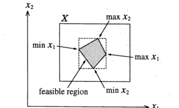
3.3 FindingSmallerRegionsContainingtheSame Solutions Using PhaseII

In the LP test, the emptiness or nonemptiness of the feasible region is checked by Phase I of the simplex method. If it is not empty, then we find a basic feasible solution (an extreme point of the feasible region) at the end of the Phase I. Then,we may solve the following$2n$ LP problems:

Fig. 3 The smallest rectanglecontainingthe feasibleregion

can be obtained by Phase11.

$\max/\min x_{k}$

subject to

$j \in J\sum_{i}y_{i}j+\sum_{j=1}^{n}h_{ij}Xj-si=0$, $i=1,2,$$\cdots,$$n$

$a_{i}\leqq X_{i}\leqq b_{i}$, $i=1,2,$

$\cdots,$ $n$

$c_{ij}\leqq y_{ij}\leqq dij$, $i=1,2,$$\cdots,$$n$,

$j\in J_{i}$

for $k=1,2,$$\cdots,$$n$

.

That is, we maximize and

min-imize $x_{k}$ for all $k=1,2,$$\cdots,$$n$under the same

con-straints as those in (5). Since we have already ob-tained the basic feasible solution by Phase I, these LP problems can be solved by Phase II only. As shown in Fig. 3.3, the optimal solutions of these

problems give the upper bounds and the lower

bounds of the feasible region ineach coordinate di-rection. Hence, we can obtain the smallest rectan-glewhich contains the feasibleregion (the rectangle described by dashed lines inFig. 3.3). Since all so-lutionsin$X$ are contained in this rectangle, we can

replace $X$ by this smaller region forimprovingthe

computational efficiency. Thus, the LP test can be used notonly to check thenonexistenceofa solution in$X$butalso to find a smallerregion containingthe

same solutions.

4. Numerical Examples

We introduced the LP test to the well-known Krawczyk-Moore algorithm $[12]-[15]$ and imple-mented the new algorithm (where the LP test is

performed after the test (3)$)$ using the program-ming language $\mathrm{C}$ on a Sun Ultra SPARC model

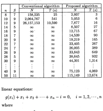
170. In the programming, weused the program of the simplex method written in [22]. We did not introduce the technique described in Section 3.3. We have applied the algorithm to many examples and have confirmed the large effectiveness of the LP test. In this section, weshow some examples. Example 1: We first considera system of$n$

non-Table 1 Resultofcomputation(Example1). Table 2 Result ofcomputation (Example 2).

linear equations:

$g(x_{i})+x_{1}+x_{2}+\cdots+x_{n}-\dot{\iota}=0$, $\dot{i}=1,2,$$\cdots,$$n$

where

$g(x_{i})=2.5x_{i}^{3}-10.5X_{i}^{2}+11.8x_{i}$

whichdescribesanonlinearresistive circuit contain-ing $n$ tunnel diodes $[31],[32],[35]$

.

We considered

theinitial region $([-10,10], \cdots, [-10,10])T$ and

ap-plied the conventional Krawczyk-Moore algorithm and the proposed algorithm for various $n$

.

Table 1

shows the result ofcomputation, where $S$ denotes

the numberof solutionsobtained by thealgorithms,

$N$ denotes the number of analyzed regions, $T$

de-notes the computation time, and $\infty$ denotes that

it could not be computed $\mathrm{i}\dot{\mathrm{n}}$

practical computation time. As seen from the table, the proposed algo-rithm is much more efficient than the conventional Krawczyk-Moore algorithm (especially when $n$ is

large).

Example 2: Wenext considerasystem of$n$

non-linearequations [3]:

$x_{i}- \frac{1}{2n}(\sum_{j=1}^{n}X^{3}j+i)=0$, $\dot{i}=1,2,$$\cdots,$$n$

.

The initial region is $([-10,10], \cdots, 1-10,10])^{\tau}$

.

We

applied the conventional Krawczyk-Moore algo-rithm and the proposed algorithm to this problem for various $n$

.

Table 2 shows the result of

com-putation. As seen from the table, the Krawczyk-Moore algorithm becomes much more efficient by introducing the LP test. It is also seen that the computation time of the proposed algorithm does not grow so explosively compared with that of the Krawczyk-Moore algorithm.

Example 3: We next consider a system of 10 equations:

$\sum_{j=1}^{10}X_{j}+x_{i}-(n+1)=0$, $i=1,2,$$\cdots,$$9$

$\prod_{i=1}^{10}xj-1=0$

which is known as Brown’s almost linear system

$[3],[8]$

.

The

initial region is $([-10,10], \cdots, [-10,10])T$

.

There are two solutions withinthe region.

Wen we applied the Krawczyk-Moore algo-rithm, the computation time was 375,804 seconds

(more than four days). However, when we applied

the proposed algorithm, all solutions werefound in

only 131 seconds.

Example 4: We next consider a system of$n$

non-linear equations:

$x_{i-1}-2x_{i}+x_{i+1}+h^{2}\exp(X_{i})=0$, $\dot{i}=1,2,$$\cdots,$$n$

where $x_{0}$ $=$ $x_{n+1}$ $=$ $0$ and $h$ $=$ $1/(n+1)$

.

This system comes from a nonlinear two-point boundary value problem termed the Bratu prob-lem [17]. Since the exponential function can be surrounded by a right-angled triangle, wealso con-sidered theLP test using right-angled triangles de-scribed in Remark 3.2. We considered the initial region $([-10,10], \cdots, [-10,10])T$ and applied the

Krawczyk-Moore algorithm and the proposed algo-rithms (i.e., theLP test algorithm using rectangles and that usingright-angledtliangles) for various$n$

.

Table3 shows the result of computation. It is seen that theBratu problem could be solved much more efficientlybyintroducing the LP test. It is also seen

that the LP test becomes more powerful by using right-angled triangles.

Example 5: Next, we consider the transistor-diodecircuit shown in Fig. 4 [29]. Usingthe Ebers-Moll model [4], thiscircuitis described byasystem of nonlinear equations in 15 variables of the form (4) where $J_{i}=\{i\}$

.

In this system, all nonlinear

$\prime_{-\mathrm{h}\mathrm{l}\mathrm{r}_{-}}.,\mathrm{t}l$ $\mathrm{D}arrow c$

”$1*-t’-\mathrm{m}-\mathrm{t}\mathrm{r}\star 0*:--’\varpi"-m-\mathrm{i}-\Lambda 1$

Fig. 4 Transistor-diodecircuit (Example 5).

Table 4 Resultofcomputation(Example 5).

functionsare the exponential functions. The initial region we consider is $([-20,0.5], \cdots, [-20, \mathrm{o}.5])^{\tau}$

.

There are 11 solutions within theregion.

We solved this system by the proposed algo-rithmusing rectangles, that using right-angled tri-angles, and that using triangles whose two sides are the tangents of$gij(Xj)$ at $(a_{j}, C_{i}j)$ and $(b_{j}, d_{ij})$

[37]. Table 4 shows the result of computation. It is seen that the LP test using right-angled tri-angles is the most efficient. This is because the number of inequality constraints decreases by us-ing right-angled triangles, and right-angled trian-gles are smallerthanrectangles. However, if we use triangles other thanright-angled triangles, the com-putation time often becomes larger although the number of analyzed regions decreases. This is be-causethe number of inequalityconstraintsincreases byusingtriangles other thanright-angled triangles. Example 6: Finally, we consider the transis-tor circuit shown in Fig. 5 [32], [39], [40] and the transistor-diode circuit shown in Fig. 6. The numbers of variables are 8 and 22, respectively.

Fig. 5 Transistor circuit (Example6).

Fig. 6 Transistor-diodecircuit (Example6).

Table 5 Result ofcomputation(Example6,$n=8$).

Table 6 Result of computation(Example6,$n=22$ ).

$[-20,0.5])T$

.

The numbers of solutions within the

region are 9and 1, respectively.

We solved this system by the proposed algo-rithmusing rectangles, that usingright-angled tri-angles, and that using triangles whose two sidesare thetangents of$g_{ij}(x_{j})$ at $(a_{j}, c_{ij})$ and $(b_{\mathrm{j}}, d_{ij})$

.

Ta-ble 5 and Table 6 showthe result of computation. In both cases,the LPtest usingright-angled trian-gles is the most efficient.

Remark 4: Recently, Prof. Shin’ichi Oishi of WasedaUniversity, Tokyo,Japan, succeeded to find all solutions of the multiphase equilibrium prob-lemof polymer solution (whichis a very important problem in polymer chemistry) by the Krawczyk-Moorealgorithmusingthe LP test [20]. This prob-lem is known to be a very difficult problem whose all solutions had not been found with mathematical certainty. In fact, this problem could not be solved by the conventional Krawczyk-Moore algorithm \dagger.

In [20], it is reported that all solutions of the

mul-tiphase equilibrium problem could be found with

guarant..eed

accuracy by using the algorithm

pro-posed in this paper and

the

numerical validation

system developed there [7]. - $0$

$5$

.

Conclusion

In this paper, a new computational test has been proposed for nonexistence of a solution to a sys-tem of nonlinear equations in a convex polyhedral region$X$

.

The basic idea proposed hereisto

formu-late a linear programming problem whose feasible region contains all solutions in $X$ (such a problem

can be formulated by surrounding the component nonlinear functions by rectangles) and then check the emptiness or nonemptiness of the feasible re-gion by the simplex method. The proposed test is very powerful if the the system of nonlinear equa-tions consists of many linear terms and relatively a small number of nonlinear terms. Moreover, it can be easily implemented because there are many publicly available softwares of the simplex method. Using the proposed test, we can find all solutions of nonlinear equations very efficiently.

Acknowledgement

Theauthors would like to thank Prof. Kazuo Hori-uchiand Prof. $\mathrm{S}\mathrm{h}\mathrm{i}\mathrm{n}’ \mathrm{i}_{\mathrm{C}\mathrm{h}\mathrm{i}}$ Oishi of Waseda University

for helpful discussions. They

are

also grateful to Prof. G\"otz E. Alefeld of Universit\"at Karlsruhe for

$\mathrm{t}_{\mathrm{I}\mathrm{n}}$ this problem, the

size of the regions on which the Krawczyk operator becomes contractive is less than $10^{-17}$

.

Hence, ifwe apply the Krawczyk-like _interyal algorithm, then the computation time and the memory space become impracticably large unless regions con-taining no solution are excluded very effectively.

kind advices. Thiswork was supported in part by

the Japanese Ministry of Education.

References

[1] G. Alefeld and J.Herzberger, lntroduction tolnterval

Computations,Academic Press, New York, 1983.

[2] G.Alefeldand J. Herzberger, “Aquadratically

conver-gent Krawczyk-likealgorithm,” SIAMJ. Numer. Anal., 20,pp.210-219, 1983.

[3] E. Allgower and K. Georg, “Simplicial and

continua-tionmethods forapproximatingfixedpointsand

solu-tionsto systems of equations”,SIAM Rev.,22,pp.

28-85, 1980.

[4] L. O. Chuaand P. M. Lin, Computer-Aided Analysis ofElectronicCircuits: Algorithmsand Computational Techniques, Prentice-Hall, Englewood Cliffs,New

Jer-sey, 1975.

[5] E. R. Hansen, “A globallyconvergent interval method

for computing and bounding real roots,” BIT, 18,

pp.415-424, 1978.

[6] E.R. HansenandS. Sengupta, “Bounding solutions of systemsofequationsusinginterval analysis,” $\mathrm{B}\mathrm{l}\mathrm{T},$$21$,

pp. 203-211, 1981.

[7] M. Kashiwagi and S. Oishi, “Numerical validation method for nonlinear equations using interval

anal-ysis and rational arithmetic,” IEICE Trans., J77-A,

pp. 1372-1382, 1994.

[8] R. B. Kearfott, “Some tests ofgeneralized bisection,”

ACM Trans. Math. Software, 13, pp. 197-220, 1987.

[9] R.B. Kearfott, Preconditioners for the interval

Gauss-Seidel method,” $\mathrm{S}\mathrm{l}\mathrm{A}\mathrm{M}.\mathrm{J}$. Numer. Anal., $27,$$,\mathrm{p}\mathrm{p}$. $804-$

$822$, 1990.

[10] R. B. Kearfott, “lnterval arithmetic techniques in the

$\mathrm{c}\mathrm{o}\mathrm{m}\mathrm{p}\mathrm{u}\dot{\mathrm{t}}\mathrm{a}\mathrm{t}\mathrm{i}\mathrm{o}\mathrm{n}\mathrm{a}\mathrm{l}$ solution

$0.\mathrm{f}$nonlinear systems of

equa-tions: Introduction, examples, and comparisons,” in

ComputationalSolutionof NonlinearSystems of Equa-tions(Lecturesin AppliedMathematics,Vol.26),E. L. Allgower and K. Georg,$\mathrm{e}\mathrm{d}\mathrm{s}.$,American Mathematical

Society,Providence, Rl, pp. 337-357,1990.

[11] R. B. Kearfott and V. Kreinovich, Applications of interval computations, Kluwer Academic Publishers,

Dordrecht, 1996.

[12] R. Krawczyk, “Newton-algorithmen zur bestimmung

von nullstellen mit fehlerschranken,” Computing, 4,

pp. 187-201,1969.

$.[13]$ R. E. Moore, “A test forexistenceof solutions to

non-linearsystems,” SIAM J. Numer. Anal., 14, pp.

611-615, 1977.

[14] R. E. Moore, Methods and Applications of

lnter-val Analysis, SIAM Studies in Applied Mathematics,

Philadelphia, 1979.

[15] R. E. Moore and S. T. Jones, “Safe starting regions

for iterative methods,” SIAM J. Numer. Anal., 14,

pp. 1051-1065,1977.

[16] R. E. Moore and L. Qi, “A successive interval test

for nonlinear systems,” SIAM J. Numer. Anal., 19,

pp. 845-850, 1982.

[17] J. J. Mor\’e, “Acollectionof nonlinear modelproblems,”

in Computational Solution of Nonlinear Systems of

Equations(Lecturesin AppliedMathematics,Vol.26),

E. L. Allgowerand K. Georg,$\mathrm{e}\mathrm{d}\mathrm{s}.$, American

Mathe-matical Society,Providence, Rl, pp. 723-762, 1990.

[18] A. Neumaier, “lnterval iterationforzerosof systems of equations,” $\mathrm{B}\mathrm{l}\mathrm{T},$$25$,pp. 256-273, 1985.

[19] A. Neumaier, lnterval Methods for Systems of Equa-tions, Cambridge University Press, Cambridge,

Eng-land,1990. for finding all solutions of piecewise-linear resistive

[20] S. Oishi, “A difficult problem in numerical analysis circuits,” IEEE Trans. Circuits and Systems 1, 39, with guaranteed accuracy is just solved,” J. IEICE, pp. 213-221,1992.

79, pp. 693-695,1996. [40] K. Yamamura and T. Ohshima, “Findingall solutions

[21] S. Pastore and A. Premoli, “Polyhedral elements: Aof piecewise-linear resistive circuits using linear

pro-newalgorithm for capturing all the equilibrium points gramming,” Proc. 1995$\mathrm{l}\mathrm{n}\mathrm{t}$. Symp. Nonlinear Theory

ofpiecewise-linearcircuits,” IEEE Trans.Circuitsand and itsApplications,2, pp. 775-780, 1995.

Systems 1, 40,pp. 124-132, 1993.

[22] W. H. Press, S. A. Teukolsky, W. T. Vetterling, and B. P. Flannery, Numerical Recipes in $\mathrm{C}$, The Art of

Scientific Computing, SecondEdition,Cambridge

Uni-versityPress, New York, 1992.

[23] L. Qi, “A note on the Moore test for nonlinear $\mathrm{S}\}^{\gamma}\mathrm{S}-$

tems,” SIAM J. Numer. Anal., 19, pp. 851-857, 1982.

[24] L. B. Rall, “A comparison of the existence theorems of Kantorovich and Moore,” SIAM J. Numer. Anal., 17,

pp. 148-161, 1980.

[25] H. Schwandt, “Accelerating Krawczyk-like interval al-gorithms for the solution of nonlinear systems of

equa-tions by using second derivatives,” Computing, 35, pp. 355-367, 1985.

[26] H. Schwandt, “Krawczyk-likealgorithms for the

solu-tion of systems of nonlinear equations,” SIAM J.

Nu-mer. Anal., 22, pp. 792-810, 1985.

[27] J. M. Shearer and M. A. Wolfe, “An improved form of the $\mathrm{K}_{\Gamma \mathrm{a}\mathrm{W}\mathrm{C}\mathrm{Z}}\mathrm{y}\mathrm{k}-\mathrm{M}\infty \mathrm{r}\mathrm{e}$ algorithm,” Applied Math.

Comp., 17, pp. 229-239, 1985.

[28] J. M. Shearer and M. A. Wolfe, “Somecomputable

ex-istence,uniqueness,andconvergencetestsfor nonlinear systems,” SIAM J. Numer. Anal., 22, pp. 1200-1207,

1985.

[29] M. Tadeusiewiczand K. Glowienka, “A contraction

al-gorithm forfinding all theDC solutions of

piecewise-linear circuits,” J. Circuits, Systems, and Computers, 4, pp. 319-336,1994.

[30] M. A. Wolfe, “A $\mathrm{m}\mathrm{o}\mathrm{d}\mathrm{i}\mathrm{f}\mathrm{i}\mathrm{c}\mathrm{a}\mathrm{t}\mathrm{i}_{\mathrm{o}\mathrm{n}}$ of Krawczyk’s

algo-. rithm,” SIAMJ. Numer. Anal., 17, pp.376-379, 1980.

[.31] K. Yamamura, “Simple algorithms for tracing

solu-tion curves,” IEEE Trans. Circuitsand Systems 1, 40, pp. 537-541, 1993.

[32] K. Yamamura, “Finding all solutions of

piecewise-linear resistive circuits usingsimplesign tests,” IEEE Trans. Circuits andSystems I, 40,pp. 546-551, 1993.

[33] K. Yamamura, “An algorithm for representing func-tions of many variables bysuperpositions of functions

of one variable and addition,” IEEE Trans. Circuits

and Systems1, 43, pp. 338-340,1996.

[34] K.Yamamura, “Analgorithm forrepresenting nonsep-arable functions by sepnonsep-arable functions,”IEICETrans. Fundamentals, E79-A,pp. 1051-1059, 1996.

[35] K. Yamamura and K. Horiuchi, “A globally and

quadratically convergent algorithmforsolving

nonlin-ear resistivenetworks,”IEEE Trans. Computer-Aided

Design of Integrated Circuits and Systems, 9, pp.

487-499, 1990.

[36] K.Yamamura,H. Kawata, A. Tokue, and T.Sekiguchi, (

$‘ \mathrm{A}\mathrm{l}\mathrm{g}\mathrm{o}\mathrm{r}\mathrm{i}\mathrm{t}\mathrm{h}\mathrm{m}\mathrm{s}$ for finding stable operating points of

nonlinear resistive circuits,” IEICE Technical Report, NLP95-61,pp. 17-23,Oct. 1995.

[37] K. Yamamura, A. Tokue, and H. Kawata, “Interval

analysis using linear programming,” IEICE Technical

Report, CAS96-6, pp. 37-43,June1996.

[38] K. Yamamura, A. Tokue, and H. Kawata, “lnter-val analysis using linear programming,” inProc. $\mathrm{l}\mathrm{n}\mathrm{t}$

.

Symp. Nonlinear Theory and itsApplications, Kochi,

Japan, pp. 49-52, Oct. 1996.